Mathematical Modeling and Transmission Dynamics Analysis of the African Swine Fever Virus in Benin

Abstract

African swine fever (ASF) is endemic in many African countries, and its control is challenging because no vaccine or treatment is available to date. Nowadays, mathematical modeling is a key tool in infectious disease studies, complementing traditional biological investigations. In this study, we propose and analyze a mathematical model for the transmission dynamics of African swine fever (ASF) in Benin that considers the free-living virus in the environment. We provide the theoretical results of the model. The study of the model is conducted by first proving that the model is well posed by showing the positivity and the boundedness of solutions as well as the existence and uniqueness of the solution. We compute the control reproduction number ${\mathcal{R}}_c$ as well as the basic reproduction number ${\mathcal{R}}_0$, which helps to analyze the extinction or the persistence of the disease in the pig population. We provide the global attractivity of the disease-free equilibrium and the endemic equilibrium and study their stabilities. After, we estimate some unknown parameters from the proposed model, and the sensitivity analysis is carried out to determine the parameters that influence the control reproduction number. Finally, through numerical simulations, in the current situation, we find that ${\mathcal{R}}_0=2.78$, which implies that the disease will not die out without any control measures and ${\mathcal{R}}_c=1.55$ showing that the eradication of the disease highly depends on the control measures taken to reduce disease transmission.

1. Introduction

African swine fever (ASF) is a highly contagious, viral, and lethal disease with mortality rates approaching 100%, as measured by virulent isolates [1,2,3] affecting domestic pigs and wild boars of all ages with no distinguishing of sex. It is caused by the infection of African swine fever virus (ASFV), a double-stranded DNA virus belonging to the sole genus Asfivirus within the Asfarviridae family, and is the only known DNA arbovirus [4,5].

African swine fever was first described in Kenya in 1921 [6], and within a few decades, it spread worldwide. It was first identified in Southern, Central, and West Africa, and has become widespread in domestic pigs across almost all African countries, including the Benin Republic, since June/July 1997 [7], with regular reports of outbreaks [5,8], and it has since been endemic there [9]. This disease not only threatens pig production but also has severe economic consequences for the pig industry, causing heavy economic losses to pig farmers and threatening food security [10,11,12]. Over 30 million pigs have been culled during 2018–2019, with huge economic losses estimated at USD 2 billion for swine production worldwide [13]. In Africa, Benin, the Democratic Republic of the Congo, Madagascar, Malawi, and Nigeria were the countries where the most ASF cases were reported. The highest number of infected pigs in a single year was observed in Benin in 1997, with 387,808 cases, followed by Madagascar in 1998 with 153,229 cases, and the Democratic Republic of the Congo in 2011 (112,775) [14]. Over half of the pig population (300,000 pigs) was lost in Benin during the first ASF outbreak in 1997, with 42,000 pigs slaughtered [14]. Controlling outbreaks and the spread of the disease is challenging due to the absence of vaccines or treatments available. Farmers can only rely on the proper use of biosecurity measures such as pig confinement, movement restriction, and the culling of pigs on infected farms and in surrounding areas to contain outbreaks [15,16,17,18]. However, the frequent outbreaks observed in West Africa, mainly in Benin, show the weaknesses and limitations of all prevention and control strategies.

Nowadays, mathematical modeling is an important tool for describing and understanding the transmission dynamics of infectious diseases. It helps predict and mitigate the spread of these diseases by designing effective intervention strategies. However, most attention is directed toward well-known diseases such as HIV/AIDS, tuberculosis, malaria, Ebola, and COVID-19, for which a large number of mathematical models have been developed to guide prevention efforts. In contrast, only a limited number of models have been developed by a few researchers to simulate, analyze, and understand the African swine fever virus (ASFV) and its impact on practical and policy decisions. Most of these proposed models focus primarily on either domestic pigs or wild boars, aiming to estimate various transmission parameters based on experimental or field observation data. This includes the first two ASF models developed for domestic pigs, as described by [19,20], and the wild boar models proposed by [21,22,23], which estimate the basic reproduction ratio both within infected farms and at the between-farm level. Other models have been formulated to assess control strategies, such as enhancing biosecurity through simulations, as proposed by [24,25,26]. However, the application of these models in Africa remains constrained, and until today, almost all models that have been developed have been more focused on pigs, even though the free-living virus in the environment plays an important role in ASF outbreaks. Consequently, the development of more models incorporating such transmission routes is crucial. Moreover, clearly understanding the disease and its transmission dynamics and developing strategies to control outbreaks are key current priorities [27]. Our research question is formulated as follows: What is the actual influence of the environment (free-living virus) and the contribution of carcasses (unburied pig dead bodies) on ASFV transmission and its persistence? Considering a mathematical model that includes the free-living virus in the environment may help answer this question and provide a better understanding of the disease. This approach will offer deeper insights into the design of ASF control strategies and facilitate the development of more effective prevention and control measures. Such advancements would greatly benefit veterinary services and the rapidly expanding pig industry.

In this study, we developed and analyzed both theoretically and numerically a mathematical model for the transmission dynamics of African swine fever (ASF) in Benin. This model extends and enriches several existing models by incorporating the free-living virus in the environment and the transmission via pigs’ cadavers. Additionally, the model was developed to assess the impact of detecting infected pigs as key factors in controlling the disease transmission process. It also proposes effective prevention and control strategies to limit the spread of the disease and reduce outbreaks.

2. Materials and Methods

2.1. Model Formulation

In this study, a compartmental model framework is used to model the spread of the African swine fever virus (ASFV) within the pig population. Several assumptions are made to allow for this formulation. The transmission of ASF involving soft tick Ornithodoros or wild boar animals is not taken into account since there is no evidence of the presence of such a type of tick in pig farms and wild animals in Benin. Based on that and the epidemiology of the disease, the proposed model is an extension of the classical Kermack–Mckendrick $SIR$ model framework that splits the pig population into seven (07) different compartments based on animal disease status. The compartments comprise Susceptible animals (pigs) (S), presymptomatic infectious ($I_p$), symptomatic infectious ($I_s$), asymptomatic infectious, also named carrier animals (pigs) (C), confirmed or detected cases ($I_d$), recovered animals (pigs) (R) and, finally, a compartment for pig dead bodies (D), which represents the number of unburied carcasses of infected pigs. In addition to these compartments, the proposed model also incorporates a compartment for the free-living virus in the environment (pig farms) (V). Given that African swine fever (ASF) is an endemic disease that has long persisted in Benin, we suggest including vital dynamics (birth and natural death) in the model. We also assume density-dependent transmission, as the pigs interact freely and infection can occur through contact. Consequently, the model divides the total pig population at time t, denoted by $N\left(t\right)$, into the following sub-populations:

(i): Susceptible animals (pigs): Denoted as $S\left(t\right)$, this class includes all animals that are disease-free and can contract the disease (African swine fever). The number of susceptible animals (pigs) in the population increases when there is an animal (pig) recruitment (newborn animal). At the same time, the susceptible population decreases due to natural deaths or exposure to ASF through various pathways. These include direct contact with infected animals—whether presymptomatic, symptomatic, asymptomatic, detected, or deceased—as well as by ingestion of infected pork or contact with the free-living African swine fever virus (ASFV) on fomites such as clothing, transport trucks, or feed supplies. Thus, presymptomatic infected animals ($I_p$), symptomatic infected animals ($I_s$), carrier animals (C), detected cases ($I_d$), unburied dead bodies or not yet cremated carcasses of dead pigs (D), and free-living African swine fever virus (V) can infect other susceptible animals (pigs) upon contact. Hence, susceptible animals (pigs) become infected and transition to the presymptomatic infectious class ($I_p$) through contact with various sources. These sources include presymptomatic infected animals ($I_p$) at a rate of ${\beta }_{ip}$, symptomatic infected animals ($I_s$) at a rate of ${\beta }_{is}$, carrier animals (C) at a rate of ${\beta }_c$, detected cases ($I_d$) at a rate of ${\beta }_{id}$, unburied dead bodies or not yet cremated carcasses of dead pigs (D) at a rate of ${\beta }_d$, and the free-living African swine fever virus (V) via fomites at a rate of ${\beta }_v$. Within this population, we assume a constant recruitment rate denoted as ${\Lambda }_p$ and a natural death rate of the animals (pigs) denoted as ${\mu }_p$. Therefore, the equation governing the rate of change with time within the class of susceptible animals (pigs) $S\left(t\right)$ may be written as follows:

$$\dot{S}={\Lambda }_p-{\mu }_{p}S-\lambda S,$$

(1)

where $\lambda$ is the force of infection, which expression is given by the following:

$${\lambda }_{(I_p,I_s,I_d,C,D,V)}=\frac{{\beta }_{ip}{I}_p+{\beta }_{is}{I}_s+{\beta }_{id}{I}_d+{\beta }_{c}C+{\beta }_{d}D}{N}+{\beta }_v\frac{V}{K+V}.$$

(2)

(ii) Presymptomatic infected animals (pigs): This compartment, denoted as $I_p\left(t\right)$, aggregates animals (pigs) that were initially susceptible (S) and have now contracted the disease but are not yet showing symptoms. These animals are already infectious. The number of animals in this class increases as they move from the susceptible class at $S\left(t\right)$. It decreases when some of these animals die naturally, when others begin showing symptoms of the disease (ASF) after the incubation period and then progress to the symptomatic infectious class ($I_s$), when some become asymptomatic and progress to the carrier class (C), or when they are detected (i.e., animals who test positive) and move to the detected class ($I_d$). A proportion $\rho$ of presymptomatic infected pigs ($I_p$) moves to the symptomatic infectious class ($I_s$) at a rate of $\rho \alpha$, another proportion $(1-\rho )$ progresses to the carrier class at a rate of $(1-\rho )\alpha$, and finally, animals that test positive are moved to the detected class at a rate of ${\tau }_{ip}$. Moreover, animals natural death occurred in the presymptomatic class ($I_p$) at rate of ${\mu }_p$. Thus, the equation governing the rate of change with time within the class of presymptomatic animals (pigs) $I_p\left(t\right)$ takes the following form:

$${\dot{I}}_p=\lambda S-\rho \alpha I_p-(1-\rho )\alpha I_p-{\tau }_{ip}{I}_p-{\mu }_p{I}_p.$$

(3)

(iii) Symptomatic Infected animals (pigs): This compartment, denoted as $I_s\left(t\right)$, includes animals (pigs) which at some point were considered as presymptomatic cases ($I_p$) and which now after the incubation period started showing the disease (ASF) symptoms, and also it aggregates those asymptomatic infected animals also called carrier animals (pigs) (C) that reactivate and transit back to the symptomatic infected class ($I_s$). Animals (pigs) coming from these two categories $(I_p\left(t\right)$ and $C\left(t\right))$ increase the population of animals (pigs) in the symptomatic Infected class ($I_s$) whereas this population is reduced when some of those animals died naturally or died due to the disease (ASF) moving then to the death class (D), or when some completely recovered from the disease (ASF) progressing to the recovered class (R) or when some have been detected (i.e., animals who test positive) to the disease (ASF) moving then to carrier-class ($I_d$). Hence, symptomatic infected pigs ($I_s$) succumb to the disease (ASF) at rate of ${\delta }_{is}$; moreover, natural death occurred in this class at a rate of ${\mu }_p$, some animals completely recovered from the disease (ASF) at a rate of ${\gamma }_{is}$ and finally some may be detected positive to the disease at a rate of ${\tau }_{is}$. At the end of the incubation period, a given proportion ($\rho$) of presymptomatic infectious animals that begin showing symptoms of the disease (ASF) transition to the symptomatic infectious class at a rate of $\rho \alpha$. Additionally, carrier pigs that may occasionally reactivate also move back to the symptomatic infectious class ($I_s$) at a rate of $\omega$. Thus, the equation governing the rate of change over time within the symptomatic animals (pigs) class $I_s\left(t\right)$ takes the following form:

$${\dot{I}}_s=\rho \alpha I_p+\omega C-{\delta }_{is}{I}_s-{\gamma }_{is}{I}_s-{\tau }_{is}{I}_s-{\mu }_p{I}_s.$$

(4)

(iv) Detected or confirmed infected animals (pigs): This compartment, denoted as $I_d\left(t\right)$, gathers animals (pigs) that were previously identified as symptomatic infected animals ($I_s$), presymptomatic cases ($I_p$), or carrier animals (C), and have now been detected (i.e., animals that test positive, reported cases) as being truly infected with the disease (ASF). Animals (pigs) coming from the three classes—$\left(I_s\right)$, $\left(I_p\right)$, and $\left(C\right)$—increase the population of detected animals (pigs). This population decreases when natural deaths occur within this class, when animals fully recover from the disease (ASFV) and move to the recovered class (R), or when they die from the disease (ASF) and transition to the death class (D). Then, detected pigs ($I_d$) succumb to the disease (ASF) at a rate of ${\delta }_{id}$, some animals naturally die at a rate of ${\mu }_p$, and some completely recover from the disease (ASFV) at a rate of ${\gamma }_{id}$. The presymptomatic infected animals ($I_p$), symptomatic infected animals ($I_s$), and carrier animals (C) join the detected class ($I_d$) at rates of ${\tau }_{ip}$, ${\tau }_{is}$, and $I_c$, respectively. Thus, the equation governing the rate of change with time within the class of detected animals (pigs) $I_d\left(t\right)$ takes the following form:

$${\dot{I}}_d={\tau }_{is}{I}_s+{\tau }_{ip}{I}_p+{\tau }_{c}C-{\gamma }_{id}{I}_d-{\delta }_{id}{I}_d-{\mu }_p{I}_d.$$

(5)

(v) Carrier animals (pigs): Denoted as $C\left(t\right)$, this class includes pigs suffering from the chronic form of the disease (ASF) and are asymptomatic. It comprises all those animals (pigs) that were considered presymptomatic infected cases and survived beyond the infectious period, yet did not show symptoms of the disease (ASF). Animals in this class (C) are persistently infected but asymptomatic. The number of carrier animals (pigs) (C) increases when a new carrier is identified from the presymptomatic class ($I_p$). It decreases when natural deaths occur within the carrier class (C), when carrier animals reactivate and transition back to the symptomatic infectious class ($I_s$), when animals are detected as positive moving to the detected class ($I_d$), or when they fully recover, moving to the recovered class (R). Hence, a proportion ($1-\rho$) of presymptomatic infected animals ($I_p$) are assumed to become carrier pigs at a rate of $(1-\rho )\alpha$. Carrier pigs may occasionally reactivate and transition back to the symptomatic infectious class ($I_s$) at a rate of $\omega$; some may be detected at a rate of ${\tau }_c$, some will recover from the disease at a rate of ${\gamma }_c$, and natural death among these animals occurs at a rate of ${\mu }_p$. Thus, the equation governing the rate of change with time within the animals (pigs) carrier class $C\left(t\right)$ takes the following form:

$$\dot{C}=(1-\rho )\alpha I_p-\omega C-{\tau }_{c}C-{\gamma }_{c}C-{\mu }_{p}C.$$

(6)

(vi) Recovered animals (pigs): Denoted as $R\left(t\right)$, this class represents animals that have completely recovered (are disease-free) from ASF. Although no vaccine is currently available, it is possible for an infected animal to be cured of the disease. To date, there is no definitive information on whether recovery confers permanent immunity against ASF. However, assuming that recovery does confer immunity, once animals recover, they are removed from the population of susceptible individuals. The population of animals in this class (R) increases with the number of animals recovering from the disease (ASFV), coming from the symptomatic infectious class ($I_s$), the detected infectious class ($I_d$), and the carrier class (C), while it decreases due to natural deaths within the recovered class (R). Animals from the symptomatic infectious class ($I_s$) recover completely from ASFV at a rate of ${\gamma }_{is}$, detected infected animals ($I_d$) recover at a rate of ${\gamma }_{id}$, and carrier animals (C) recover at a rate of ${\gamma }_c$. Natural deaths in the recovered class (R) occur at a rate of ${\mu }_p$. Therefore, the equation governing the rate of change with time within the recovered class $R\left(t\right)$ takes the following form:

$$\dot{R}={\gamma }_{is}{I}_s+{\gamma }_{id}{I}_d+{\gamma }_{c}C-{\mu }_{p}R.$$

(7)

(vii) Dead animals (pigs): This compartment, denoted as $D\left(t\right)$, comprises animals that died from the disease (disease-induced death). Animal (pigs) carcasses are still very infectious and can still infect susceptible animals upon effective contact. The number of dead animals increases with the number of disease (ASF)-induced deaths observed in the symptomatic infectious class ($I_s$) and the detected infectious class ($I_d$), which transition to the death class (D). Conversely, the number of dead animals (pigs) in the death class (D) decreases when dead animals (pigs) are properly disposed of via burial or cremation. ASF disease-induced deaths from the symptomatic infectious class ($I_s$) and the detected infectious class ($I_d$) occur at rates of ${\delta }_{is}$ and ${\delta }_{id}$, respectively. The dead bodies of animals due to ASFV are disposed of via burial or cremation at a rate of ${\mu }_d$. Thus, the equation governing the rate of change with time within the death animals (pigs) class $D\left(t\right)$ takes the following form:

$$\dot{D}={\delta }_{is}{I}_s+{\delta }_{id}{I}_d-{\mu }_{d}D.$$

(8)

Thus, the total active animal (pig) population (i.e., that is alive) is given by $N\left(t\right)$ = $S\left(t\right)+I_p\left(t\right)+I_s\left(t\right)+I_d\left(t\right)+C\left(t\right)+R\left(t\right)$.

(viii) The free-living ASFV: Compartment V represents the viral load of free-living ASFV in pig farms (environment). The virus circulates in pig farms via fomites such as contaminated feed, vehicles, clothes, etc. Additionally, the presymptomatic infected animals ($I_p$), symptomatic infected animals ($I_s$), carrier animals (C), detected cases ($I_d$), and the dead pigs’ bodies due to ASFV in the death class (D) are still very infectious and contribute to the virus’s persistence. This leads to a high infection intensity in the pig farm at rates ${\theta }_{ip}$, ${\theta }_{is}$, ${\theta }_c$, ${\theta }_{id}$, and ${\theta }_d$, respectively. Furthermore, we assume that the free-living ASFV in a pig farm (V) experiences logistic growth with a virus growth rate denoted by r and a virus-carrying capacity denoted by $K_v$. The virus’s natural decay rate is denoted by ${\mu }_v$. We also assume that the lifetime of the virus in the environment is greater than its growth rate r, so $r\le {\mu }_v$. Thus, the equation governing the rate of change with time within the free-living virus class $V\left(t\right)$ takes the following form:

$$\dot{V}=rV\left(1-\frac{V}{K_v}\right)-{\mu }_{v}V+{\theta }_{ip}{I}_p+{\theta }_{is}{I}_s+{\theta }_{id}{I}_d+{\theta }_{c}C+{\theta }_{d}D.$$

(9)

The model schematic structure is shown in Figure 1.

Additionally, all state variables and parameters with their descriptions are presented in

Table 1. Descriptions of state variables of the African swine fever (ASF) model.

Variables	Description	Unit
S	Number of susceptible pigs.	Head
$I_p$	Number of presymptomatic infectious pigs.	Head
$I_s$	Number of symptomatic infectious pigs.	Head
$I_d$	Number of detected pigs (confirmed cases).	Head
C	Number of asymptomatic infectious pigs (carrier).	Head
R	Number of recovered pigs.	Head
D	Number of dead pigs (due to ASFV).	Head
V	The viral load of free-living ASFV in the pig farm (environment).	Cells· ${\mathrm{mL}}^{-1}$
N	Total number of pigs (active population). $N=S+I_p+I_s+I_d+C+R$.	Head

and

Table 2. Description of parameters of the African swine fever (ASF) model.

Parameters	Description	Unit
${\Lambda }_p$	Total birth rate of pigs.	Head·${\mathrm{Month}}^{-1}$
${\mu }_p$	Per capita death rate of pigs (natural death of pigs).	${\mathrm{Month}}^{-1}$
${\mu }_d$	Rate at which ASFV pig carcasses are disposed of via burial or cremation (Burying or cremation rate of ASFV-infected dead pigs).	${\mathrm{Month}}^{-1}$
${\mu }_v$	Natural decay rate of ASFV.	${\mathrm{Month}}^{-1}$
${\beta }_v$	Transmission rate of free-living ASFV in pig farm to susceptible ones (Transmission rate from contact with fomites such as premises, vehicles, clothes, consumption of contaminated feed).	${\mathrm{Month}}^{-1}$
$(1/\alpha )$	Presymptomatic period (average duration of animals (pigs) in the presymptomatic infectious class).
$\omega$	ASFV reactivation rate of carrier pigs (transition from carrier to symptomatic infectious class).	${\mathrm{Month}}^{-1}$
r	ASFV growth rate.	${\mathrm{Month}}^{-1}$
$K_v$	ASFV carrying capacity.	Cell·${\mathrm{L}}^{-1}$
K	ASFV concentration capacity.	Cell·${\mathrm{L}}^{-1}$
${\delta }_{is}$ (${\delta }_{id}$)	Per capita ASF-specific death rate of animals (pigs) from the symptomatic (detected) infectious class
${\tau }_{is}$ (${\tau }_{ip}$, ${\tau }_c$)	Per capita rate at which symptomatic (presymptomatic, asymptomatic) infected pigs are detected positive to ASFV.
${\gamma }_{is}$ (${\gamma }_{id}$, ${\gamma }_c$)	Recovery rate of symptomatic (detected, asymptomatic) pigs.
${\beta }_{ip}$ (${\beta }_{is}$, ${\beta }_{id}$, ${\beta }_c$, ${\beta }_d$)	Effective transmission rate of ASFV for animals (pigs) from the presymptomatic (symptomatic, detected, asymptomatic, death) class.	${\mathrm{Month}}^{-1}$
${\theta }_{ip}$ (${\theta }_{is}$, ${\theta }_{id}$, ${\theta }_c$, ${\theta }_d$)	Infection intensity (average contribution) of animals (pigs) from the presymptomatic (symptomatic, detected, asymptomatic, death) class.	${\mathrm{Month}}^{-1}$

, respectively.

Finally, putting together all the equations described above, the following system of differential equations describing the model is obtained due to the various interactions between compartments.

$$\begin{array}{c}\hfill \left\{\begin{array}{ccc}\dot{S}\hfill & =\hfill & {\Lambda }_p-(\lambda +{\mu }_p)S,\hfill \\ {\dot{I}}_p\hfill & =\hfill & \lambda S-(\alpha +{\tau }_{ip}+{\mu }_p)I_p,\hfill \\ {\dot{I}}_s\hfill & =\hfill & \rho \alpha I_p+\omega C-({\delta }_{is}+{\gamma }_{is}+{\tau }_{is}+{\mu }_p)I_s,\hfill \\ {\dot{I}}_d\hfill & =\hfill & {\tau }_{is}{I}_s+{\tau }_{ip}{I}_p+{\tau }_{c}C-({\gamma }_{id}+{\delta }_{id}+{\mu }_p)I_d,\hfill \\ \dot{C}\hfill & =\hfill & (1-\rho )\alpha I_p-(\omega +{\tau }_c+{\gamma }_c+{\mu }_p)C,\hfill \\ \dot{R}\hfill & =\hfill & {\gamma }_{is}{I}_s+{\gamma }_{id}{I}_d+{\gamma }_{c}C-{\mu }_{p}R,\hfill \\ \dot{D}\hfill & =\hfill & {\delta }_{is}{I}_s+{\delta }_{id}{I}_d-{\mu }_{d}D,\hfill \\ \dot{V}\hfill & =\hfill & rV\left(1-\frac{V}{K_v}\right)-{\mu }_{v}V+{\theta }_{ip}{I}_p+{\theta }_{is}{I}_s+{\theta }_{id}{I}_d+{\theta }_{c}C+{\theta }_{d}D.\hfill \end{array}\right.\end{array}$$

(10)

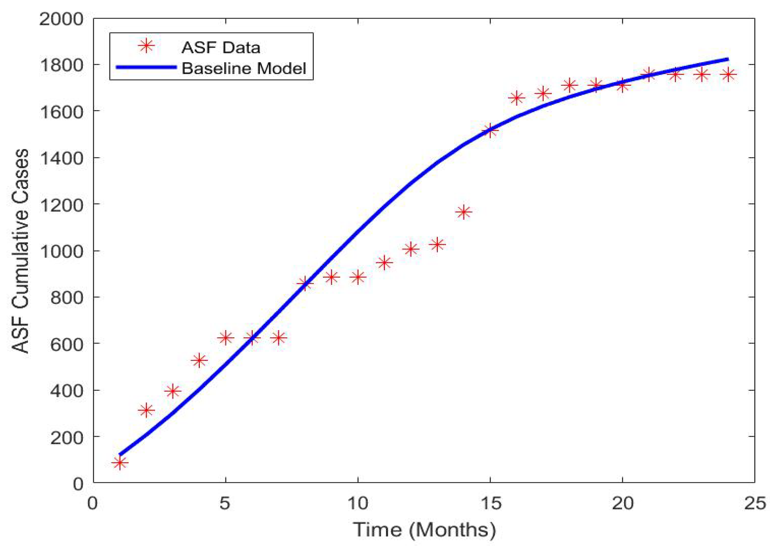
2.2. Model Fitting and Parameters Estimation

Validation of the newly African swine fever (ASF)-proposed epidemiological model is a crucial process to examine the disease’s transmission dynamics. For the presently formulated model, some parameters are available in the literature, while others are unknown. Some of the unknown parameters, $({\beta }_v,{\beta }_{ip},{\beta }_{is},{\beta }_{id},{\beta }_c,{\beta }_d,\alpha ,\omega ,{\delta }_{is}and{\delta }_{id})$, are estimated by fitting the ASF model to the monthly cumulative new cases of African swine fever (ASF) reported in Benin from January 2020 to December 2021. The nonlinear least-squares curve fitting algorithm, implemented in MATLAB (version R2021a) with the help of a routine “lsqcurvefit”function was used to perform the fitting and the estimation. The data are obtained from the National Directorate of Breeding’s Annual Reports of Benin.

3. Results

3.1. Analytical Results

3.1.1. Basic Properties

An important property of any mathematical model, including those describing biological processes, is its epidemiological and biological meaningfulness. Herein, we study the basic properties of the solutions of system (10), which are essential for proving stability results.

• Non-negativity and boundedness of the solution

Theorem 1.

System (10) is a dynamical system on the biologically feasible compact domain, as follows:

$$\begin{array}{c}\hfill \Gamma ={\Gamma }_1\times {\Gamma }_2\end{array}$$

(11)

where

$$\begin{array}{ccc}\hfill {\Gamma }_1& =& \{(S,I_p,I_s,I_d,C,R,D)\in {\mathbb{R}}_{+}^7:N=S+I_p+I_s+I_d+C+R,\hfill \\ & & 0\le N\le \frac{{\Lambda }_p}{{\mu }_p};D\le \frac{{\Lambda }_p}{{\mu }_p{\mu }_d}\left({\delta }_{is}+{\delta }_{id}\right)\},\hfill \end{array}$$

(12)

and

$$\begin{array}{c}\hfill {\Gamma }_2=\left\{V\in {\mathbb{R}}_{+},V\le \frac{A}{{\mu }_v-r}\right\},with,A=({\theta }_{ip}+{\theta }_{is}+{\theta }_{id}+{\theta }_C)\frac{{\Lambda }_p}{{\mu }_p}+\left({\delta }_{is}+{\delta }_{id}\right)\frac{{\Lambda }_p{\theta }_d}{{\mu }_p{\mu }_d}.\end{array}$$

(13)

Proof. 

The proof is provided in two steps.

Step 1: We show that the solutions $(S\left(t\right),I_p\left(t\right),I_s\left(t\right),I_d\left(t\right),C\left(t\right),R\left(t\right),D\left(t\right),V\left(t\right))$ of system (10) correspond to initial conditions, such that $S\left(0\right)>0$, $I_p\left(0\right)>0$, $I_s\left(0\right)>0$, $I_d\left(0\right)>0$, $C\left(0\right)>0$, $R\left(0\right)>0$, $D\left(0\right)>0$ and $V\left(0\right)>0$ are nonnegative.

To show that the solutions are positive, we show that the axes $S\left(t\right)=0$, $I_p\left(t\right)=0$, $I_s\left(t\right)=0$, $I_d\left(t\right)=0$, $C\left(t\right)=0$, $R\left(t\right)=0$, $D\left(t\right)=0$ and $V\left(t\right)=0$ are impassible barriers.

We prove that any trajectory that starts in ${\mathbb{R}}_{+}^8$ cannot leave ${\mathbb{R}}_{+}^8$.

Let $\tau$ = $sup\{t>0,S\left(t\right)>0,I_p\left(t\right)>0,I_s\left(t\right)>0,I_d\left(t\right)>0,C\left(t\right)>0,R\left(t\right)>0,D\left(t\right)>0,V\left(t\right)>0\}$.

The above initial conditions and the continuity of functions $S\left(t\right)$, $I_p\left(t\right)$, $I_s\left(t\right)$, $I_d\left(t\right)$, $C\left(t\right)$, $R\left(t\right)$, $D\left(t\right)$, and $V\left(t\right)$ ensure the existence of $\tau$.

If $\tau$ = $+\infty$, then all the solutions of the system of Equation (10) are positive.

Suppose $\tau$ < $+\infty$, then there is at least one solution, $S\left(t\right)$, $I_p\left(t\right)$, $I_s\left(t\right)$, $I_d\left(t\right)$, $C\left(t\right)$, $R\left(t\right)$, $D\left(t\right)$, and $V\left(t\right)$ which is equal to zero (from the definition of $\tau$ as a supremum).

Suppose that $S\left(\tau \right)=0$.

From the first equation of system (10), one has the following:

$$\dot{S}={\Lambda }_p-(\lambda +{\mu }_p)S.$$

(14)

Integrating Equation (14) from 0 to $\tau$ yields the following:

$$S\left(\tau \right)=e^{-{\int }_0^{\tau }(\lambda \left(u\right)+{\mu }_p)du}\left(S\left(0\right)+{\int }_0^{\tau }{\Lambda }_p.e^{{\int }_0^u(\lambda \left(v\right)+{\mu }_p)dv}du\right).$$

Hence, $S\left(\tau \right)>0$, which contradicts with $S\left(\tau \right)=0$, which we previously assumed. Thus, $S\left(t\right)>0$ for all $t>0$.

Similarly, positivity can be proved for the rest of the variables ($I_p$, $I_s$, $I_d$, C, R, and D) using this same approach except for the case where the virus lives freely in the environment (V).

Let us now prove the positivity of the last equation of system (10) for all $t>0$.

Using the positivity of $I_p$, $I_s$, $I_d$, C, and D, the last equation ($\dot{V}$) from system (10), can be written as follows:

$$\begin{array}{c}\hfill \begin{array}{ccc}\dot{V}\hfill & \ge \hfill & -\frac{1}{K_v}r{V}^2+(r-{\mu }_v)V.\hfill \end{array}\end{array}$$

(15)

Setting $z=V^{-1}$$\Rightarrow \dot{z}=-\dot{V}{V}^{-2}$, one has the following:

$$\begin{array}{ccc}\hfill \dot{V}+\frac{1}{K_v}r{V}^2-(r-{\mu }_v)V& \ge & 0,\hfill \\ \hfill \dot{V}{V}^{-2}-(r-{\mu }_v)V^{-1}+r{K}_v^{-1}& \ge & 0,\hfill \\ \hfill -\dot{z}-(r-{\mu }_v)z+r{K}_v^{-1}& \ge & 0.\hfill \end{array}$$

Then, following integration, we have the following:

$$\begin{array}{ccc}\hfill z\left(t\right)& =& e^{-{\int }_0^{\tau }(r-{\mu }_v)du}.\left(z\left(0\right)+{\int }_0^{\tau }r{K}_v^{-1}.e^{{\int }_0^u(r-{\mu }_v)dv}du\right).\hfill \end{array}$$

(16)

It clearly appears that $z\left(t\right)>0$ and since $z=V^{-1}$, hence $V\left(t\right)>0$, for all $t>0$.

Step 2: Now, we prove the boundedness of the trajectories of the model system (10).

Taking the total population of pigs at time t, we have the following:

$$\begin{array}{ccc}\hfill \frac{dN}{dt}& =& \frac{dS}{dt}+\frac{d{I}_p}{dt}+\frac{d{I}_s}{dt}+\frac{d{I}_d}{dt}+\frac{dC}{dt}+\frac{dR}{dt},\hfill \\ & =& {\Lambda }_p-{\mu }_{p}S-{\mu }_p{I}_p-{\mu }_p{I}_s-{\mu }_p{I}_d-{\mu }_{p}C-{\mu }_{p}R-{\delta }_{is}{I}_s-{\delta }_{id}{I}_d,\hfill \\ & =& {\Lambda }_p-{\mu }_p(S+I_p+I_s+I_d+C+R)-{\delta }_{is}{I}_s-{\delta }_{id}{I}_d,\hfill \\ \hfill \frac{dN}{dt}& =& {\Lambda }_p-{\mu }_{p}N-{\delta }_{is}{I}_s-{\delta }_{id}{I}_d,\hfill \end{array}$$

Using the fact that $(I_s,I_d)>0$, we have the following:

$$\begin{array}{ccc}\hfill \frac{dN}{dt}& \le & {\Lambda }_p-{\mu }_{p}N,\hfill \end{array}$$

Using Duhamel’s property, it follows that:

$$\begin{array}{ccc}\hfill N\left(t\right)& =& exp\left[{\int }_0^t-{\mu }_{p}d{t}^{\prime }\right].\left[N\left(0\right)+{\int }_0^{t}exp\left[-{\int }_0^{t^{\prime }}-{\mu }_{p}du\right].{\Lambda }_{p}dv\right],\hfill \\ & =& exp\left[-{\mu }_{p}t\right].\left[N\left(0\right)+{\Lambda }_p.{\int }_0^{t}exp\left[{\mu }_p{t}^{\prime }\right]dv\right],\hfill \\ & =& exp\left[-{\mu }_{p}t\right].{\left[N\left(0\right)+{\Lambda }_p.\left[\frac{1}{{\mu }_p}exp\left[{\mu }_p{t}^{\prime }\right]\right]\right]}_0^t,\hfill \\ & =& exp\left[-{\mu }_{p}t\right].\left[N\left(0\right)+\frac{{\Lambda }_p}{{\mu }_p}.exp\left[{\mu }_{p}t\right]-\frac{{\Lambda }_p}{{\mu }_p}\right],\hfill \\ \hfill N\left(t\right)& =& \frac{{\Lambda }_p}{{\mu }_p}+(N\left(0\right)-\frac{{\Lambda }_p}{{\mu }_p}).exp\left[-{\mu }_{p}t\right].\hfill \end{array}$$

Therefore, taking the limit when t tends to $+\infty$ gives the following:

$$\begin{array}{ccc}\hfill \underset{t\to +\infty }{lim}supN\left(t\right)& \le & \frac{{\Lambda }_p}{{\mu }_p}.\hfill \end{array}$$

It then follows that, as $t\to +\infty$, $N\left(t\right)\le \frac{{\Lambda }_p}{{\mu }_p}.$

Taking the death class equation ($\dot{D}$), we have the following:

$$\begin{array}{ccc}\hfill \frac{dD}{dt}& =& {\delta }_{is}{I}_s+{\delta }_{id}{I}_d-{\mu }_{d}D,\hfill \end{array}$$

But $N=S+I_p+I_s+I_d+C+R\le \frac{{\Lambda }_p}{{\mu }_p}$⇒$\left(I_s,I_d\right)\le \frac{{\Lambda }_p}{{\mu }_p}$, as $t\ge 0$.

It follows that

$$\begin{array}{ccc}\hfill \frac{dD}{dt}& \le & \frac{{\Lambda }_p}{{\mu }_p}\left({\delta }_{is}+{\delta }_{id}\right)-{\mu }_{d}D,\hfill \\ \hfill D\left(t\right)& \le & \frac{{\Lambda }_p}{{\mu }_p{\mu }_d}\left({\delta }_{is}+{\delta }_{id}\right)+(D\left(0\right)-\frac{{\Lambda }_p}{{\mu }_p}\left({\delta }_{is}+{\delta }_{id}\right)).exp\left[-{\mu }_{p}t\right].\hfill \end{array}$$

Therefore, taking the limit when t tends to $+\infty$ gives the following:

$$\begin{array}{ccc}\hfill \underset{t\to +\infty }{lim}supD\left(t\right)& \le & \frac{{\Lambda }_p}{{\mu }_p{\mu }_d}\left({\delta }_{is}+{\delta }_{id}\right).\hfill \end{array}$$

It then follows that as $t\to +\infty$, $D\left(t\right)\le \frac{{\Lambda }_p}{{\mu }_p{\mu }_d}\left({\delta }_{is}+{\delta }_{id}\right)$.

Now, taking the free-living virus equation and using the positivity of $V>0$ and the fact that $(I_p,I_s,I_d,C)\le \frac{{\Lambda }_p}{{\mu }_p}$ and $D\le \frac{{\Lambda }_p}{{\mu }_p{\mu }_d}\left({\delta }_{is}+{\delta }_{id}\right)$, one has the following inequality:

$$\begin{array}{ccc}\hfill \dot{V}& \le & A+(r-{\mu }_v)V,\hfill \end{array}$$

(17)

where $A=({\theta }_{ip}+{\theta }_{is}+{\theta }_{id}+{\theta }_C)\frac{{\Lambda }_p}{{\mu }_p}+\left({\delta }_{is}+{\delta }_{id}\right)\frac{{\Lambda }_p{\theta }_d}{{\mu }_p{\mu }_d}$.

Integrating (17) from zero to t yields the following:

$$\begin{array}{ccc}\hfill V\left(t\right)& \le & \frac{A}{{\mu }_v-r}+\left(V\left(0\right)-\frac{A}{{\mu }_v-r}\right).exp\left[(r-{\mu }_v)t\right].\hfill \end{array}$$

Taking the initial condition such that $V\left(0\right)>0$, and taking the limit of the above equation when t tends to $+\infty$ gives the following:

$$\underset{t\to +\infty }{lim}supV\left(t\right)\le \frac{A}{{\mu }_v-r}.$$

It then follows that as $t\to +\infty$, $V\left(t\right)\le \frac{A}{{\mu }_v-r}.$

Combining Step 1 and Step 2, Theorem 1 follows from the classical theory of dynamical systems. This concludes the proof. □

• Existence and uniqueness of a solution

The following theorem provides the result on the existence and uniqueness of the solution to system (10):

Theorem 2.

For any strictly positive initial condition, the solution of system (10) exists for all time $t\ge 0$ and is unique.

Proof. 

The right-hand side of system (10) is locally Lipschitzian and continuous. So, according to the Cauchy–Lipschitz theorem, one can deduce the existence and local uniqueness of the solution of system (10). The existence and the global uniqueness are deduced from the fact that the solutions are bounded. This achieves the proof. □

3.1.2. Disease-Free Equilibrium, Computation of the Control and Basic Reproduction Numbers

• Disease-free equilibrium

The disease-free equilibrium (DFE) state represents a condition where there is no infection or the infection can permanently be eradicated. At the equilibrium points, the rate of change of the model Equation (10) is assumed to be zero. To find the disease-free equilibrium point, we set the right-hand side of the model of Equation (10) to zero and evaluate it when the infective compartments are zero, i.e., at $I_p=0$, $I_s=0$, $I_d=0$, $C=0$, $D=0$, and $V=0$. In this case, from the system of Equation (10), we have the following:

$${\Lambda }_p-{\mu }_{p}S-\lambda S=0\Rightarrow S^0=\frac{{\Lambda }_P}{{\mu }_p}.$$

(18)

Hence, the disease-free equilibrium point is given by the following:

$$\begin{array}{c}\hfill E^0=(S^0,I_p^0,I_s^0,I_d^0,C^0,R^0,D^0,V^0)=\left(\frac{{\Lambda }_P}{{\mu }_p},0,0,0,0,0,0,0\right).\end{array}$$

(19)

• Computation of the Control Reproduction Number, ${\mathcal{R}}_c$

To assess whether the implemented control measures, such as early detection and isolation of infectious cases and proper disposal of ASFV-infected pig cadavers via burial or cremation, are effective in controlling African swine fever (ASF) outbreaks, we computed the control reproduction number, ${\mathcal{R}}_c$. The control reproduction number, ${\mathcal{R}}_c$, is defined in mathematical epidemiology as the expected average number of secondary infections caused by one infectious animal (pig) in a fully susceptible population throughout its infectious period. To compute the control reproduction number, we used the next-generation matrix method formulated in [28] and as reported in [29], which is given by $\tau \left(F{W}^{-1}\right)$, where $\tau$ denotes the spectral radius, F denotes the new infection terms, and W denotes the remaining transition terms.

The vectors representing the production of new infections and the transition parts are, respectively, as follows:

$$\begin{array}{c}\hfill \mathcal{F}\left(x\right)=\left(\begin{array}{c}\frac{{\beta }_{ip}{I}_{p}S+{\beta }_{is}{I}_{s}S+{\beta }_{id}{I}_{d}S+{\beta }_{c}CS+{\beta }_{d}DS}{N}+\frac{{\beta }_{v}VS}{K+V}\\ 0\\ 0\\ 0\\ 0\\ 0\end{array}\right),\end{array}$$

and

$$\begin{array}{c}\hfill \mathcal{W}\left(x\right)=\left(\begin{array}{c}(\alpha +{\tau }_{ip}+{\mu }_p)I_p\\ -\rho \alpha I_p-\omega C+({\delta }_{is}+{\gamma }_{is}+{\tau }_{is}+{\mu }_p)I_s\\ -{\tau }_{is}{I}_s-{\tau }_{ip}{I}_p-{\tau }_{c}C+({\gamma }_{id}+{\delta }_{id}+{\mu }_p)I_d\\ -(1-\rho )\alpha I_p+(\omega +{\tau }_c+{\gamma }_c+{\mu }_p)C\\ -{\delta }_{is}{I}_s-{\delta }_{id}{I}_d+{\mu }_{d}D\\ -rV\left(1-\frac{V}{K_v}\right)+{\mu }_{v}V-{\theta }_{ip}{I}_p-{\theta }_{is}{I}_s-{\theta }_{id}{I}_d-{\theta }_{c}C-{\theta }_{d}D\end{array}\right).\end{array}$$

where $x={(I_p,I_s,I_d,C,D,V)}^T$.

The Jacobian matrices of $\mathcal{F}\left(x\right)$ and $\mathcal{W}\left(x\right)$ around the disease-free equilibrium $E^0$ are as follows:

$$\begin{array}{c}\hfill F=\left(\begin{array}{cccccc}{\beta }_{ip}& {\beta }_{is}& {\beta }_{id}& {\beta }_c& {\beta }_d& \frac{{\Lambda }_p{\beta }_v}{K{\mu }_p}\\ 0& 0& 0& 0& 0& 0\\ 0& 0& 0& 0& 0& 0\\ 0& 0& 0& 0& 0& 0\\ 0& 0& 0& 0& 0& 0\\ 0& 0& 0& 0& 0& 0\end{array}\right)\end{array}$$

and

$$\begin{array}{c}\hfill W=\left(\begin{array}{cccccc}\alpha +{\tau }_{ip}+{\mu }_p& 0& 0& 0& 0& 0\\ -\rho \alpha & {\delta }_{is}+{\gamma }_{is}+{\tau }_{is}+{\mu }_p& 0& -\omega & 0& 0\\ -{\tau }_{ip}& -{\tau }_{is}& {\gamma }_{id}+{\delta }_{id}+{\mu }_p& -{\tau }_c& 0& 0\\ -(1-\rho )\alpha & 0& 0& \omega +{\tau }_c+{\gamma }_c+{\mu }_p& 0& 0\\ 0& -{\delta }_{is}& -{\delta }_{id}& 0& {\mu }_d& 0\\ -{\theta }_{ip}& -{\theta }_{is}& -{\theta }_{id}& -{\theta }_c& -{\theta }_d& {\mu }_v-r\end{array}\right)\end{array}$$

Thus, from system (10), the control reproduction number is given as follows: ${\mathcal{R}}_c={\mathcal{R}}_c^{I_p}+{\mathcal{R}}_c^C+{\mathcal{R}}_c^{I_s}+{\mathcal{R}}_c^{I_d}+{\mathcal{R}}_c^D+{\mathcal{R}}_c^V$, which is the sum of the average numbers of animals (pigs) infected by introducing, respectively, a single ASFV presymptomatic, carrier animal (pig), symptomatic, detected, dead animal (pig), and a single load of the virus in a susceptible unit, where

$$\begin{array}{c}\hfill \begin{array}{ccc}{\mathcal{R}}_c^{I_p}\hfill & =\hfill & \frac{{\beta }_{ip}}{\left(\alpha +{\tau }_{ip}+{\mu }_p\right)},\hfill \\ {\mathcal{R}}_c^C\hfill & =\hfill & \frac{1}{\left(\alpha +{\tau }_{ip}+{\mu }_p\right)}\left[{\displaystyle \frac{\left(1-\rho \right)\alpha {\beta }_c}{\left(\omega +{\tau }_c+{\gamma }_c+{\mu }_p\right)}}\right],\hfill \\ {\mathcal{R}}_c^{I_s}\hfill & =\hfill & \frac{1}{\left(\alpha +{\tau }_{ip}+{\mu }_p\right)}\left[{\displaystyle \frac{\alpha {\beta }_{is}{B}_1}{\left({\delta }_{is}+{\gamma }_{is}+{\tau }_{is}+{\mu }_p\right)\left(\omega +{\tau }_c+{\gamma }_c+{\mu }_p\right)}}\right],\hfill \\ {\mathcal{R}}_c^{I_d}\hfill & =\hfill & \frac{1}{\left(\alpha +{\tau }_{ip}+{\mu }_p\right)}\left[{\displaystyle \frac{{\beta }_{id}\left[\left(\omega +{\tau }_c+{\gamma }_c+{\mu }_p\right)B_2+\left(1-\rho \right)\alpha B_3)\right]}{\left({\delta }_{is}+{\gamma }_{is}+{\tau }_{is}+{\mu }_p\right)\left({\gamma }_{id}+{\delta }_{id}+{\mu }_p\right)\left(\omega +{\tau }_c+{\gamma }_c+{\mu }_p\right)}}\right],\hfill \\ {\mathcal{R}}_c^D\hfill & =\hfill & \frac{1}{\left(\alpha +{\tau }_{ip}+{\mu }_p\right)}\left[{\displaystyle \frac{{\beta }_d\left[\left(\alpha B_1{C}_1\right)+{\delta }_{id}\left({\delta }_{is}+{\gamma }_{is}+{\tau }_{is}+{\mu }_p\right)C_2\right]}{{\mu }_d\left({\delta }_{is}+{\gamma }_{is}+{\tau }_{is}+{\mu }_p\right)\left({\gamma }_{id}+{\delta }_{id}+{\mu }_p\right)\left(\omega +{\tau }_c+{\gamma }_c+{\mu }_p\right)}}\right],\hfill \\ {\mathcal{R}}_c^V\hfill & =\hfill & \frac{1}{\left(\alpha +{\tau }_{ip}+{\mu }_p\right)}\left[{\displaystyle \frac{{\Lambda }_p{\beta }_v\left[\left(B_2{C}_3\right)+\left(B_3{C}_4\right)+\left(\alpha B_1{C}_5\right)+\left({\delta }_{is}+{\gamma }_{is}+{\tau }_{is}+{\mu }_p\right)\left({\gamma }_{id}+{\delta }_{id}+{\mu }_p\right){\mu }_d{C}_6\right]}{K{\mu }_p{\mu }_d\left({\delta }_{is}+{\gamma }_{is}+{\tau }_{is}+{\mu }_p\right)\left({\gamma }_{id}+{\delta }_{id}+{\mu }_p\right)\left(\omega +{\tau }_c+{\gamma }_c+{\mu }_p\right)\left({\mu }_v-r\right)}}\right]\hfill \end{array}\end{array}$$

with

$$\begin{array}{c}\hfill \begin{array}{cc}{B}_1=\left[\left(\omega +{\tau }_c+{\gamma }_c+{\mu }_p\right)\rho +(1-\rho )\omega \right],\hfill & B_2=\left[\rho \alpha {\tau }_{is}+\left({\delta }_{is}+{\gamma }_{is}+{\tau }_{is}+{\mu }_p\right){\tau }_{ip}\right],\hfill \\ B_3=\left[\omega {\tau }_{is}+\left({\delta }_{is}+{\gamma }_{is}+{\tau }_{is}+{\mu }_p\right){\tau }_c\right],\hfill & C_1=\left[{\tau }_{is}{\delta }_{id}+\left({\gamma }_{id}+{\delta }_{id}+{\mu }_p\right){\delta }_{is}\right],\hfill \\ C_2=\left[\left(\omega +{\tau }_c+{\gamma }_c+{\mu }_p\right){\tau }_{ip}+(1-\rho )\alpha {\tau }_c\right],\hfill & C_3=\left(\omega +{\tau }_c+{\gamma }_c+{\mu }_p\right)\left[{\mu }_d{\theta }_{id}+{\delta }_{id}{\theta }_d\right],\hfill \\ C_4=(1-\rho )\alpha \left[{\mu }_d{\theta }_{id}+{\delta }_{id}{\theta }_d\right],\hfill & C_5=\left({\gamma }_{id}+{\delta }_{id}+{\mu }_p\right)\left[{\delta }_{is}{\theta }_d+{\mu }_d{\theta }_{is}\right],\hfill \\ C_6=\left[\left(\omega +{\tau }_c+{\gamma }_c+{\mu }_p\right){\theta }_{ip}+(1-\rho )\alpha {\theta }_c\right].\hfill \end{array}\end{array}$$

• Computation of the basic reproduction number, ${\mathcal{R}}_0$

In the absence of early detection and isolation of infectious cases, as well as proper disposal of ASFV-infected pigs’ cadavers via burial or cremation, the control reproduction number reduces to the basic reproduction number, denoted by ${\mathcal{R}}_0$, which is given by the following:

$$\begin{array}{c}\hfill {\mathcal{R}}_0={\mathcal{R}}_c|{\tau }_{ip}={\tau }_{is}={\tau }_c={\mu }_d=0.\end{array}$$

Then, we have the following:

$$\begin{array}{c}\hfill {\mathcal{R}}_0={\mathcal{R}}_0^{I_p}+{\mathcal{R}}_0^C+{\mathcal{R}}_0^{I_s}+{\mathcal{R}}_0^{I_d}+{\mathcal{R}}_0^D+{\mathcal{R}}_0^V\end{array}$$

where

$$\begin{array}{c}\hfill \begin{array}{ccc}{\mathcal{R}}_0^{I_p}\hfill & =\hfill & \frac{{\beta }_{ip}}{\left(\alpha +{\mu }_p\right)},\hfill \\ {\mathcal{R}}_0^C\hfill & =\hfill & \frac{1}{\left(\alpha +{\mu }_p\right)}\left[{\displaystyle \frac{\left(1-\rho \right)\alpha {\beta }_c}{\left(\omega +{\gamma }_c+{\mu }_p\right)}}\right],\hfill \\ {\mathcal{R}}_0^{I_s}\hfill & =\hfill & \frac{1}{\left(\alpha +{\mu }_p\right)}\left[{\displaystyle \frac{\alpha {\beta }_{is}{B}_1^{\prime }}{\left({\delta }_{is}+{\gamma }_{is}+{\mu }_p\right)\left(\omega +{\gamma }_c+{\mu }_p\right)}}\right],\hfill \\ {\mathcal{R}}_0^{I_d}\hfill & =\hfill & \frac{1}{\left(\alpha +{\mu }_p\right)}\left[{\displaystyle \frac{{\beta }_{id}\left[\left(\omega +{\gamma }_c+{\mu }_p\right)B_2^{\prime }+\left(1-\rho \right)\alpha B_3^{\prime })\right]}{\left({\delta }_{is}+{\gamma }_{is}+{\mu }_p\right)\left({\gamma }_{id}+{\delta }_{id}+{\mu }_p\right)\left(\omega +{\gamma }_c+{\mu }_p\right)}}\right],\hfill \\ {\mathcal{R}}_0^D\hfill & =\hfill & \frac{1}{\left(\alpha +{\mu }_p\right)}\left[{\displaystyle \frac{{\beta }_d\left[\left(\alpha B_1^{\prime }{C}_1^{\prime }\right)+{\delta }_{id}\left({\delta }_{is}+{\gamma }_{is}+{\mu }_p\right)C_2^{\prime }\right]}{\left({\delta }_{is}+{\gamma }_{is}+{\mu }_p\right)\left({\gamma }_{id}+{\delta }_{id}+{\mu }_p\right)\left(\omega +{\gamma }_c+{\mu }_p\right)}}\right],\hfill \\ {\mathcal{R}}_0^V\hfill & =\hfill & \frac{1}{\left(\alpha +{\mu }_p\right)}\left[{\displaystyle \frac{{\Lambda }_p{\beta }_v\left[\left(B_2^{\prime }{C}_3^{\prime }\right)+\left(B_3^{\prime }{C}_4^{\prime }\right)+\left(\alpha B_1^{\prime }{C}_5^{\prime }\right)+\left({\delta }_{is}+{\gamma }_{is}+{\mu }_p\right)\left({\gamma }_{id}+{\delta }_{id}+{\mu }_p\right)C_6^{\prime }\right]}{K{\mu }_p\left({\delta }_{is}+{\gamma }_{is}+{\mu }_p\right)\left({\gamma }_{id}+{\delta }_{id}+{\mu }_p\right)\left(\omega +{\gamma }_c+{\mu }_p\right)\left({\mu }_v-r\right)}}\right],\hfill \end{array}\end{array}$$

with

$$\begin{array}{c}\hfill \begin{array}{cc}{B}_1^{\prime }=\left[\left(\omega +{\gamma }_c+{\mu }_p\right)\rho +(1-\rho )\omega \right],\hfill & B_2^{\prime }=\left[\rho \alpha +\left({\delta }_{is}+{\gamma }_{is}+{\mu }_p\right)\right],\hfill \\ B_3^{\prime }=\left[\omega +\left({\delta }_{is}+{\gamma }_{is}+{\mu }_p\right)\right],\hfill & C_1^{\prime }=\left[{\delta }_{id}+\left({\gamma }_{id}+{\delta }_{id}+{\mu }_p\right){\delta }_{is}\right],\hfill \\ C_2^{\prime }=\left[\left(\omega +{\gamma }_c+{\mu }_p\right)+(1-\rho )\alpha \right],\hfill & C_3^{\prime }=\left(\omega +{\gamma }_c+{\mu }_p\right)\left[{\theta }_{id}+{\delta }_{id}{\theta }_d\right],\hfill \\ C_4^{\prime }=(1-\rho )\alpha \left[{\theta }_{id}+{\delta }_{id}{\theta }_d\right],\hfill & C_5^{\prime }=\left({\gamma }_{id}+{\delta }_{id}+{\mu }_p\right)\left[{\delta }_{is}{\theta }_d+{\theta }_{is}\right],\hfill \\ C_6^{\prime }=\left[\left(\omega +{\gamma }_c+{\mu }_p\right){\theta }_{ip}+(1-\rho )\alpha {\theta }_c\right].\hfill \end{array}\end{array}$$

3.1.3. Local and Global Stabilities of the Disease-Free Equilibrium

• Local stability of the disease-free equilibrium

Using Theorem A1 given in Appendix A and in [28], the following result is straightforward.

Lemma 1.

The disease-free equilibrium $E^0$ of system (10) is locally asymptotically stable, if ${\mathcal{R}}_c\le 1$, and unstable if ${\mathcal{R}}_c>1$ in Γ.

Biologically speaking Lemma 1 implies that:

• If ${\mathcal{R}}_c\le 1$, then each infected animal (pig) generates, on average, less than one new infected animal (pig) during his period of infectiousness. In this case, we can expect the disease to disappear in the community.
• If ${\mathcal{R}}_c>1$, then each infected animal (pig) generates, on average, more than one new infected animal. In this case, the disease could persist in the community.

For better control of the disease, it is important to widen the basin of attraction of the disease-free equilibrium. For this reason, we will study the overall stability of the disease-free equilibrium.

• Global stability of the disease-free equilibrium

Here, we explore the global asymptotic stability of the disease-free equilibrium of the model (Figure 1). For that, one common approach is to construct an appropriate Lyapunov function [30] or use Kamgang and Sallet’s theorem [31]. We have found, however, that it is simpler to apply the following two outstanding theories, namely, the comparison theory for monotone dynamical systems introduced by [32,33] and the theory of asymptotically autonomous systems introduced by [34], to prove the global attractivity of the disease-free equilibrium. The following theorem gives the global asymptotic stability for the DFE:

Theorem 3.

If ${\mathcal{R}}_c\le 1$, the disease-free equilibrium is globally asymptotically stable.

Proof. 

Considering the $(I_p,I_s,I_d,C,D,V)$ sub-equations in system (10), and using the fact that $S\left(t\right)\le \frac{{\Lambda }_P}{{\mu }_P}$ for all $t\ge 0$, one has the following comparison linear system in (${\overline{I}}_p,{\overline{I}}_s,{\overline{I}}_d,\overline{C},\overline{D},\overline{V}$):

$$\begin{array}{c}\hfill \left\{\begin{array}{c}{\dot{\overline{I}}}_p=\left[\frac{{\beta }_{ip}{\overline{I}}_p+{\beta }_{is}{\overline{I}}_s+{\beta }_{id}{\overline{I}}_d+{\beta }_c\overline{C}+{\beta }_d\overline{D}}{\overline{N}}\right]\frac{{\Lambda }_p}{{\mu }_p}+\frac{{\Lambda }_p{\beta }_v}{K{\mu }_p}\overline{V}-(\alpha +{\tau }_{ip}+{\mu }_p){\overline{I}}_p,\hfill \\ {\dot{\overline{I}}}_s=\rho \alpha {\overline{I}}_p+\omega \overline{C}-({\delta }_{is}+{\gamma }_{is}+{\tau }_{is}+{\mu }_p){\overline{I}}_s,\hfill \\ {\dot{\overline{I}}}_d={\tau }_{is}{\overline{I}}_s+{\tau }_{ip}{\overline{I}}_p+{\tau }_c\overline{C}-({\gamma }_{id}+{\delta }_{id}+{\mu }_p){\overline{I}}_d,\hfill \\ \dot{\overline{C}}=(1-\rho )\alpha {\overline{I}}_p-(\omega +{\tau }_c+{\gamma }_c+{\mu }_p)\overline{C},\hfill \\ \dot{\overline{D}}={\delta }_{is}{\overline{I}}_s+{\delta }_{id}{\overline{I}}_d-{\mu }_d\overline{D},\hfill \\ \dot{\overline{V}}=\left(r-{\mu }_v\right)\overline{V}+{\theta }_{ip}{\overline{I}}_p+{\theta }_{is}{\overline{I}}_s+{\theta }_{id}{\overline{I}}_d+{\theta }_c\overline{C}+{\theta }_d\overline{D}.\hfill \end{array}\right.\end{array}$$

(20)

Note that $(0,0,0,0,0,0)$ is the unique equilibrium of the linear system (20). The linear system of Equation (20) can be written in the following compact form:

$$\begin{array}{c}\hfill \dot{X}=(\hat{F}-W)X.\end{array}$$

(21)

where $X={({\overline{I}}_p,{\overline{I}}_s,{\overline{I}}_d,\overline{C},\overline{D},\overline{V})}^T$,

$$\begin{array}{c}\hfill W=\left(\begin{array}{cccccc}\alpha +{\tau }_{ip}+{\mu }_p& 0& 0& 0& 0& 0\\ -\rho \alpha & {\delta }_{is}+{\gamma }_{is}+{\tau }_{is}+{\mu }_p& 0& -\omega & 0& 0\\ -{\tau }_{ip}& -{\tau }_{is}& {\gamma }_{id}+{\delta }_{id}+{\mu }_p& -{\tau }_c& 0& 0\\ -(1-\rho )\alpha & 0& 0& \omega +{\tau }_c+{\gamma }_c+{\mu }_p& 0& 0\\ 0& -{\delta }_{is}& -{\delta }_{id}& 0& {\mu }_d& 0\\ -{\theta }_{ip}& -{\theta }_{is}& -{\theta }_{id}& -{\theta }_c& -{\theta }_d& {\mu }_v-r\end{array}\right),\end{array}$$

$$\begin{array}{ccc}\hfill and,& \hfill & \hfill \hat{F}=\left(\begin{array}{cccccc}{\beta }_{ip}& {\beta }_{is}& {\beta }_{id}& {\beta }_c& {\beta }_d& \frac{{\Lambda }_p{\beta }_v}{K{\mu }_p}\\ 0& 0& 0& 0& 0& 0\\ 0& 0& 0& 0& 0& 0\\ 0& 0& 0& 0& 0& 0\\ 0& 0& 0& 0& 0& 0\\ 0& 0& 0& 0& 0& 0\end{array}\right).\end{array}$$

Then, Equation (21) can be rewritten as follows:

$$\begin{array}{ccc}\hfill \frac{d}{dt}\left(\begin{array}{c}{\overline{I}}_p\left(t\right)\\ {\overline{I}}_s\left(t\right)\\ {\overline{I}}_d\left(t\right)\\ \overline{C}\left(t\right)\\ \overline{D}\left(t\right)\\ \overline{V}\left(t\right)\end{array}\right)& =& (\hat{F}-W)\left(\begin{array}{c}{\overline{I}}_p\left(t\right)\\ {\overline{I}}_s\left(t\right)\\ {\overline{I}}_d\left(t\right)\\ \overline{C}\left(t\right)\\ \overline{D}\left(t\right)\\ \overline{V}\left(t\right)\end{array}\right)\Rightarrow \dot{X}=(\hat{F}-W)X\hfill \end{array}$$

(22)

with

$$\begin{array}{c}\hfill (\hat{F}-W)=\left(\begin{array}{cccccc}{\beta }_{ip}-(\alpha +{\tau }_{ip}+{\mu }_p)& {\beta }_{is}& {\beta }_{id}& {\beta }_c& {\beta }_d& \frac{{\Lambda }_p{\beta }_v}{K{\mu }_p}\\ \rho \alpha & -({\delta }_{is}+{\gamma }_{is}+{\tau }_{is}+{\mu }_p)& 0& \omega & 0& 0\\ {\tau }_{ip}& {\tau }_{is}& -({\gamma }_{id}+{\delta }_{id}+{\mu }_p)& {\tau }_c& 0& 0\\ (1-\rho )\alpha & 0& 0& -(\omega +{\tau }_c+{\gamma }_c+{\mu }_p)& 0& 0\\ 0& {\delta }_{is}& {\delta }_{id}& 0& -{\mu }_d& 0\\ {\theta }_{ip}& {\theta }_{is}& {\theta }_{id}& {\theta }_c& {\theta }_d& r-{\mu }_v\end{array}\right).\end{array}$$

(23)

Note that the solution $X=(0,0,0,0,0,0)$ is the unique equilibrium of the linear comparison system (21), which is globally asymptotically stable if and only if $\tau \left(\hat{F}{W}^{-1}\right)<1$.

Obviously, ${\mathcal{R}}_c$ is derived from $\tau \left(\hat{F}{W}^{-1}\right)$, as given above.

Therefore, it follows that all solutions of the linear comparison system (21) converge to the trivial solution $X=(0,0,0,0,0,0)$ when $t\to \infty$, with $t>T$. Moreover, one can see that ($\hat{F}-W$) is a Metzler matrix (M-matrix) (the off-diagonal elements are nonnegative) and irreducible. Thus, by the comparison theorem for monotone dynamical systems [32,33], one can conclude that the $I_p$, $I_s$, $I_d$, C, D, and V components of system (10) also converge to zero when $t\to \infty$, with $t>T$.

Now, substituting $I_p=I_s=I_d=C=D=V=0,$ into the differential equations for the rate of change of the $S\left(t\right)$ and $R\left(t\right)$ compartments of the model (10) gives the following asymptotic (limiting) autonomous linear system:

$$\begin{array}{c}\hfill \left\{\begin{array}{c}\dot{S}\le {\Lambda }_p-{\mu }_{p}S\hfill \\ \dot{R}\le -{\mu }_{p}R.\hfill \end{array}\right.\end{array}$$

(24)

Therefore, we can conclude the following:

$$R\left(t\right)\to 0;\mathrm{and}S\left(t\right)\to \frac{{\Lambda }_P}{{\mu }_P},ast\to \infty .$$

(25)

Then, using the comparison theorem, one can conclude that $S\left(t\right)$ converges to $S0$ and that $R\left(t\right)$ converges to $R0$. Thus, the equilibrium point ($S^0,R^0$) of system (10) is globally asymptotically stable in $\Gamma$. Following the theory of asymptotically autonomous systems [34], one can conclude that the disease-free equilibrium (DFE) $\left(E^0\right)$ is attractive in $\Gamma$. Since the local stability has been proven, the DFE $\left(E^0\right)$ is globally asymptotically stable in $\Gamma$. This concludes the proof. □

3.1.4. The Endemic Equilibrium Point and Its Stability

Herein, we study the existence and stability of the endemic equilibrium of the model (Figure 1). Let $E^{★}=(S^{*},I_p^{*},I_s^{*},I_d^{*},C^{*},R^{*},D^{*},V^{*})$ be the endemic equilibrium of system (10) with $S^{*}\ne 0,I_p^{*}\ne 0,I_s^{*}\ne 0,I_d^{*}\ne 0,C^{*}\ne 0,R^{*}\ne 0,D^{*}\ne 0,and{V}^{*}\ne 0$ satisfying the following system:

$$\begin{array}{c}\hfill \left\{\begin{array}{c}{\Lambda }_p-({\lambda }^{*}+{\mu }_p)S^{*}=0,\hfill \\ {\lambda }^{*}{S}^{*}-(\alpha +{\tau }_{ip}+{\mu }_p)I_p^{*}=0,\hfill \\ \rho \alpha I_p^{*}+\omega C^{*}-({\delta }_{is}+{\gamma }_{is}+{\tau }_{is}+{\mu }_p)I_s^{*}=0,\hfill \\ {\tau }_{is}{I}_s^{*}+{\tau }_{ip}{I}_p^{*}+{\tau }_c{C}^{*}-({\gamma }_{id}+{\delta }_{id}+{\mu }_p)I_d^{*}=0,\hfill \\ (1-\rho )\alpha I_p^{*}-(\omega +{\tau }_c+{\gamma }_c+{\mu }_p)C^{*}=0,\hfill \\ {\gamma }_{is}{I}_s^{*}+{\gamma }_{id}{I}_d^{*}+{\gamma }_c{C}^{*}-{\mu }_p{R}^{*}=0,\hfill \\ {\delta }_{is}{I}_s^{*}+{\delta }_{id}{I}_d^{*}-{\mu }_d{D}^{*}=0,\hfill \\ r{V}^{*}\left(1-\frac{V^{*}}{K_v}\right)-{\mu }_v{V}^{*}+{\theta }_{ip}{I}_p^{*}+{\theta }_{is}{I}_s^{*}+{\theta }_{id}{I}_d^{*}+{\theta }_c{C}^{*}+{\theta }_d{D}^{*}=0,\hfill \end{array}\right.\end{array}$$

(26)

where

$${\lambda }^{*}=\frac{{\beta }_{ip}{I}_p^{*}+{\beta }_{is}{I}_s^{*}+{\beta }_{id}{I}_d^{*}+{\beta }_c{C}^{*}+{\beta }_d{D}^{*}}{N^{*}}+{\beta }_v\frac{V^{*}}{K+V^{*}}.$$

(27)

is the force of infection at the steady state.

From the first equation of system (26), one has the following:

$$\begin{array}{ccc}\hfill S^{★}& =& \frac{{\Lambda }_p}{({\mu }_p+{\lambda }^{★})}.\hfill \end{array}$$

(28)

Plugging Equation (28) into the second equation of system (26), one has the following:

$$\begin{array}{ccc}\hfill I_p^{★}& =& \frac{{\lambda }^{★}{\Lambda }_p}{(\alpha +{\tau }_{ip}+{\mu }_p)({\mu }_p+{\lambda }^{★})}.\hfill \end{array}$$

(29)

Putting the expressions in Equations (28) and (29) into the fifth equation of system (26) yields the following:

$$\begin{array}{ccc}\hfill C^{★}& =& \frac{(1-\rho )\alpha {\lambda }^{★}{\Lambda }_p}{\left(\omega +{\tau }_c+{\gamma }_c+{\mu }_p\right)\left(\alpha +{\tau }_{ip}+{\mu }_p\right)({\mu }_p+{\lambda }^{★})}.\hfill \end{array}$$

(30)

Plugging Equations (29) and (30) into the third equation of system (26) yields the following:

$$\begin{array}{ccc}\hfill I_s^{★}& =& \frac{\alpha {\lambda }^{★}{\Lambda }_p{B}_1}{\left(\omega +{\tau }_c+{\gamma }_c+{\mu }_p\right)\left({\delta }_{is}+{\gamma }_{is}+{\tau }_{is}+{\mu }_p\right)\left(\alpha +{\tau }_{ip}+{\mu }_p\right)({\mu }_p+{\lambda }^{★})},\hfill \end{array}$$

(31)

where

$$\begin{array}{ccc}\hfill B_1& =& \left[\left(\omega +{\tau }_c+{\gamma }_c+{\mu }_p\right)\rho +(1-\rho )\omega \right].\hfill \end{array}$$

Combining Equations (29)–(31) into the fourth equation of system (26) gives the following:

$$\begin{array}{ccc}\hfill I_d^{★}& =& \frac{{\lambda }^{★}{\Lambda }_p\left[\left(\omega +{\tau }_c+{\gamma }_c+{\mu }_p\right)B_2+(1-\rho )\alpha B_3\right]}{B_4\left(\omega +{\tau }_c+{\gamma }_c+{\mu }_p\right)\left(\alpha +{\tau }_{ip}+{\mu }_p\right)({\mu }_p+{\lambda }^{★})},\hfill \end{array}$$

(32)

where

$$\begin{array}{c}\hfill \begin{array}{cc}{B}_2=\left[\rho \alpha {\tau }_{is}+\left({\delta }_{is}+{\gamma }_{is}+{\tau }_{is}+{\mu }_p\right){\tau }_{ip}\right],\hfill & B_3=\left[\omega {\tau }_{is}+\left({\delta }_{is}+{\gamma }_{is}+{\tau }_{is}+{\mu }_p\right){\tau }_c\right],\mathrm{and}\hfill \\ B_4=\left({\gamma }_{id}+{\delta }_{id}+{\mu }_p\right)\left({\delta }_{is}+{\gamma }_{is}+{\tau }_{is}+{\mu }_p\right).\hfill \end{array}\end{array}$$

Plugging Equations (30)–(32) into the sixth equation of system (26) yields the following:

$$\begin{array}{ccc}\hfill R^{★}& =& \frac{{\lambda }^{★}{\Lambda }_p\left[{\gamma }_{is}\left({\gamma }_{id}+{\delta }_{id}+{\mu }_p\right)\alpha B_1+{\gamma }_{id}\left(\omega +{\tau }_c+{\gamma }_c+{\mu }_p\right)B_2+(1-\rho )\alpha \left({\gamma }_{id}{B}_3+{\gamma }_c{B}_4\right)\right]}{{\mu }_p{B}_4\left(\omega +{\tau }_c+{\gamma }_c+{\mu }_p\right)\left(\alpha +{\tau }_{ip}+{\mu }_p\right)({\mu }_p+{\lambda }^{★})}\hfill \end{array}$$

(33)

Putting the expressions in Equations (31) and (32) into the seventh equation of system (26) yields the following:

$$\begin{array}{ccc}\hfill D^{★}& =& \frac{{\lambda }^{★}{\Lambda }_p\left[\left({\gamma }_{id}+{\delta }_{id}+{\mu }_p\right)\alpha {\delta }_{is}{B}_1+\left(\omega +{\tau }_c+{\gamma }_c+{\mu }_p\right){\delta }_{id}{B}_2+(1-\rho )\alpha {\delta }_{id}{B}_3\right]}{{\mu }_d{B}_4\left(\omega +{\tau }_c+{\gamma }_c+{\mu }_p\right)\left(\alpha +{\tau }_{ip}+{\mu }_p\right)({\mu }_p+{\lambda }^{★})},\hfill \end{array}$$

(34)

with all this in mind, from the Equation (27) one has that:

$$\begin{array}{ccc}\hfill V^{★}& =& \frac{\left({\beta }_{ip}{I}_p^{*}+{\beta }_{is}{I}_s^{*}+{\beta }_{id}{I}_d^{*}+{\beta }_c{C}^{*}+{\beta }_d{D}^{*}\right)K-{\lambda }^{★}{N}^{*}K}{\left[{\lambda }^{★}{N}^{*}-{\beta }_v{N}^{*}-\left({\beta }_{ip}{I}_p^{*}+{\beta }_{is}{I}_s^{*}+{\beta }_{id}{I}_d^{*}+{\beta }_c{C}^{*}+{\beta }_d{D}^{*}\right)\right]}.\hfill \end{array}$$

Note that at steady state, the size of the total population of pigs satisfies the following equation:

$$\begin{array}{ccc}\hfill {\Lambda }_p-{\mu }_p{N}^{★}-({\delta }_{is}{I}_s+{\delta }_{id}{I}_d)=0& \Rightarrow & N^{★}=\frac{{\Lambda }_p-({\delta }_{is}{I}_s+{\delta }_{id}{I}_d)}{{\mu }_p}.\hfill \end{array}$$

Then,

$$\begin{array}{c}\hfill N^{★}=\frac{{\Lambda }_p{B}_6\left({\mu }_p+\lambda \right)-{\lambda }^{★}{\Lambda }_p{B}_5}{{\mu }_p{B}_6\left({\mu }_p+\lambda \right)},\end{array}$$

(35)

where

$$\begin{array}{cc}\hfill B_5=\left[\alpha {\delta }_{is}{B}_1+\frac{\left(\omega +{\tau }_c+{\gamma }_c+{\mu }_p\right){\delta }_{id}{B}_2}{\left({\gamma }_{id}+{\delta }_{id}+{\mu }_p\right)}+\frac{(1-\rho )\alpha {\delta }_{id}{B}_3}{\left({\gamma }_{id}+{\delta }_{id}+{\mu }_p\right)}\right],& \mathrm{and}\\ \hfill B_6=\left(\omega +{\tau }_c+{\gamma }_c+{\mu }_p\right)\left({\delta }_{is}+{\gamma }_{is}+{\tau }_{is}+{\mu }_p\right)\left(\alpha +{\tau }_{ip}+{\mu }_p\right).\end{array}$$

Then, it follows that

$$\begin{array}{ccc}\hfill V^{★}& =& \frac{{\lambda }^{★}{\Lambda }_{p}K{D}_1{D}_2-{\lambda }^{★}K\left[{\Lambda }_p{B}_6({\mu }_p+{\lambda }^{★})-{\lambda }^{★}{\Lambda }_p{B}_5\right]}{\left[{\Lambda }_p{B}_6({\mu }_p+{\lambda }^{★})-{\lambda }^{★}{\Lambda }_p{B}_5\right]\left({\lambda }^{★}-{\beta }_v\right)-{\lambda }^{★}{\Lambda }_p{D}_1{D}_2},\hfill \end{array}$$

(36)

where

$$\begin{array}{ccc}\hfill D_1& =& {\beta }_{ip}+\frac{\alpha {\beta }_{is}{B}_1}{\left(\omega +{\tau }_c+{\gamma }_c+{\mu }_p\right)\left({\delta }_{is}+{\gamma }_{is}+{\tau }_{is}+{\mu }_p\right)}+\frac{{\beta }_{id}\left[\left(\omega +{\tau }_c+{\gamma }_c+{\mu }_p\right)B_2+(1-\rho )\alpha B_3\right]}{B_4\left(\omega +{\tau }_c+{\gamma }_c+{\mu }_p\right)}\hfill \\ \hfill & +& \frac{(1-\rho )\alpha {\beta }_c}{\left(\omega +{\tau }_c+{\gamma }_c+{\mu }_p\right)}+\frac{{\beta }_d\left[\left({\gamma }_{id}+{\delta }_{id}+{\mu }_p\right)\alpha {\delta }_{is}{B}_1+\left(\omega +{\tau }_c+{\gamma }_c+{\mu }_p\right){\delta }_{id}{B}_2+(1-\rho )\alpha {\delta }_{id}{B}_3\right]}{{\mu }_d{B}_4\left(\omega +{\tau }_c+{\gamma }_c+{\mu }_p\right)},\hfill \\ \hfill D_2& =& {\mu }_p\left(\omega +{\tau }_c+{\gamma }_c+{\mu }_p\right)\left({\delta }_{is}+{\gamma }_{is}+{\tau }_{is}+{\mu }_p\right).\hfill \end{array}$$

Now, plugging the expressions of $I_p^{★}$, $I_s^{★}$, $I_d^{★}$, $C^{★}$, $D^{★}$, and $V^{★}$ into the last equation of system (26), after the lengthy algebraic calculation, we obtain the following equation in terms of ${\lambda }^{★}$:

$$\begin{array}{ccc}\hfill {{\rm Y}}_4{\lambda }^{★4}+{{\rm Y}}_3{\lambda }^{★3}+{{\rm Y}}_2{\lambda }^{★2}+{{\rm Y}}_1{\lambda }^{★}+{{\rm Y}}_0& =& 0,\hfill \end{array}$$

(37)

where

$$\begin{array}{ccc}\hfill {{\rm Y}}_4& =& \left[-(r-{\mu }_v){\Lambda }_p^{2}K{\left(B_6-B_5\right)}^2-\frac{r}{K_v}{\Lambda }_p^2{K}^2{\left(B_6-B_5\right)}^2+\frac{{\Lambda }_p{D}_3}{\left(\alpha +{\tau }_{ip}+{\mu }_p\right)}{\Lambda }_p^2{\left(B_6-B_5\right)}^2\right]\hfill \\ \hfill {{\rm Y}}_3& =& \left[(r-{\mu }_v)\left[-{\Lambda }_p^{2}K{D}_6\left(B_6-B_5\right)+{\Lambda }_p{D}_5\left(B_6-B_5\right)\right]-\frac{r}{K_v}\left[{\Lambda }_p^2{K}^2{\mu }_p{\left(B_6-B_5\right)}^2-2{\Lambda }_{p}K{D}_4\left(B_6-B_5\right)\right]+\frac{{\Lambda }_p{D}_3}{\left(\alpha +{\tau }_{ip}+{\mu }_p\right)}\left[2{\Lambda }_p^2{D}_6\left(B_6-B_5\right)\right]\right]\hfill \\ \hfill {{\rm Y}}_2& =& \left[(r-{\mu }_v)\left[{\Lambda }_p^{2}K{\mu }_p{\beta }_v{B}_6\left(B_6-B_5\right)+{\Lambda }_p{D}_5{D}_6+{\Lambda }_p{D}_4{\mu }_p\left(B_6-B_5\right)\right]-\frac{r}{K_v}\left[-2{\Lambda }_{p}K{D}_4{\mu }_p\left(B_6-B_5\right)+D_4^2\right]+\frac{{\Lambda }_p{D}_3}{\left(\alpha +{\tau }_{ip}+{\mu }_p\right)}\left[-2{\Lambda }_p^2{\mu }_p{\beta }_v{B}_6\left(B_6-B_5\right)+{\Lambda }_p^2{D}_6^2\right]\right]\hfill \\ \hfill {{\rm Y}}_1& =& \left[(r-{\mu }_v)\left[-{\Lambda }_p{\mu }_p{\beta }_v{B}_6{D}_5+{\Lambda }_p{\mu }_p{D}_4{D}_6\right]-\frac{r}{K_v}\left[D_4^2{\mu }_p\right]+\frac{{\Lambda }_p{D}_3}{\left(\alpha +{\tau }_{ip}+{\mu }_p\right)}\left[-2{\Lambda }_p^2{\mu }_p{\beta }_v{B}_6{D}_6\right]\right]\hfill \\ \hfill {{\rm Y}}_0& =& \left[-(r-{\mu }_v)\left[{\Lambda }_p{\mu }_p^2{\beta }_v{B}_6{D}_4\right]+\frac{{\Lambda }_p{D}_3}{\left(\alpha +{\tau }_{ip}+{\mu }_p\right)}\left[{\Lambda }_p^2{\mu }_p^2{\beta }_v^2{B}_6^2\right]\right]\hfill \\ \hfill & =& \eta \{-1+\frac{1}{\left(\alpha +{\tau }_{ip}+{\mu }_p\right)}\left[\right[{\beta }_{ip}+\frac{(1-\rho )\alpha {\beta }_c}{\left(\omega +{\tau }_c+{\gamma }_c+{\mu }_p\right)}+\frac{\alpha {\beta }_{is}{B}_1}{\left(\omega +{\tau }_c+{\gamma }_c+{\mu }_p\right)\left({\delta }_{is}+{\gamma }_{is}+{\tau }_{is}+{\mu }_p\right)}\hfill \\ \hfill & +& \frac{{\beta }_{id}\left[\left(\omega +{\tau }_c+{\gamma }_c+{\mu }_p\right)B_2+(1-\rho )\alpha B_3\right]}{B_4\left(\omega +{\tau }_c+{\gamma }_c+{\mu }_p\right)}+\frac{{\beta }_d\left[\left(\alpha B_1{C}_1\right)+{\delta }_{id}\left({\delta }_{is}+{\gamma }_{is}+{\tau }_{is}+{\mu }_p\right)C_2\right]}{{\mu }_d{B}_4\left(\omega +{\tau }_c+{\gamma }_c+{\mu }_p\right)}]\hfill \\ \hfill & +& \left[{\displaystyle \frac{{\Lambda }_p{\beta }_v\left[\left(B_2{C}_3\right)+\left(B_3{C}_4\right)+\left(\alpha B_1{C}_5\right)+\left({\delta }_{is}+{\gamma }_{is}+{\tau }_{is}+{\mu }_p\right)\left({\gamma }_{id}+{\delta }_{id}+{\mu }_p\right){\mu }_d{C}_6\right]}{K{\mu }_p{\mu }_d\left({\delta }_{is}+{\gamma }_{is}+{\tau }_{is}+{\mu }_p\right)\left({\gamma }_{id}+{\delta }_{id}+{\mu }_p\right)\left(\omega +{\tau }_c+{\gamma }_c+{\mu }_p\right)\left({\mu }_v-r\right)}}\right]]\hfill \\ \hfill & =& \eta (-1+{\mathcal{R}}_0),\hfill \end{array}$$

with

$$\begin{array}{ccc}\hfill \eta & =& {\mu }_p^3{\beta }_{v}K({\mu }_v-r){\left[\left(\omega +{\tau }_c+{\gamma }_c+{\mu }_p\right)\left({\delta }_{is}+{\gamma }_{is}+{\tau }_{is}+{\mu }_p\right)\left(\alpha +{\tau }_{ip}+{\mu }_p\right)\right]}^2.\hfill \end{array}$$

$$\begin{array}{ccc}\hfill B_1& =& \left[\left(\omega +{\tau }_c+{\gamma }_c+{\mu }_p\right)\rho +(1-\rho )\omega \right],\hfill \\ \hfill B_2& =& \left[\rho \alpha {\tau }_{is}+\left({\delta }_{is}+{\gamma }_{is}+{\tau }_{is}+{\mu }_p\right){\tau }_{ip}\right],\hfill \\ \hfill B_3& =& \left[\omega {\tau }_{is}+\left({\delta }_{is}+{\gamma }_{is}+{\tau }_{is}+{\mu }_p\right){\tau }_c\right],\hfill \\ \hfill B_4& =& \left({\gamma }_{id}+{\delta }_{id}+{\mu }_p\right)\left({\delta }_{is}+{\gamma }_{is}+{\tau }_{is}+{\mu }_p\right),\hfill \\ \hfill B_5& =& \left[\alpha {\delta }_{is}{B}_1+\frac{\left(\omega +{\tau }_c+{\gamma }_c+{\mu }_p\right){\delta }_{id}{B}_2}{\left({\gamma }_{id}+{\delta }_{id}+{\mu }_p\right)}+\frac{(1-\rho )\alpha {\delta }_{id}{B}_3}{\left({\gamma }_{id}+{\delta }_{id}+{\mu }_p\right)}\right],\hfill \\ \hfill B_6& =& \left(\omega +{\tau }_c+{\gamma }_c+{\mu }_p\right)\left({\delta }_{is}+{\gamma }_{is}+{\tau }_{is}+{\mu }_p\right)\left(\alpha +{\tau }_{ip}+{\mu }_p\right),\hfill \\ \hfill C_1& =& \left[{\tau }_{is}{\delta }_{id}+\left({\gamma }_{id}+{\delta }_{id}+{\mu }_p\right){\delta }_{is}\right],\hfill \\ \hfill C_2& =& \left[\left(\omega +{\tau }_c+{\gamma }_c+{\mu }_p\right){\tau }_{ip}+(1-\rho )\alpha {\tau }_c\right],\hfill \\ \hfill C_3& =& \left(\omega +{\tau }_c+{\gamma }_c+{\mu }_p\right)\left[{\mu }_d{\theta }_{id}+{\delta }_{id}{\theta }_d\right],\hfill \\ \hfill C_4& =& (1-\rho )\alpha \left[{\mu }_d{\theta }_{id}+{\delta }_{id}{\theta }_d\right],\hfill \\ \hfill C_5& =& \left({\gamma }_{id}+{\delta }_{id}+{\mu }_p\right)\left[{\delta }_{is}{\theta }_d+{\mu }_d{\theta }_{is}\right],\hfill \\ \hfill C_6& =& \left[\left(\omega +{\tau }_c+{\gamma }_c+{\mu }_p\right){\theta }_{ip}+(1-\rho )\alpha {\theta }_c\right],\hfill \\ \hfill D_1& =& {\beta }_{ip}+\frac{\alpha {\beta }_{is}{B}_1}{\left(\omega +{\tau }_c+{\gamma }_c+{\mu }_p\right)\left({\delta }_{is}+{\gamma }_{is}+{\tau }_{is}+{\mu }_p\right)}+\frac{{\beta }_{id}\left[\left(\omega +{\tau }_c+{\gamma }_c+{\mu }_p\right)B_2+(1-\rho )\alpha B_3\right]}{B_4\left(\omega +{\tau }_c+{\gamma }_c+{\mu }_p\right)}\hfill \\ \hfill & +& \frac{(1-\rho )\alpha {\beta }_c}{\left(\omega +{\tau }_c+{\gamma }_c+{\mu }_p\right)}+\frac{{\beta }_d\left[\left({\gamma }_{id}+{\delta }_{id}+{\mu }_p\right)\alpha {\delta }_{is}{B}_1+\left(\omega +{\tau }_c+{\gamma }_c+{\mu }_p\right){\delta }_{id}{B}_2+(1-\rho )\alpha {\delta }_{id}{B}_3\right]}{{\mu }_d{B}_4\left(\omega +{\tau }_c+{\gamma }_c+{\mu }_p\right)},\hfill \\ \hfill D_2& =& {\mu }_p\left(\omega +{\tau }_c+{\gamma }_c+{\mu }_p\right)\left({\delta }_{is}+{\gamma }_{is}+{\tau }_{is}+{\mu }_p\right),\hfill \\ \hfill D_3& =& {\theta }_{ip}+\frac{\alpha {\theta }_{is}{B}_1}{\left(\omega +{\tau }_c+{\gamma }_c+{\mu }_p\right)\left({\delta }_{is}+{\gamma }_{is}+{\tau }_{is}+{\mu }_p\right)}+\frac{{\theta }_{id}\left[\left(\omega +{\tau }_c+{\gamma }_c+{\mu }_p\right)B_2+(1-\rho )\alpha B_3\right]}{B_4\left(\omega +{\tau }_c+{\gamma }_c+{\mu }_p\right)}\hfill \\ \hfill & +& \frac{(1-\rho )\alpha {\theta }_c}{\left(\omega +{\tau }_c+{\gamma }_c+{\mu }_p\right)}+\frac{{\theta }_d\left[\left({\gamma }_{id}+{\delta }_{id}+{\mu }_p\right)\alpha {\delta }_{is}{B}_1+\left(\omega +{\tau }_c+{\gamma }_c+{\mu }_p\right){\delta }_{id}{B}_2+(1-\rho )\alpha {\delta }_{id}{B}_3\right]}{{\mu }_d{B}_4\left(\omega +{\tau }_c+{\gamma }_c+{\mu }_p\right)},\hfill \\ \hfill D_4& =& \left[{\Lambda }_{p}K{D}_1{D}_2-K{\Lambda }_p{B}_6{\mu }_p\right],\hfill \\ \hfill D_5& =& \left[D_4-{\Lambda }_{p}K{\mu }_p\left(B_6-B_5\right)\right],\mathrm{and}\hfill \\ \hfill D_6& =& \left[\left[B_6\left({\mu }_p-{\beta }_v\right)+{\beta }_v{B}_5\right]-D_1{D}_2\right].\hfill \end{array}$$

The number of possible positive solutions of the Equation (37) depends on the sign of the coefficients ${{\rm Y}}_4$, ${{\rm Y}}_3$, ${{\rm Y}}_2$, ${{\rm Y}}_1$, and ${{\rm Y}}_0$. To do this, we use Descartes’ rule of signs. The possible positive solutions are summarized in the

Table 3. Possible positive solutions of Equation (37).

Conditions for ${\mathcal{R}}_{\mathit{c}}$	${\mathbf{{\rm Y}}}_4$	${\mathbf{{\rm Y}}}_3$	${\mathbf{{\rm Y}}}_2$	${\mathbf{{\rm Y}}}_1$	${\mathbf{{\rm Y}}}_0$	Possible Positive Solutions
${\mathcal{R}}_c$ < 1	−	−	−	−	−	No solution
	−	−	−	+	−	More than one solution
	−	−	+	−	−	More than one solution
	−	+	−	−	−	More than one solution
	−	−	+	+	−	More than one solution
	−	+	+	−	−	More than one solution
	−	+	−	+	−	More than one solution
	−	+	+	+	−	More than one solution
	+	−	−	−	−	One solution
	+	+	−	−	−	One solution
	+	−	+	−	−	More than one solution
	+	−	−	+	−	More than one solution
	+	+	+	−	−	One solution
	+	−	+	+	−	More than one solution
	+	+	−	+	−	More than one solution
	+	+	+	+	−	One solution
${\mathcal{R}}_c$ > 1	−	−	−	−	+	One solution

.

Consequently, it appears that there can be only one positive solution to Equation (37) when ${\mathcal{R}}_c>1$ and no solution when ${\mathcal{R}}_c<1$. This confirms the result of the global stability of the disease-free equilibrium. Then, we prove the following result using Descartes’s rule of signs.

Proposition 1.

System (10) has a unique endemic equilibrium $X^{*}$ if ${\mathcal{R}}_c>1$.

If ${\mathcal{R}}_c>1$, then any introduction of an infectious animal (pig) has the potential to trigger and maintain an epidemic outbreak, as stated in Proposition 1. Now, we investigate the stability of the unique endemic equilibrium $E^{★}$ when ${\mathcal{R}}_c>1$. To do this, we use the theorem of Castillo-Chavez and Song [35] presented in Theorem A2, given in the Appendix. We have the following results:

Theorem 4.

The endemic equilibrium $E^{★}$ is locally asymptotically stable when ${\mathcal{R}}_c>1$.

Proof. 

Let $(z_1,z_2,z_3,z_4,z_5,z_6,z_7,z_8)$ = $(S,I_p,I_s,I_d,C,R,D,V)$. Then, system (10) can be written in the following form:

$$\dot{z}=f\left(z\right),$$

(38)

with $f=(f_1,f_2,f_3,f_4,f_5,f_6,f_7,f_8)$, as follows:

$$\begin{array}{c}\hfill \left\{\begin{array}{ccc}{\dot{z}}_1\hfill & =\hfill & {\Lambda }_p-\left[\frac{{\beta }_{ip}{z}_2+{\beta }_{is}{z}_3+{\beta }_{id}{z}_4+{\beta }_c{z}_5+{\beta }_d{z}_7}{N}+{\beta }_v\frac{z_8}{K+z_8}\right]z_1-{\mu }_p{z}_1,\hfill \\ {\dot{z}}_2\hfill & =\hfill & \left[\frac{{\beta }_{ip}{z}_2+{\beta }_{is}{z}_3+{\beta }_{id}{z}_4+{\beta }_c{z}_5+{\beta }_d{z}_7}{N}+{\beta }_v\frac{z_8}{K+z_8}\right]z_1-(\alpha +{\tau }_{ip}+{\mu }_p)z_2,\hfill \\ {\dot{z}}_3\hfill & =\hfill & \rho \alpha z_2+\omega z_5-({\delta }_{is}+{\gamma }_{is}+{\tau }_{is}+{\mu }_p)z_3,\hfill \\ {\dot{z}}_4\hfill & =\hfill & {\tau }_{is}{z}_3+{\tau }_{ip}{z}_2+{\tau }_c{z}_5-({\gamma }_{id}+{\delta }_{id}+{\mu }_p)z_4,\hfill \\ \dot{z_5}\hfill & =\hfill & (1-\rho )\alpha z_2-(\omega +{\tau }_c+{\gamma }_c+{\mu }_p)z_5,\hfill \\ {\dot{z}}_6\hfill & =\hfill & {\gamma }_{is}{z}_3+{\gamma }_{id}{z}_4+{\gamma }_c{z}_5-{\mu }_p{z}_6,\hfill \\ {\dot{z}}_7\hfill & =\hfill & {\delta }_{is}{z}_3+{\delta }_{id}{z}_4-{\mu }_d{z}_7,\hfill \\ {\dot{z}}_8\hfill & =\hfill & r{z}_8\left(1-\frac{z_8}{K_v}\right)-{\mu }_v{z}_8+{\theta }_{ip}{z}_2+{\theta }_{is}{z}_3+{\theta }_{id}{z}_4+{\theta }_c{z}_5+{\theta }_d{z}_7.\hfill \end{array}\right.\end{array}$$

(39)

Consider the case when ${\mathcal{R}}_c=1$. Suppose further that ${\beta }_v$ = ${\beta }_v^{★}$ is chosen as the bifurcation parameter. Then, solving ${\mathcal{R}}_c=1$ gives the following:

$$\begin{array}{c}\hfill {\beta }_v^{★}={\displaystyle \frac{1-\left[{\displaystyle \frac{1}{(\alpha +{\tau }_{ip}+{\mu }_p)}}\left[{\eta }_1+{\eta }_2+{\eta }_3+{\eta }_4+{\eta }_5\right]\right]}{{\displaystyle \frac{1}{(\alpha +{\tau }_{ip}+{\mu }_p)}}\left[{\displaystyle \frac{{\Lambda }_p\left[\left(B_2{C}_3\right)+\left(B_3{C}_4\right)+\left(\alpha B_1{C}_5\right)+\left({\delta }_{is}+{\gamma }_{is}+{\tau }_{is}+{\mu }_p\right)\left({\gamma }_{id}+{\delta }_{id}+{\mu }_p\right){\mu }_d{C}_6\right]}{K{\mu }_p{\mu }_d\left({\delta }_{is}+{\gamma }_{is}+{\tau }_{is}+{\mu }_p\right)\left({\gamma }_{id}+{\delta }_{id}+{\mu }_p\right)\left(\omega +{\tau }_c+{\gamma }_c+{\mu }_p\right)\left({\mu }_v-r\right)}}\right]}}.\end{array}$$

(40)

The Jacobian of system (39) at $E^0$ for all ${\beta }_v^{★}$ is as follows:

$$\begin{array}{c}\hfill J_{\left(E^0\right)}=\left(\begin{array}{cccccccc}-{\mu }_p& -{\beta }_{ip}& -{\beta }_{is}& -{\beta }_{id}& -{\beta }_c& 0& -{\beta }_d& -\frac{{\Lambda }_p{\beta }_v}{K{\mu }_p}\\ 0& {\beta }_{ip}-(\alpha +{\tau }_{ip}+{\mu }_p)& {\beta }_{is}& {\beta }_{id}& {\beta }_c& 0& {\beta }_d& \frac{{\Lambda }_p{\beta }_v}{K{\mu }_p}\\ 0& \alpha \rho & -({\delta }_{is}+{\gamma }_{is}+{\tau }_{is}+{\mu }_p)& 0& \omega & 0& 0& 0\\ 0& {\tau }_{ip}& {\tau }_{is}& -({\gamma }_{id}+{\delta }_{id}+{\mu }_p)& {\tau }_c& 0& 0& 0\\ 0& (1-\rho )\alpha & 0& 0& -(\omega +{\tau }_c+{\gamma }_c+{\mu }_p)& 0& 0& 0\\ 0& 0& {\gamma }_{is}& {\gamma }_{id}& {\gamma }_c& -{\mu }_p& 0& 0\\ 0& 0& {\delta }_{is}& {\delta }_{id}& 0& 0& -{\mu }_d& 0\\ 0& {\theta }_{ip}& {\theta }_{is}& {\theta }_{id}& {\theta }_c& 0& {\theta }_d& r-{\mu }_v\end{array}\right).\end{array}$$

It follows that the Jacobian $J_{\left(E^0\right)}$ of system (39) at the disease-free equilibrium point, $E^0$, with ${\beta }_v$ = ${\beta }_v^{★}$ denoted by $J_{{\beta }_v^{★}}$, has zero as the simple eigenvalue (with all other eigenvalues having negative real parts). Hence, the center manifold theory [36] can be used to analyze the dynamics of the system of Equation (39), near ${\beta }_v$ = ${\beta }_v^{★}$. In particular, Theorem A2 will be used to show that when ${\mathcal{R}}_c>1$, there exists a unique endemic equilibrium of the system of Equation (39), which is locally asymptotically stable when ${\mathcal{R}}_c<1$. In order to apply Theorem A2, the following computations are necessary:

Eigenvectors of $J_{{\beta }_v^{★}}$: When ${\mathcal{R}}_c=1$, the Jacobian $J_{{\beta }_v^{★}}$ of the system of Equation (39) at ${\beta }_v$ = ${\beta }_v^{★}$ has a right eigenvector (corresponding to zero eigenvalues) given by $U={(u_1,u_2,u_3,u_4,u_5,u_6,u_7,u_8)}^T$, where $u_1$, $u_2$, $u_3$, $u_4$, $u_5$, $u_6$, $u_7$, and $u_8$ are given as follows:

$$\begin{array}{c}\hfill \left\{\begin{array}{ccc}-{\mu }_p{u}_1-{\beta }_{ip}{u}_2-{\beta }_{is}{u}_3-{\beta }_{id}{u}_4-{\beta }_c{u}_5-{\beta }_d{u}_7-\frac{{\Lambda }_p{\beta }_v}{K{\mu }_p}{u}_8\hfill & =\hfill & 0\hfill \\ \left[{\beta }_{ip}-(\alpha +{\tau }_{ip}+{\mu }_p)\right]u_2+{\beta }_{is}{u}_3+{\beta }_{id}{u}_4+{\beta }_c{u}_5+{\beta }_d{u}_7+\frac{{\Lambda }_p{\beta }_v}{K{\mu }_p}{u}_8\hfill & =\hfill & 0\hfill \\ \alpha \rho u_2-({\delta }_{is}+{\gamma }_{is}+{\tau }_{is}+{\mu }_p)u_3+\omega u_5\hfill & =\hfill & 0\hfill \\ {\tau }_{ip}{u}_2+{\tau }_{is}{u}_3-({\gamma }_{id}+{\delta }_{id}+{\mu }_p)u_4+{\tau }_c{u}_5\hfill & =\hfill & 0\hfill \\ (1-\rho )\alpha u_2-(\omega +{\tau }_c+{\gamma }_c+{\mu }_p)u_5\hfill & =\hfill & 0\hfill \\ {\gamma }_{is}{u}_3+{\gamma }_{id}{u}_4+{\gamma }_c{u}_5-{\mu }_p{u}_6\hfill & =\hfill & 0\hfill \\ {\delta }_{is}{u}_3+{\delta }_{id}{u}_4-{\mu }_d{u}_7\hfill & =\hfill & 0\hfill \\ {\theta }_{ip}{u}_2+{\theta }_{is}{u}_3+{\theta }_{id}{u}_4+{\theta }_c{u}_5+{\theta }_d{u}_7+(r-{\mu }_v)u_8\hfill & =\hfill & 0.\hfill \end{array}\right.\end{array}$$

(41)

Then, we have the following:

$$\begin{array}{c}\hfill u_2>0,u_5=\frac{(1-\rho )\alpha }{(\omega +{\tau }_c+{\gamma }_c+{\mu }_p)}{u}_2,u_3=\frac{\alpha B_1}{\left(\omega +{\tau }_c+{\gamma }_c+{\mu }_p\right)\left({\delta }_{is}+{\gamma }_{is}+{\tau }_{is}+{\mu }_p\right)}{u}_2,\end{array}$$

$$\begin{array}{ccc}\hfill u_4& =& \frac{\left({\delta }_{is}+{\gamma }_{is}+{\tau }_{is}+{\mu }_p\right)C_2+\alpha {\tau }_{is}{B}_1}{\left(\omega +{\tau }_c+{\gamma }_c+{\mu }_p\right)B_4}{u}_2,\hfill \\ \\ \hfill u_6& =& \frac{\alpha B_1\left[\left({\gamma }_{id}+{\delta }_{id}+{\mu }_p\right){\gamma }_{is}+{\gamma }_{id}{\tau }_{is}\right]+\left({\delta }_{is}+{\gamma }_{is}+{\tau }_{is}+{\mu }_p\right){\gamma }_{id}{C}_2+(1-\rho )\alpha {\gamma }_c{B}_4}{{\mu }_p\left(\omega +{\tau }_c+{\gamma }_c+{\mu }_p\right)B_4}{u}_2,\hfill \end{array}$$

$$\begin{array}{c}\hfill u_7=\frac{\alpha B_1{C}_1+\left({\delta }_{is}+{\gamma }_{is}+{\tau }_{is}+{\mu }_p\right){\delta }_{id}{C}_2}{{\mu }_d\left(\omega +{\tau }_c+{\gamma }_c+{\mu }_p\right)B_4}{u}_2,u_8=-\frac{1}{(r-{\mu }_v)}{D}_3{u}_2,\end{array}$$

and

$$\begin{array}{ccc}\hfill u_1& =& -{\displaystyle \frac{1}{{\mu }_p}}\left[D_1-\frac{{\Lambda }_p{\beta }_v{D}_3}{K{\mu }_p(r-{\mu }_v)}\right]u_2.\hfill \end{array}$$

Similarly, the components of the left eigenvector of $J_{{\beta }_v^{★}}$ (corresponding to the zero eigenvalue) are denoted by $V={(v_1,v_2,v_3,v_4,v_5,v_6,v_7,v_8)}^T$, where $v_1$, $v_2$, $v_3$, $v_4$, $v_5$, $v_6$, $v_7$, and $v_8$ are given by the following:

$$\begin{array}{c}\hfill \left\{\begin{array}{ccc}-{\mu }_p{v}_1\hfill & =\hfill & 0\hfill \\ -{\beta }_{ip}{v}_1+\left[{\beta }_{ip}-(\alpha +{\tau }_{ip}+{\mu }_p)\right]v_2+\alpha \rho v_3+{\tau }_{ip}{v}_4+(1-\rho )\alpha v_5+{\theta }_{ip}{v}_8\hfill & =\hfill & 0\hfill \\ -{\beta }_{is}{v}_1+{\beta }_{is}{v}_2-({\delta }_{is}+{\gamma }_{is}+{\tau }_{is}+{\mu }_p)v_3+{\tau }_{is}{v}_4+{\gamma }_{is}{v}_6+{\delta }_{is}{v}_7+{\theta }_{is}{v}_8\hfill & =\hfill & 0\hfill \\ -{\beta }_{id}{v}_1+{\beta }_{id}{v}_2-({\gamma }_{id}+{\delta }_{id}+{\mu }_p)v_4+{\gamma }_{id}{v}_6+{\delta }_{id}{v}_7+{\theta }_{id}{v}_8\hfill & =\hfill & 0\hfill \\ -{\beta }_c{v}_1+{\beta }_c{v}_2+\omega v_3+{\tau }_c{v}_4-(\omega +{\tau }_c+{\gamma }_c+{\mu }_p)v_5+{\gamma }_c{v}_6+{\theta }_c{v}_8\hfill & =\hfill & 0\hfill \\ -{\mu }_p{v}_6\hfill & =\hfill & 0\hfill \\ -{\beta }_d{v}_1+{\beta }_d{v}_2-{\mu }_d{v}_7+{\theta }_d{v}_8\hfill & =\hfill & 0\hfill \\ -\frac{{\Lambda }_p{\beta }_v}{K{\mu }_p}{v}_1+\frac{{\Lambda }_p{\beta }_v}{K{\mu }_p}{v}_2+(r-{\mu }_v)v_8\hfill & =\hfill & 0.\hfill \end{array}\right.\end{array}$$

(42)

Then, we have the following:

$$\begin{array}{c}\hfill v_1=0,v_6=0,v_2>0,v_8=-{\displaystyle \frac{{\Lambda }_p{\beta }_v}{K{\mu }_p(r-{\mu }_v)}}{v}_2,\end{array}$$

$$\begin{array}{c}\hfill v_7={\displaystyle \frac{K{\mu }_p{\beta }_d(r-{\mu }_v)-{\Lambda }_p{\beta }_v{\theta }_d}{K{\mu }_p{\mu }_d(r-{\mu }_v)}}{v}_2,v_4={\displaystyle \frac{K{\mu }_p(r-{\mu }_v)\left[{\beta }_{id}{\mu }_d+{\delta }_{id}{\beta }_d\right]-{\Lambda }_p{\beta }_v\left({\delta }_{id}{\theta }_d-{\theta }_{id}{\mu }_d\right)}{K{\mu }_p{\mu }_d(r-{\mu }_v)({\gamma }_{id}+{\delta }_{id}+{\mu }_p)}}{v}_2,\end{array}$$

$$\begin{array}{c}\hfill v_3={\displaystyle \frac{K{\mu }_p(r-{\mu }_v)G_1-{\Lambda }_p{\beta }_v{G}_2}{K{\mu }_p{\mu }_d(r-{\mu }_v)B_4}}{v}_2,and{v}_5={\displaystyle \frac{K{\mu }_p(r-{\mu }_v)G_3-{\Lambda }_p{\beta }_v{G}_4}{K{\mu }_p{\mu }_d(r-{\mu }_v)B_4(\omega +{\tau }_c+{\gamma }_c+{\mu }_p)}}{v}_2\end{array}$$

with:

$$\begin{array}{ccc}\hfill G_1& =& \left[({\gamma }_{id}+{\delta }_{id}+{\mu }_p)({\beta }_{is}{\mu }_d+{\delta }_{is}{\beta }_d)+{\tau }_{is}({\beta }_{id}{\mu }_d+{\delta }_{id}{\beta }_d)\right],\hfill \\ \hfill G_2& =& \left[({\gamma }_{id}+{\delta }_{id}+{\mu }_p)({\delta }_{is}{\theta }_d+{\theta }_{is}{\mu }_d)+{\tau }_{is}({\delta }_{id}{\theta }_d+{\theta }_{id}{\mu }_d)\right],\hfill \\ \hfill G_3& =& \left[({\delta }_{is}+{\gamma }_{is}+{\tau }_{is}+{\mu }_p)({\beta }_{id}{\mu }_d+{\delta }_{id}{\beta }_d){\tau }_c+{\mu }_d{\beta }_c{B}_4+\omega G_1\right],\hfill \\ \hfill G_4& =& \left[({\delta }_{is}+{\gamma }_{is}+{\tau }_{is}+{\mu }_p)({\delta }_{id}{\theta }_d-{\theta }_{id}{\mu }_d){\tau }_c-{\mu }_d{\theta }_c{B}_4+\omega G_2\right].\hfill \end{array}$$

Computation of $b_1$: For the sign of $b_1$, it can be shown that the associated non-zero partial derivatives of $f_1$ and $f_2$ are as follows:

$$\begin{array}{ccc}\hfill \frac{{\partial }^2{f}_1}{\partial x_8\partial {\beta }_v^{★}}=-\frac{{\Lambda }_p}{K{\mu }_p}& and& \frac{{\partial }^2{f}_2}{\partial x_8\partial {\beta }_v^{★}}=\frac{{\Lambda }_p}{K{\mu }_p}.\hfill \end{array}$$

Substituting this partial derivative into the expression gives the following:

$$\begin{array}{ccc}\hfill b_1& =& \sum _{k,i=1}^8{v}_k{u}_i\frac{{\partial }^2{f}_k}{\partial x_i\partial {\beta }_v^{★}}\left(E^0\right)\hfill \\ & =& v_2{u}_8\left(\frac{{\Lambda }_p}{K{\mu }_p}\right)\hfill \\ \hfill b_1& =& \frac{{\Lambda }_p}{K{\mu }_p}\left[-\frac{1}{(r-{\mu }_v)}{D}_3{u}_2\right]v_2>0.\hfill \end{array}$$

Computation of $a_1$: For system (38), the associated non-zero partial derivatives of f at $E^0$ are given by the following:

$$\begin{array}{c}\hfill \begin{array}{c}{\displaystyle \frac{{\partial }^2{f}_1}{\partial x_1\partial x_2}}={\displaystyle \frac{{\partial }^2{f}_1}{\partial x_2\partial x_1}}=0,{\displaystyle \frac{{\partial }^2{f}_1}{\partial x_1\partial x_3}}={\displaystyle \frac{{\partial }^2{f}_1}{\partial x_3\partial x_1}}=0,{\displaystyle \frac{{\partial }^2{f}_1}{\partial x_1\partial x_4}}={\displaystyle \frac{{\partial }^2{f}_1}{\partial x_4\partial x_1}}=0,{\displaystyle \frac{{\partial }^2{f}_1}{\partial x_1\partial x_5}}={\displaystyle \frac{{\partial }^2{f}_1}{\partial x_5\partial x_1}}=0,\hfill \\ {\displaystyle \frac{{\partial }^2{f}_1}{\partial x_1\partial x_7}}={\displaystyle \frac{{\partial }^2{f}_1}{\partial x_7\partial x_1}}=0,{\displaystyle \frac{{\partial }^2{f}_1}{\partial x_1\partial x_8}}={\displaystyle \frac{{\partial }^2{f}_1}{\partial x_8\partial x_1}}=0,{\displaystyle \frac{{\partial }^2{f}_2}{\partial x_1\partial x_2}}={\displaystyle \frac{{\partial }^2{f}_2}{\partial x_2\partial x_1}}=0,{\displaystyle \frac{{\partial }^2{f}_2}{\partial x_1\partial x_3}}={\displaystyle \frac{{\partial }^2{f}_2}{\partial x_3\partial x_1}}=0,\hfill \\ {\displaystyle \frac{{\partial }^2{f}_2}{\partial x_1\partial x_4}}={\displaystyle \frac{{\partial }^2{f}_2}{\partial x_4\partial x_1}}=0,{\displaystyle \frac{{\partial }^2{f}_2}{\partial x_1\partial x_5}}={\displaystyle \frac{{\partial }^2{f}_2}{\partial x_5\partial x_1}}=0,{\displaystyle \frac{{\partial }^2{f}_2}{\partial x_1\partial x_7}}={\displaystyle \frac{{\partial }^2{f}_2}{\partial x_7\partial x_1}}=0,{\displaystyle \frac{{\partial }^2{f}_2}{\partial x_1\partial x_8}}={\displaystyle \frac{{\partial }^2{f}_2}{\partial x_8\partial x_1}}=0,\hfill \\ {\displaystyle \frac{{\partial }^2{f}_8}{\partial x_8^2}}=-{\displaystyle \frac{2r}{K_v}}.\hfill \end{array}\end{array}$$

Then, it follows that

$$\begin{array}{ccc}\hfill a_1& =& \sum _{k,i,j=1}^8{v}_k{u}_i{u}_j\frac{{\partial }^2{f}_k}{\partial x_i\partial x_j}\left(E^0\right),\hfill \\ & =& v_2\sum _{i,j=1}^8{u}_i{u}_j\frac{{\partial }^2{f}_2}{\partial x_i\partial x_j}\left(E^0\right)+v_8\sum _{i,j=1}^8{u}_i{u}_j\frac{{\partial }^2{f}_6}{\partial x_i\partial x_j}\left(E^0\right),\hfill \\ \hfill a_1& =& -v_8{u}_8^2\frac{2r}{K_v}<0.\hfill \end{array}$$

Thus, we have $a_1<0$ and $b_1>0$, and all conditions of the Theorem A2 are satisfied. It should be noted that we use ${\beta }_v^{★}$ as the bifurcation parameter in the place of $\varphi$ in this Theorem. The non-trivial equilibrium $E^{★}$ of system (10) is locally asymptotically stable when ${\mathcal{R}}_c>1$ but with ${\mathcal{R}}_c$, near 1. This concludes the proof. □

3.2. Numerical Simulations

3.2.1. Model Fitting and Parameter Estimation

Validation of a newly proposed epidemiological model is crucial for examining a disease’s transmission dynamics. The availability of real data for the underlying disease greatly aids in this task of validation, as it helps obtain the best values for some unknown biological parameters involved in the model. For our African swine fever (ASF) model, some parameters are available in the literature, while others remain unknown. Some of the unknown parameters $({\beta }_v,{\beta }_{ip},{\beta }_{is},{\beta }_{id},{\beta }_c,{\beta }_d,\alpha ,\omega ,{\delta }_{is}\mathrm{and}{\delta }_{id})$ are estimated by fitting the ASF formulated model to the monthly cumulative new cases of African swine fever (ASF) reported in Benin from January 2020 to December 2021. The values of the initial conditions of the state variables and the estimated parameters, along with the baseline values of fixed and assumed parameters of the model, are presented, respectively, in

Table 4. The values of the initial conditions of the state variables.

State Variables	S	${\mathit{I}}_{\mathit{p}}$	${\mathit{I}}_{\mathit{s}}$	${\mathit{I}}_{\mathit{d}}$	C	R	D	V
Value	200,000	200	30	50	120	50	50	500,000

and

Table 5. Baseline parameter values of the model.

Parameters	Value	Source	Parameters	Value (CI)	Source
${\Lambda }_p$	500	Assumed	${\beta }_{ip}$	0.6549	Estimated
${\mu }_p$	0.35	Assumed		[0.4369, 0.8999]
${\mu }_d$	0.50	Assumed	${\beta }_{is}$	$1.4127\times {10}^{-5}$	Estimated
${\mu }_v$	0.225	Assumed		[$1.0000\times {10}^{-5}$, 0.8999]
${\gamma }_{is}$	0.0714	Adapted	${\beta }_{id}$	0.4603	Estimated
${\gamma }_{id}$	0.0714	Adapted		[$1.0000\times {10}^{-5}$, 0.8988]
${\gamma }_c$	0.0714	Adapted	${\beta }_c$	0.8863	Estimated
${\tau }_{ip}$	0.3	Assumed		[$1.0000\times {10}^{-5}$, 0.8999]
${\tau }_{is}$	0.3	Assumed	${\beta }_d$	0.8998	Estimated
${\tau }_c$	0.3	Assumed		[0.0735, 0.8999]
r	0.01	Assumed	${\beta }_v$	0.0049	Estimated
K	2,000,000	Assumed		[$1.0000\times {10}^{-6}$, 0.0213]
$K_v$	3,000,000	Assumed	$\alpha$	0.8999	Estimated
$\rho$	0.7899	[37]		[0.1486, 0.8999]
${\theta }_{ip}$	0.0060	[38]	$\omega$	0.0056	Estimated
${\theta }_{is}$	0.0065	[38]		[$1.0000\times {10}^{-4}$, 0.7146]
${\theta }_{id}$	0.0065	[38]	${\delta }_{is}$	0.8949	Estimated
${\theta }_c$	0.0065	[38]		[0.3774, 0.8999]
${\theta }_d$	0.0076	[38]	${\delta }_{id}$	0.8999	Estimated
				[0.4687, 0.8999]

Adapted based on the disease’s epidemiological data from the research area.

.

The results obtained from the model fitting to the monthly cumulative new reported cases of ASF are displayed in Figure 2.

Using the same parameter values as in Table 5, we found that the basic reproduction number is approximately ${\mathcal{R}}_0=2.78$, which implies that the disease will not die out without any control measures. Therefore, it is important to apply control measures such as early detection and isolation of infected (infectious) pigs, proper disposal of ASFV-infected pig cadavers via burial or cremation, and disinfection and decontamination of infected places and materials using suitable products against the ASF free-living virus in the environment. With these control measures in place, the control reproduction number is approximately ${\mathcal{R}}_c=1.55$.

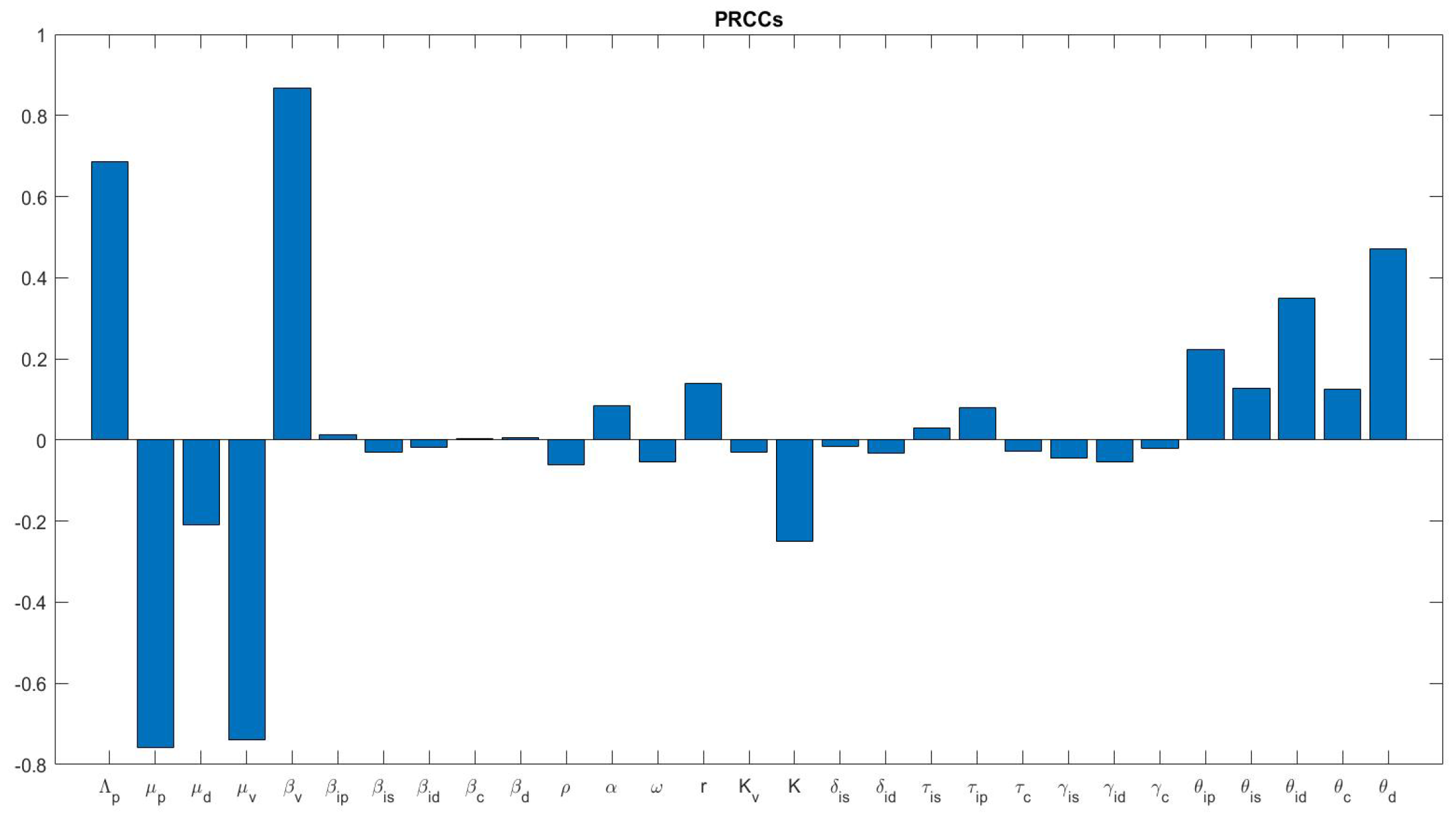
3.2.2. Global Sensitivity Analysis of ${\mathcal{R}}_c$

Since the model’s asymptotic analysis is entirely based on the control reproduction number $\left({\mathcal{R}}_c\right)$, we performed a global sensitivity analysis on ${\mathcal{R}}_c$ simultaneously changing the parameters (robustness analysis). Sensitivity analysis was then used to identify parameters that have a high impact on ${\mathcal{R}}_c$ and should be targeted to reduce animal (pig) mortality and morbidity due to African swine fever virus (ASFV). The Latin hypercube sampling (LHS) [39] and partial rank correlation coefficient (PRCC) methodology with the associated MATLAB code provided by [39] are used to perform a global uncertainty and sensitivity analysis.

Thus, assuming a uniform distribution over the range of biologically realistic values (between the minimum and maximum) of the parameters (listed in Table 5), the range of each parameter is split into 2000 equal sub-intervals, and 2000 model simulations are performed (the necessary number of simulations should satisfy $N>4/3K$, where N is the number of simulations and K is the number of parameters [40]). A Latin hypercube sampling (LHS) scheme [39,41] samples 2000 values at random without replacement for each input parameter, generating a Latin hypercube sampling matrix. Partial rank correlation coefficients (PRCCs) and the corresponding p-values are computed. An output is considered sensitive to input if the corresponding $PRCC$ is less than $-0.50$ or greater than $+0.50$, and the corresponding p-value is less than $5\%$. The results of this analysis, depicted in Figure 3, show parameters that strongly influence the dynamics of African swine fever infection, namely ${\Lambda }_p$, ${\mu }_p$, ${\mu }_v$, ${\beta }_v$, and ${\theta }_d$ with significant impact on the response function. Parameters ${\Lambda }_P$, ${\beta }_v$, and ${\theta }_d$ have a positive influence on the control reproduction number ${\mathcal{R}}_c$, which means an increase in these parameters implies an increase in the control reproduction number ${\mathcal{R}}_c$. While parameters ${\mu }_p$ and ${\mu }_v$ have a negative influence on the control reproduction number ${\mathcal{R}}_c$, which means an increase in these parameters implies a decrease in the basic reproduction number ${\mathcal{R}}_c$.

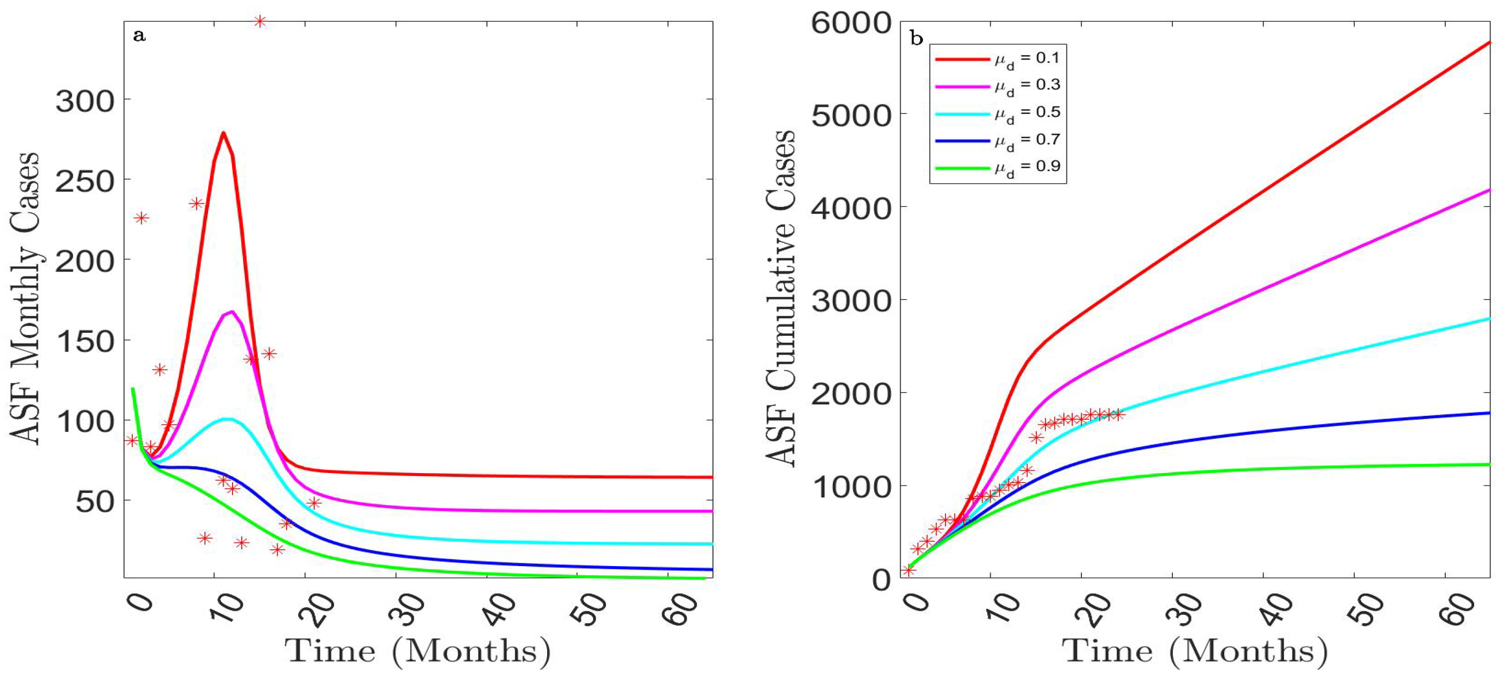
3.2.3. Assessing the Impact of the Burying or Cremation Rate of ASFV-Infected Dead Pigs, ${\mu }_d$

The proposed model 1 is simulated using the baseline parameter values in Table 5 to assess the impact of the burying or cremation rate of ASFV-infected dead pigs, ${\mu }_d$, on the dynamics of African swine fever virus (ASFV). The simulation results, depicted in Figure 4, show a significant decrease in the monthly (Figure 4a) and cumulative (Figure 4b) ASFV cases with an increase in the burying or cremation rate of ASFV-infected dead pigs, ${\mu }_d$. The figure indicates that increasing the burying or cremation rate of ASFV-infected dead pigs, ${\mu }_d$, by 30%, results in a 38% reduction in the monthly ASFV cases at the peak (Figure 4a). Moreover, nearly the same trend is observed when increasing the burying or cremation rate of ASFV-infected dead pigs, ${\mu }_d$ to 90%. Similar reductions are also observed in the monthly cumulative cases with an increasing rate of ${\mu }_d$ (Figure 4b). Consequently, in addition to control measures such as pig confinement and movement restrictions, as well as the culling of pigs on infected farms and in surrounding areas, as suggested by [15,16,17,18], proper burial or cremation of ASFV-infected dead pigs proves to be the most effective way to reduce ASFV transmission dynamics and contain outbreaks. However, effective measures for preventing and controlling African swine fever (ASF) infection require the active participation of all stakeholders in the pig industry.

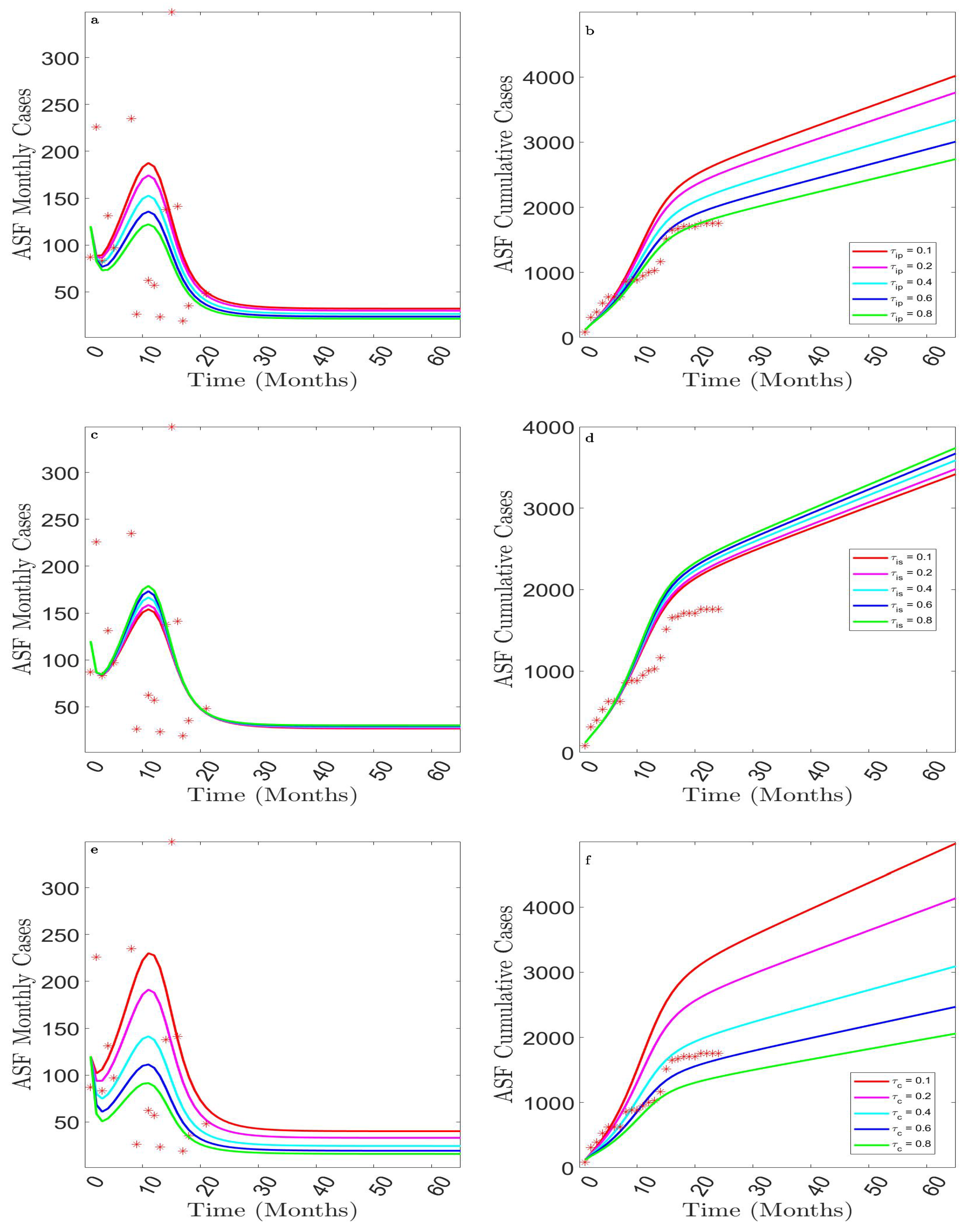
3.2.4. Assessing the Impact of Detecting Presymptomatic, Symptomatic, and Asymptomatic Cases

The proposed model 1 is further simulated to assess the impact of detecting presymptomatic, ${\tau }_{ip}$, symptomatic, ${\tau }_{is}$, and asymptomatic, ${\tau }_c$, cases on the dynamics of African swine fever virus (ASFV). The simulation results obtained, as depicted in Figure 5, show an increase in the monthly African swine fever virus (ASFV)-confirmed cases (Figure 5c) while increasing the detection of symptomatic infectious pigs in the population. A detection rate of symptomatic infectious at 60% shows that there is a 7% increase in the peak number of confirmed cases compared to a detection rate at 10% (cyan curve in Figure 5c). Also, if the detection rate increases to 80%, there is a 13% increase in the peak number of confirmed cases (green curve in Figure 5c). A similar increase is also observed in the monthly cumulative cases while increasing the rate of detection of infectious pigs in the population (Figure 5d). Therefore, early detection of infected pigs, coupled with the aforementioned control strategies, has the potential to minimize the spread of ASFV in the community. Thus, considering all these measures would enable the development of additional strategies to better control this disease.

4. Conclusions

African swine fever (ASF) is a contagious, virulent, inoculable, and highly fatal disease caused by the African swine fever virus (ASFV), affecting domestic pigs and wild boars. It spreads worldwide and threatens pig production, causing huge economic losses. The high morbidity and mortality associated with ASFV, the lack of an efficacious vaccine, and the complex makeup of the ASFV virion and genome, as well as its lifecycle, make this pathogen a serious threat to the global swine industry and national economies. To find a way to control this disease, we proposed integrating mathematical tools to study its transmission dynamics. Then, we formulated and analyzed a mathematical model for the transmission dynamics of African swine fever in Benin, considering the free-living virus in the environment. We proved that the model is well posed by showing some basic properties, and then we computed the control and the basic reproduction numbers (respectively ${\mathcal{R}}_c$ and ${\mathcal{R}}_0$). We provided the global attractivity of the disease-free equilibrium, showing that it is globally asymptotically stable when ${\mathcal{R}}_c<1$ and unstable when ${\mathcal{R}}_c>1$; the ASFV epidemic can be controlled effectively if the control reproduction number of the model can be brought to a value less than one and maintained. Finally, through numerical simulations, in the current situation, we found that ${\mathcal{R}}_0=2.78$, which implies that the disease will not die out without any control measures, and ${\mathcal{R}}_c=1.55$, showing that the eradication of the disease highly depends on the control measures taken to reduce disease transmission. A major issue with the model used is the under-reporting of infected pigs, which could bias model parameter estimation and lead to an underestimation of the reproduction number. It appears that early detection of infected pigs, coupled with proper burial or cremation of dead ASFV pigs, are key measures to prevent ASFV spread. Indeed, under-reporting is closely linked to the strategies in place for detecting infected pigs, which can introduce a varying reporting probability. Moreover, as more data become available, studying an ASFV model that captures breeders’ attitudes toward prophylactic (biosecurity) measures and the cost analysis of intervention strategies will be an interesting extension of this work.

References

1. Chenais, E.; Depner, K.; Guberti, V.; Dietze, K.; Viltrop, A.; Ståhl, K. Epidemiological considerations on African swine fever in Europe 2014–2018. Porc. Health Manag. 2019, 5, 1–10. [Google Scholar] [CrossRef] [PubMed]
2. Galindo, I.; Alonso, C. African swine fever virus: A review. Viruses 2017, 9, 103. [Google Scholar] [CrossRef] [PubMed]
3. Quembo, C.J.; Jori, F.; Vosloo, W.; Heath, L. Genetic characterization of african swine fever virus isolates from soft ticks at the wildlife/domestic interface in mozambique and identification of a novel genotype. Transbound. Emerg. Dis. 2018, 65, 420–431. [Google Scholar] [CrossRef] [PubMed]
4. Dixon, L.K.; Stahl, K.; Jori, F.; Vial, L.; Pfeiffer, D.U. African swine fever epidemiology and control. Annu. Rev. Anim. Biosci. 2020, 8, 221–246. [Google Scholar] [CrossRef] [PubMed]
5. Jurado, C.; Mur, L.; PérezAguirreburualde, M.S.; Cadenas-Fernández, E.; Martínez-López, B.; Sánchez-Vizcaíno, J.M.; Perez, A. Risk of african swine fever virus introduction into the united states through smuggling of pork in air passenger luggage. Sci. Rep. 2019, 9, 1–7. [Google Scholar] [CrossRef] [PubMed]
6. Montgomery, R.E. On a form of swine fever occurring in british east africa (kenya colony). J. Comp. Pathol. Ther. 1921, 34, 159–191. [Google Scholar] [CrossRef]
7. Penrith, M.-L.; Vosloo, W.; Jori, F.; Bastos, A.D. African swine fever virus eradication in africa. Virus Res. 2013, 173, 228–246. [Google Scholar] [CrossRef] [PubMed]
8. Mulumba-Mfumu, L.K.; Saegerman, C.; Dixon, L.K.; Madimba, K.C.; Kazadi, E.; Mukalakata, N.T.; Oura, C.A.; Chenais, E.; Masembe, C.; Ståhl, K.; et al. African swine fever: Update on eastern, central and southern africa. Transbound. Emerg. Dis. 2019, 66, 1462–1480. [Google Scholar] [CrossRef] [PubMed]
9. Arias, M.; Jurado, C.; Gallardo, C.; Fernández-Pinero, J.; Sánchez-Vizcaíno, J. Gaps in african swine fever: Analysis and priorities. Transbound. Emerg. Dis. 2018, 65, 235–247. [Google Scholar] [CrossRef]
10. Beltran-Alcrudo, D.; Falco, J.R.; Raizman, E.; Dietze, K. Transboundary spread of pig diseases: The role of international trade and travel. BMC Vet. Res. 2019, 15, 64. [Google Scholar] [CrossRef]
11. Fasina, F.O.; Kissinga, H.; Mlowe, F.; Mshang’a, S.; Matogo, B.; Mrema, A.; Mhagama, A.; Makungu, S.; Mtui-Malamsha, N.; Sallu, R.; et al. Drivers, risk factors and dynamics of african swine fever outbreaks, southern highlands, tanzania. Pathogens 2020, 9, 155. [Google Scholar] [CrossRef] [PubMed]
12. Sánchez-Cordón, P.; Montoya, M.; Reis, A.; Dixon, L. African swine fever: A re-emerging viral disease threatening the global pig industry. Vet. J. 2018, 233, 41–48. [Google Scholar] [CrossRef] [PubMed]
13. Wang, N.; Zhao, D.; Wang, J.; Zhang, Y.; Wang, M.; Gao, Y.; Li, F.; Wang, J.; Bu, Z.; Rao, Z.; et al. Architecture of african swine fever virus and implications for viral assembly. Science 2019, 526, 110798. [Google Scholar] [CrossRef] [PubMed]
14. Calkins, C.M.; Scasta, J.D. Transboundary animal diseases (tads) affecting domestic and wild African ungulates: African swine fever, foot and mouth disease, rift valley fever (1996–2018). Res. Vet. Sci. 2020, 131, 69–77. [Google Scholar] [CrossRef] [PubMed]
15. Arias, M.; Sánchez-Vizcaíno, J.M.; Morilla, A.; Yoon, K.; Zimmerman, J. African swine fever. In Trends in Emerging Viral Infections of Swine; Wiley: Hoboken, NJ, USA, 2002; pp. 119–124. [Google Scholar]
16. Barasona, J.A.; Gallardo, C.; Cadenas-Fernández, E.; Jurado, C.; Rivera, B.; Rodríguez-Bertos, A.; Arias, M.; Sánchez-Vizcaíno, J.M. First oral vaccination of eurasian wild boar against African swine fever virus genotype ii. Front. Vet. Sci. 2019, 6, 137. [Google Scholar] [CrossRef] [PubMed]
17. Morilla, A.; Yoon, K.-J.; Zimmerman, J.J. Trends in Emerging Viral Infections of Swine; John Wiley & Sons: Hoboken, NJ, USA, 2008. [Google Scholar]
18. Sánchez, E.G.; Pérez-Núñez, D.; Revilla, Y. Development of vaccines against african swine fever virus. Virus Res. 2019, 265, 150–155. [Google Scholar] [CrossRef] [PubMed]
19. de Carvalho Ferreira, H.; Backer, J.; Weesendorp, E.; Klinkenberg, D.; Stegeman, J.; Loeffen, W. Transmission rate of african swine fever virus under experimental conditions. Vet. Microbiol. 2013, 165, 296–304. [Google Scholar] [CrossRef] [PubMed]
20. Gulenkin, V.; Korennoy, F.; Karaulov, A.; Dudnikov, S. Cartographical analysis of african swine fever outbreaks in the territory of the russian federation and computer modeling of the basic reproduction ratio. Prev. Vet. Med. 2011, 102, 167–174. [Google Scholar] [CrossRef]
21. Lange, M.; Guberti, V.; Thulke, H.-H. Understanding asf spread and emergency control concepts in wild boar populations using individual-based modelling and spatio-temporal surveillance data. EFSA Support. Publ. 2018, 15, 1521E. [Google Scholar] [CrossRef]
22. Loi, F.; Cappai, S.; Laddomada, A.; Feliziani, F.; Oggiano, A.; Franzoni, G.; Rolesu, S.; Guberti, V. Mathematical approach to estimating the main epidemiological parameters of african swine fever in wild boar. Vaccines 2020, 8, 521. [Google Scholar] [CrossRef]
23. Pietschmann, J.; Guinat, C.; Beer, M.; Pronin, V.; Tauscher, K.; Petrov, A.; Keil, G.; Blome, S. Course and transmission characteristics of oral low-dose infection of domestic pigs and european wild boar with a caucasian african swine fever virus isolate. Arch. Virol. 2015, 160, 1657–1667. [Google Scholar] [CrossRef]
24. Barongo, M.B.; Bishop, R.P.; Fèvre, E.M.; Knobel, D.L.; Ssematimba, A. A mathematical model that simulates control options for African swine fever virus (asfv). PLoS ONE 2016, 11, e0158658. [Google Scholar] [CrossRef] [PubMed]
25. Gervasi, V.; Marcon, A.; Bellini, S.; Guberti, V. Evaluation of the efficiency of active and passive surveillance in the detection of african swine fever in wild boar. Vet. Sci. 2019, 7, 5. [Google Scholar] [CrossRef]
26. Halasa, T.; Bøtner, A.; Mortensen, S.; Christensen, H.; Toft, N.; Boklund, A. Simulating the epidemiological and economic effects of an african swine fever epidemic in industrialized swine populations. Vet. Microbiol. 2016, 193, 7–16. [Google Scholar] [CrossRef]
27. EFSA Panel on Animal Health and Welfare (AHAW); More, S.; Miranda, M.A.; Bicout, D.; Bøtner, A.; Butterworth, A.; Calistri, P.; Edwards, S.; Garin-Bastuji, B.; Good, M.; et al. African swine fever in wild boar. EFSA J. 2018, 16, e05344. [Google Scholar]
28. Van den Driessche, P.; Watmough, J. Reproduction numbers and sub-threshold endemic equilibria for compartmental models of disease transmission. Math. Biosci. 2002, 180, 29–48. [Google Scholar] [CrossRef] [PubMed]
29. Bani-Yaghoub, M.; Gautam, R.; Shuai, Z.; Van DenDriessche, P.; Ivanek, R. Reproduction numbers for infections with free-living pathogens growing in the environment. J. Biol. Dyn. 2012, 6, 923–940. [Google Scholar] [CrossRef]
30. Li, M.Y.; Graef, J.R.; Wang, L.; Karsai, J. Global dynamics of a seir model with varying total population size. Math. Biosci. 1999, 160, 191–213. [Google Scholar] [CrossRef] [PubMed]
31. Kamgang, J.C.; Sallet, G. Computation of threshold conditions for epidemiological models and global stability of the disease-free equilibrium (dfe). Math. Biosci. 2008, 213, 1–12. [Google Scholar] [CrossRef]
32. Lakshmikantham, V.; Leela, S.; Martynyuk, A.A. Stability Analysis of Nonlinear Systems; Springer: Berlin/Heidelberg, Germany, 1989. [Google Scholar]
33. Smith, H.L. Monotone Dynamical Systems: An Introduction to the Theory of Competitive and Cooperative Systems: An Introduction to the Theory of Competitive and Cooperative Systems; Number 41; American Mathematical Society: Ann Arbor, MI, USA, 2008. [Google Scholar]
34. Castillo-Chavez, C.; Thieme, H. Asymptotically autonomous epidemic models. In Mathematical Population Dynamics: Analysis of Heterogeneity; Wuerz Publishing Ltd.: Winnipeg, MB, Canada, 1994. [Google Scholar]
35. Castillo-Chavez, C.; Song, B. Dynamical models of tuberculosis and their applications. Math. Biosci. Eng. 2004, 1, 361. [Google Scholar] [CrossRef]
36. Carr, J. Applications of Center Manifold Theory; Springer: New York, NY, USA; Heidelberg/Berlin, Germany, 1981. [Google Scholar]
37. Song, H.; Li, J.; Jin, Z. Nonlinear dynamic modeling and analysis of african swine fever with culling in china. Commun. Nonlinear Sci. Numer. Simul. 2023, 117, 106915. [Google Scholar] [CrossRef]
38. Zhang, X.; Rong, X.; Li, J.; Fan, M.; Wang, Y.; Sun, X.; Huang, B.; Zhu, H. Modeling the outbreak and control of african swine fever virus in large-scale pig farms. J. Theor. Biol. 2021, 526, 110798. [Google Scholar] [CrossRef] [PubMed]
39. Marino, S.; Hogue, I.B.; Ray, C.J.; Kirschner, D.E. A methodology for performing global uncertainty and sensitivity analysis in systems biology. J. Theor. Biol. 2008, 254, 178–196. [Google Scholar] [CrossRef] [PubMed]
40. McKay, M.D.; Beckman, R.J.; Conover, W.J. A comparison of three methods for selecting values of input variables in the analysis of output from a computer code. Technometrics 2000, 42, 55–61. [Google Scholar] [CrossRef]
41. Blower, S.M.; Dowlatabadi, H. Sensitivity and uncertainty analysis of complex models of disease transmission: An HIV model, as an example. In International Statistical Review/Revue Internationale de Statistique; Wiley: Hoboken, NJ, USA, 1994; pp. 229–243. [Google Scholar]
Figure 1. Flow diagram for the dynamic of African Swine Fever.
Mathematics 12 01749 g001
Figure 2. Model fitting to the cumulative new reported cases of ASF from January 2020 to December 2021.
Mathematics 12 01749 g002
Figure 3. Partial rank correlation coefficients (PRCCs).
Mathematics 12 01749 g003
Figure 4. Impact of the burying or cremation rate of ASFV-infected dead pigs, μ d , on the new monthly ASF cases (a) and the cumulative monthly ASF cases (b). *: reported cases.
Mathematics 12 01749 g004
Figure 5. Impact of detecting presymptomatic (a,b), symptomatic (c,d) and asymptomatic (e,f) cases. *: reported cases.
Mathematics 12 01749 g005