A Numerical Analysis of the Non-Uniform Layered Ground Vibration Caused by a Moving Railway Load Using an Efficient Frequency–Wave-Number Method

Abstract

The ground vibration caused by the operation of high-speed trains has become a key challenge in the development of high-speed railways. In order to study the train-induced ground vibration affected by geotechnical heterogeneity, an efficient frequency–wave-number method coupled with the random variable theory model is proposed to quickly obtain the numerical results without losing accuracy. The track is regarded as a composite Euler–Bernoulli beam resting on the layered ground, and the spatial heterogeneity of the ground soil is considered. The ground dynamic characteristics of an elastic, layered, non-uniform foundation are investigated, and numerical results at three typical train speeds are reported based on the developed Fortran computer programs. The results show that as the soil homogeneity coefficient increases, the peak acceleration continuously decreases in the transonic case, while it gradually increases in the supersonic case, and the ground acceleration spectrum at a far distance obviously decreases; the maximum acceleration occurs at the track edge, and a local rebound in vibration attenuation occurs in the supersonic case.

1. Introduction

The high-speed train (HST) has become a convenient method of passenger transport in China in recent years. The ground vibration caused by HSTs near track facilities propagates far through the ground surface, affecting people’s lives and the normal use of precision instruments along the operation line [1]. Train-induced environmental vibrations have become a key challenge in the development of HSTs in terms of railway administrative organization.

Vibrations induced by moving quasi-static train loads have been extensively investigated for several decades. Beskou and Theodorakopoulos [2] detailedly reviewed the dynamic response of road pavements to moving loads on their surface, exploring aspects ranging from the load/track/foundation soil model to the analysis method to the coupled dynamic system. In that review paper, a large number of different types of methods were reviewed, including frequency-domain methods, together with the effect of soil properties on the response of railway line vibrations. The foundation can be modeled by a homogeneous or layered half-space, which can usually be described as an elastic, saturated, or even unsaturated poro-elastic medium [3,4,5,6,7]. Generally speaking, there are a total of three kinds of solution methods for dealing with this subject, i.e., analytical methods [8,9], purely numerical methods (such as FEM and BEM) [10,11], and semi-analytical methods [12,13,14], under conditions of plane strain or full three-dimensionality. However, analytical approaches cannot readily obtain close-formed solutions for complex conditions; as for the numerical method, the simplified plane strain model cannot accurately simulate the Mach radiation effect of wave propagation despite a higher calculation speed; finally, the three-dimensional model is time-consuming and often leads to large computational storage, just because of the high speed of about 300 km/h. To date, many efforts have been made to overcome the drawbacks of the above methods. Assuming the material and geometric properties to be constant along the train’s moving direction, the 3D problem can be transformed into the frequency–wave-number domain by applying the Fourier transform to time and variables in the moving direction. Such an idea was first used to study the response of an underground structure to traveling seismic waves [15,16]. This numerical concept was also adopted by some scholars [17,18,19,20,21] to quickly evaluate the dynamic vibration of the elastic uniform/layered ground under moving train loads. The authors in [1,7,22] generalized this method to solve the unsaturated ground vibration caused by an HST. In this semi-numerical calculation model, finite element discretization is only required in the section perpendicular to the track, and the governing equations are solved in the frequency–wave-number plane; hence, relatively high numerical accuracy can be acquired with little computational effort [23].

It is noteworthy that in most previous studies concerning train-induced ground vibrations, the granular soil is usually limited to the assumption of an isotropic elastic medium, and the physical/mechanical characteristics are assumed to be uniform in the calculation model [4,5,6,7,9,10,11,12,13,14,17,18,19,20,21,22]. However, in geotechnical practice, it is well known that the physical/mechanical properties of the ground soil are uncertain or variable with inherent randomness and have strong non-uniformity [24]. As pointed out by Dieterman [12] and Sheng [13], soil characteristics have a significant effect on the vibration characteristics of the ground, especially at high train speeds. In order to make reliable predictions of vibration propagation and attenuation, soil spatial variability should certainly be considered in the numerical study of train-caused environmental vibrations. To date, although lots of attention has been paid to soil spatial variability in research on slope stability, seismic analysis, foundation bearing capacity, and deformation [25,26,27,28,29,30,31,32], little attention has been paid to elucidating the effect of soil non-uniformity on the environmental vibration caused by a moving train. Gao et al. [33] analyzed the vibrations caused by HSTs on a non-homogeneous foundation by using a semi-analytical boundary-element-coupled thin-layer method and pointed out that the vertical and horizontal vibrations are influenced by the vertical non-uniformity coefficient of the foundation soil, which should be paid attention to in the vibration isolation design. Zhou et al. [34,35] studied the vibration of a graded non-uniform foundation under a rectangular moving load in which the soil shear modulus linearly varied with depth, and the results showed that the vertical soil displacement decreased proportionally with the surface shear modulus, non-homogeneity degree, and load velocity. Ma et al. [36] and Shi et al. [37] established a graded non-homogeneous elastic/unsaturated foundation model and analyzed the impact of ground non-homogeneity by the semi-numerical back-propagation ray matrix method and Helmholtz decomposition, concluding that the vertical displacement decreases with the increase in the gradient factor. These studies indicate that the non-uniformity of the foundation soil is of great significance and worth considering to understand the special characteristics and the propagation of foundation vibrations.

The purpose and novelty of this paper are the establishment of a numerical procedure framework for dealing with train-induced ground vibrations, with consideration of soil spatial variability. An efficient frequency–wave-number method is proposed to numerically study layered ground vibration with soil non-homogeneity under an HST load. Random variable theory is incorporated into a semi-numerical model to represent the spatial heterogeneity of the ground soil. The track is regarded as a composite Euler beam, and the Fortran computer program is developed based on the presented model to solve the equation system in the frequency–wave-number domain. The ground vibration can be quickly and accurately derived by using an appropriate frequency range, which can significantly overcome the drawbacks of time consumption and large computational storage. Finally, the ground dynamic characteristics of an elastic, layered, non-uniform foundation are investigated, in which the spatial non-homogeneity of the surface foundation is considered. Numerical studies at three typical speeds, i.e., the subsonic, transonic, and supersonic cases, are conducted to consider the speed effect.

2. Solution Method and Verification

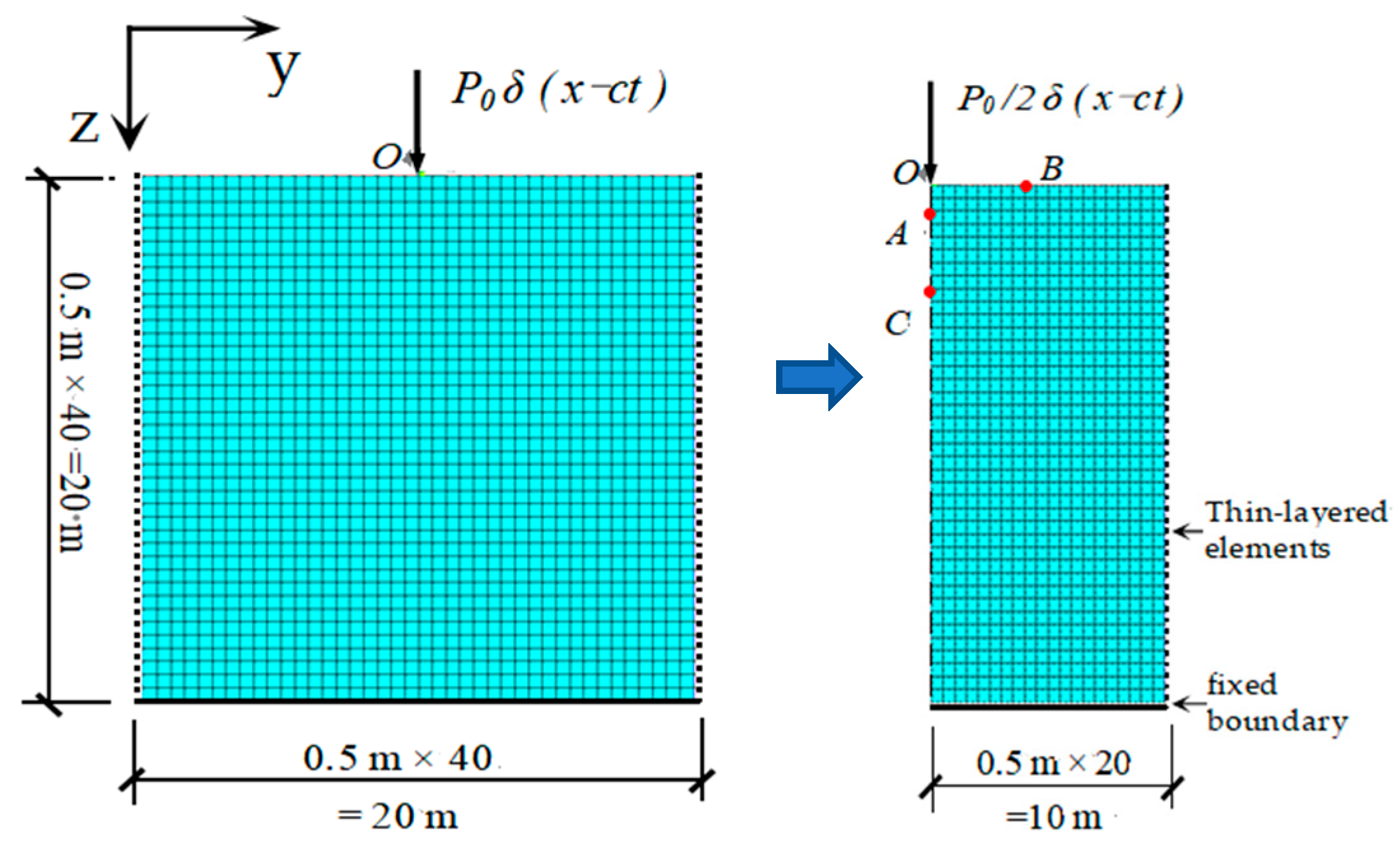
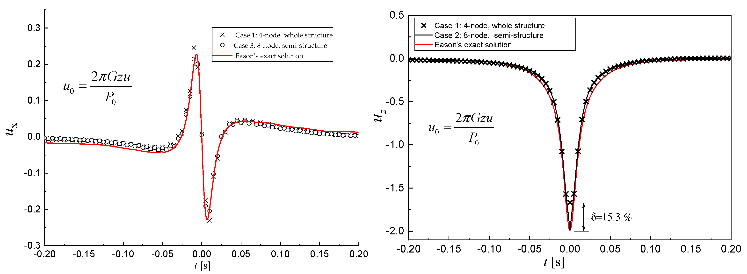
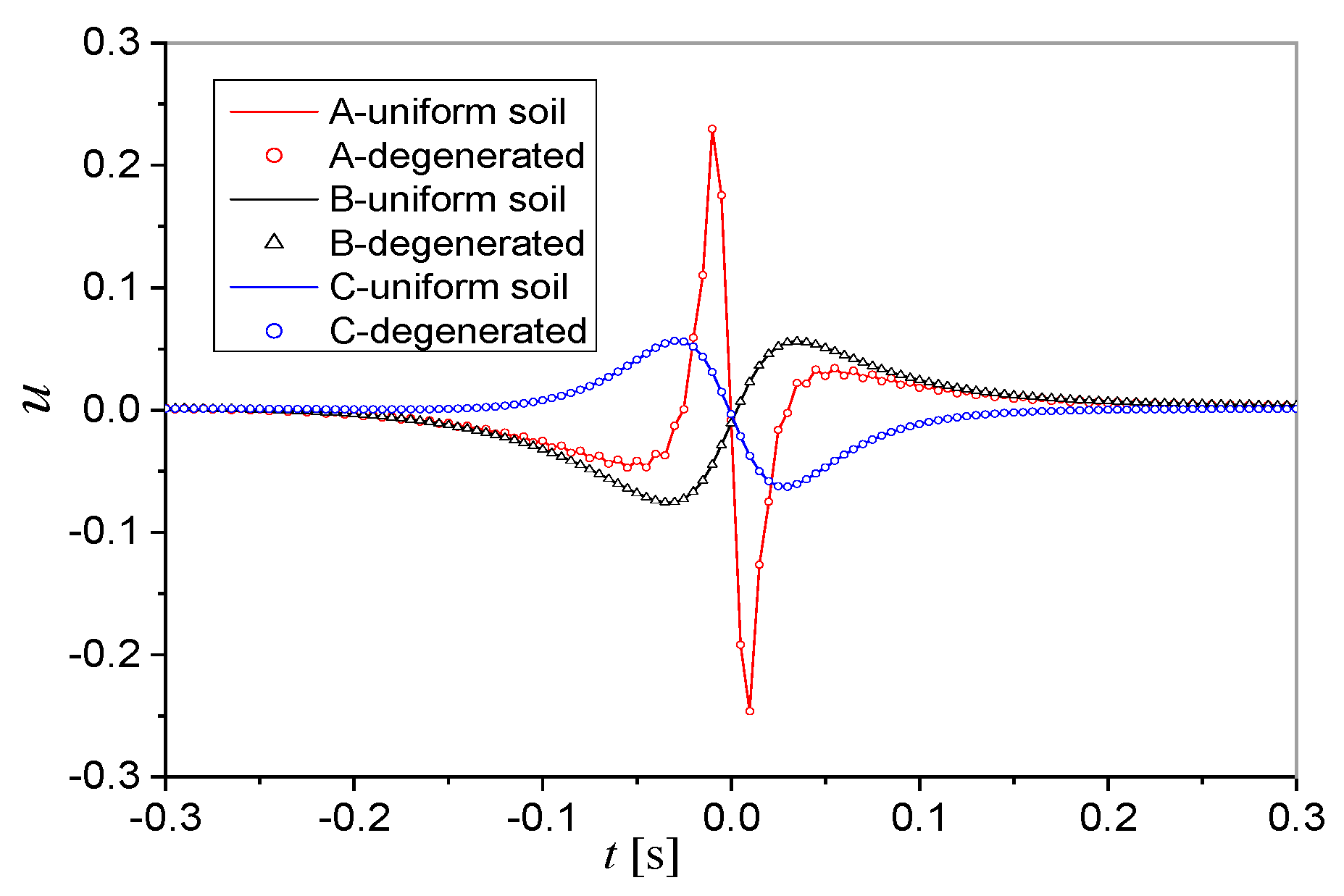
2.1. Basic Frequency–Wave-Number Method for Uniform Soil and Program Verification

In elastodynamic theory, when the Fourier transform is performed on the time term in Navier’s equation in the absence of a body force, the equation of motion in the frequency domain can be expressed as [18]

$${\mu }^c{\tilde{u}}_{i,jj}+({\lambda }^c+{\mu }^c){\tilde{u}}_{j,ij}+{\omega }^2\rho {\tilde{u}}_i=0$$

(1)

where u_i denotes the displacement components of a material point, subscripts i and j are defined here as notations for Cartesian components, $\omega$ is the excitation frequency, ρ is the material density, and λ^c and μ^c are complex Lame constants considering the soil hysteresis damping of wave propagation [17,18]. Variables with the superscript ‘~’ represent components in the frequency domain.

In addition, when the Galerkin method and partial integration are applied to the equilibrium equation and stress boundary condition in elastic theory, the principle of virtual work in the frequency domain can be obtained as follows:

$${\displaystyle {\int }_V\delta }{\tilde{\epsilon }}_{ij}^{*}{\tilde{\sigma }}_{ij}dv={\displaystyle {\int }_V\rho {\omega }^2\delta {\tilde{u}}_i^{*}}{\tilde{u}}_{i}dv+{\displaystyle {\int }_{S^{\sigma }}\delta {\tilde{u}}_i^{*}}{\tilde{f}}_{i}dS$$

(2)

where ε_ij and σ_ij are the Cauchy strain and stress tensor, respectively;and f_i is the Cauchy traction vector at a point on boundary S^σ. The geometric shape and material properties of elastic soil are assumed to be unchanged along the moving direction. Equations (1) and (2) are in the frequency–3D-space domain V. When the Fourier transform is applied to the variable x in Equation (2), it can be transformed into the frequency–2D-wave-number domain S in a matrix form:

$${\displaystyle {\int }_S\delta {\tilde{\overline{\epsilon }}}^{*T}}\tilde{\overline{\sigma }}dS={\displaystyle {\int }_S\rho {\omega }^2}\delta {\tilde{\overline{u}}}^{*T}\tilde{\overline{u}}dS+{\displaystyle {\int }_{S^{\sigma }}\delta {\tilde{\overline{u}}}^{*T}}\tilde{\overline{f}}dS$$

(3)

where the superscript ‘T’ represents the transpose of the matrix, and variables with the superscript ‘⋍’ represent components in the frequency–wave-number domain. Substituting the geometric equations and constitutive equations in the frequency–wave-number domain into Equation (3) yields the final governing formulation of the elastic medium in the frequency–wave-number domain in a matrix form:

$$(K-{\omega }^{2}M)\times \tilde{\overline{U}}=F$$

(4)

where the stiffness matrix, mass matrix, and external equivalent nodal load vector can be respectively expressed as

$$\begin{gathered} K={\displaystyle \sum _e{\displaystyle {\int }_{-1}^1{\displaystyle {\int }_{-1}^1{(B^{*}N)}^{T}D(BN)\left|J\right|d\eta d\xi }}} \\ M={\displaystyle \sum _e{\rho }^e{\displaystyle {\int }_{-1}^1{\displaystyle {\int }_{-1}^1{N}^T}}N\left|J\right|d\eta d\xi } \\ F={\displaystyle \sum _e{\displaystyle {\int }_{-1}^1{\displaystyle {\int }_{-1}^1{N}^T\tilde{\overline{f}}\left|J\right|d\eta d\xi }}} \end{gathered}$$

in which B is the partial derivative matrix, and D is the stress matrix of the elastic medium in the frequency–wave-number domain, as depicted in [19,20]; the superscript ‘*’ represents the conjugate of a matrix, J is the Jacobi matrix, f is the equivalent nodal load vector, N is the shape function of an 8-node quadrilateral isoparametric finite element, $\eta \mathrm{a}\mathrm{n}\mathrm{d}\xi$ are local coordinates in the finite element, and ${\eta }_i\mathrm{a}\mathrm{n}\mathrm{d}{\xi }_i$ are nodal coefficients. Readers can refer to the previous literature [19,20,21] for the detailed derivation process and parameter meanings. Note that soil homogeneity can be considered in the D matrix since its elements are related to the elastic modulus E and Poisson’s ratio v. This issue will be detailedly discussed in Section 2.3 hereinafter.

Governing Equation (4) is a linear equation system with complex coefficients and has a unique solution for the given boundary conditions. The solution will be obtained by solving the linear equation system in the frequency–wave-number domain. By using the double inverse fast Fourier transform, we can obtain results in the time–space domain.

For uniform 3D homogeneous ground, the analytical solution derived by Eason [8] for a half-space under a moving point force was adopted to verify the proposed frequency–wave-number method and the corresponding Fortran programs. The density is 2000 kg/m³, Poisson’s ratio is 0.25, and the soil damping coefficient and shear wave speed are 0.05 and 100 m/s, respectively. The elastic modulus of the half-space is 50 MPa. The half-space is approximated by uniform soil layers resting on a rigid rock layer, and the point load applied in the z-direction has a moving speed of 90 m/s in the x-direction. The direction definition here will be adopted throughout the numerical studies. The transversal vertical section is meshed by finite elements in the near field of the ground, and thin-layered elements [38] are set at the boundaries to absorb the external wave caused by the moving train. A fixed boundary is used at the bottom of the 20 m × 20 m model, which can be reduced to a semi-structure of 10 m × 20 m due to the symmetry of the structure, as shown in Figure 1. The finite element size is 0.5 m × 0.5 m, and the nodes and elements are re-numbered in a new pattern in the direction from the top left to the bottom right after extracting the information from the Abaqus pre-processing module. The degrees of freedom for the bottom fixed nodes are constrained in the programming process, and the dynamic response of point A, located at coordinate (0, 0, −1), is studied. The normalized displacements in both the z- and x-directions are presented in Figure 2 in comparison with an analytical solution [8]. The time t = 0 corresponds to the instant at which the point load passes through the profile x = 0. It can be seen that the displacement in the z-direction is much greater than that in the x-direction. The results of the 4-node isoparametric finite element with the whole structure are also depicted for comparison. The three solutions are in good agreement; however, the 4-node element scheme has a 20% gap with the analytical one, and the 8-node element scheme with the semi-structure is closer to the analytical values. This scheme significantly reduces the computational cost without losing numerical accuracy, indicating the reliability of the proposed method and the corresponding program.

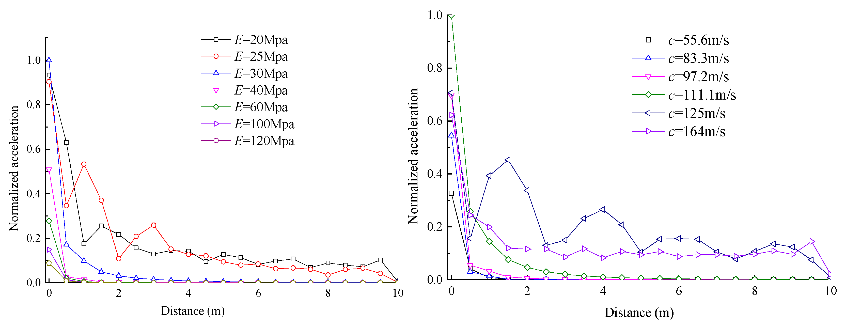
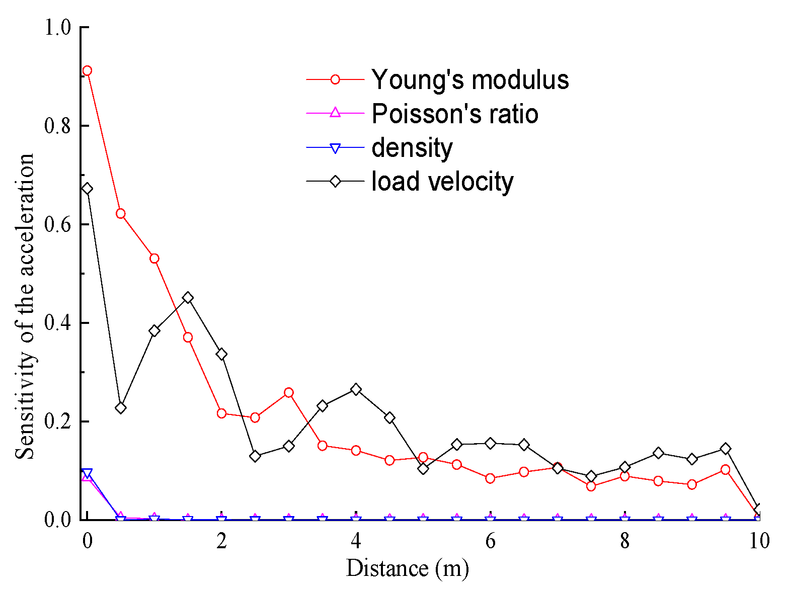
2.2. Finding the Key Factors Affecting the Foundation Vibrations Caused by a Moving Load

In order to choose the appropriate calculation parameters when considering soil homogeneity, we need to find the key factors affecting the dynamic response of the foundation. Therefore, the basic frequency–wave-number method and geometric model for uniform ground in Section 2.1 are now used to study the response and attenuation to find the key factors. The benchmark values of soil physical parameters, i.e., Young’s modulus, Poisson’s ratio, soil density, and load speed, are listed in

Table 1. Benchmark values and parameter ranges in the simulation to find key factors influencing the ground vibration [20,39].

Parameters	Young’s Modulus (MPa)	Poisson’s Ratio	Density (kg/m3)	Load Velocity (m/s)
Benchmark value	50	0.25	2000	100.0
Variation range	[20, 120]	[0.20, 0.45]	[1300, 2300]	[55.6, 164.0]

, which are arranged on the basis of [20]. We take a wide parameter range approximately centered around the benchmark value to find the extent to which their changes affect the calculation results. The variation ranges of typical soil parameters are taken from [39]. The benchmark value remains unchanged unless otherwise specified. The Rayleigh and shear wave velocities corresponding to the benchmark parameters are 114 m/s and 124 m/s, respectively. The detailed calculation parameters are listed in

Table 2. Detailed values of calculation parameters for ground vibration simulation.

Young’s Modulus (MPa)	Poisson’s Ratio	Density (kg/m3)	Load Velocity (m/s)
20	0.20	1300	55.6
25	0.23	1500	83.3
40	0.25	1700	97.2
60	0.30	1900	111.1
100	0.35	2100	125.0
120	0.45	2300	164.0

. The observation points are located on the foundation surface at intervals of 0.5 m.

The attenuation rate of the normalized ground displacement amplitude in the x- and z-directions can be seen in Figure 3. Here, z means the direction in which the vertical load is applied, and x means the load’s moving direction. The displacement in the z-direction decays faster with the distance than that in the x-direction within 6 m from the moving load. The attenuation of the normalized ground acceleration is shown in Figure 4 as soil parameters and load velocity vary, as specified in Table 2. To quantitatively judge the influencing degree of the parameters, the sensitivity of the normalized ground acceleration was used [39,40]. Here, sensitivity is defined by the following equation with the change rate of the input parameter x_i:

$${\eta }_{ss}={\eta }_{sr}\times \frac{\max x_r-\min x_r}{x}=\raisebox{1ex}{$\frac{y_i-y_0}{y_0}$}\!\left/ \!\raisebox{-1ex}{$\frac{x_i-x_0}{x_0}$}\right.\times \frac{\max x_r-\min x_r}{x_i}$$

(5)

where η_ss and η_ss are sensitivity and the sensitivity coefficient, respectively; x_r is the range of the parameter; x₀ is the benchmark value listed in Table 1; and x_i and y_i are the parameters listed in Table 2 and the corresponding ground acceleration, respectively. The first simulation is performed using the benchmark values of the parameters. Then, six sets of simulations are performed to investigate the sensitivity of each parameter to the ground vibration. The sensitivity results are shown in Figure 5. It can be clearly observed in Figure 4 and Figure 5 that, among the physical and mechanical parameters of the soil, the elastic modulus has enormous implications, together with the speed of the moving load, while Poisson’s ratio and the soil density have negligible effects on the ground vibration. This finding is consistent with the previous study in [39]. Therefore, the elastic modulus is chosen as the key factor when considering soil homogeneity, and the train speed should also be considered. Hereinafter, the influence of spatial homogeneity on the soil elastic modulus at different speeds of an HST will be studied, and Poisson’s ratio and the density are regarded as deterministic.

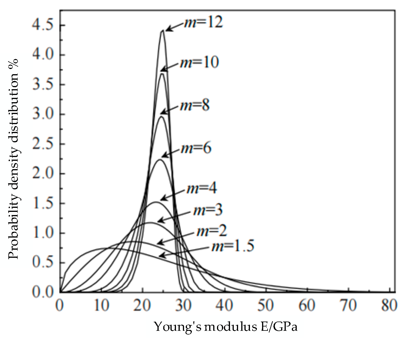
2.3. Random Model Considering Soil Spatial Variability and Program Verification

On the basis of Section 2.1 and Section 2.2, we now consider embedding the soil homogeneity model in the basic frequency–wave-number method. Random variable theory is a widely used method in geotechnical practice for considering soil non-uniformity due to its high calculation efficiency compared to field theory [24,25]. To investigate the influence of soil spatial heterogeneity on ground-wave propagation, random variable theory and the Monte Carlo approach were used by Coelho et al. in [32] and showed a significant reduction in the computational cost; therefore, in the present study, random variable theory is adopted to represent the spatial variability of ground soil. The D matrix in Equation (4) considers the interior elastic parameters of soil elements to be uniform, while each element is distributed independently with the randomized elastic modulus E. The Young’s modulus of each soil element changes with its spatial position, and its statistical distribution can be described by the Weibull function [41]. Therefore, the Weibull statistical distribution function is used to describe the modulus probability distribution of each soil element [41]:

$$f(E)=\frac{m}{E_0}{\left(\frac{E}{E_0}\right)}^{m-1}exp\left(-{\left(\frac{E}{E_0}\right)}^m\right)$$

(6)

where E is the elastic modulus of the soil element, E₀ is the mean value, and m is the shape parameter. It is the elastic modulus of the soil element here that enables us to consider the spatial variability in the following numerical calculation. This relationship is then directly incorporated into the frequency–wave-number method previously proposed in Section 2.1 to give consideration to the ground non-uniformity. The probability density function is shown in Figure 6. It can be seen that the probability density is strongly influenced by the shape parameter m. A larger value of m means a higher homogeneity level, and when m tends is large enough (such as 150), the soil becomes homogeneous. When the shape parameter takes smaller values, such as 2, the elastic modulus parameters of the soil element are distributed in quite a wide range, indicating a weak uniformity of the foundation soil. An m value exceeding 12 indicates a higher level of homogeneity of the foundation soil. In the common situation, a median value of m, such as 5, can be chosen. At each specific m value (homogeneity coefficient) in the numerical analysis, sufficient automatic Monte Carlo (MC) simulations were adopted to generate random parameters, which have a convergent probability mean value of E₀. The produced parameters with a non-uniform distribution would serve as parameter fields in numerical simulations at each specific homogeneity coefficient.

The applicability of the program developed in this section, i.e., the frequency–wave-number method coupled with the random model, needs to be numerically evaluated. We degenerate the coupled non-uniform model into a uniform one by setting m to a large enough value (200), and the existing analytical solution [8] for a uniform elastic half-space is used to illustrate the proposed framework. The displacements of the A, B, and C points in Section 2.1 are compared with the uniform ones [8], as shown in Figure 7. Still, the time t = 0 corresponds to the instant at which the point load passes through the profile x = 0. It can be seen that all displacements with the degenerated uniform model are in good agreement with the uniform model, illustrating the reliability of the present coupled non-uniform random model.

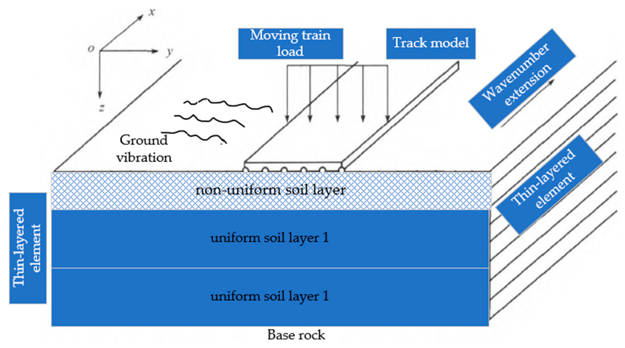
3. Analysis Model of Track and Non-Uniform Layered Ground

The track system consists of rails, fasteners, track panels, a CA mortar layer, a concrete base, and a subgrade. The track slab has an important effect on the track and ground vibrations. Here, we assume that the rails and the embankment beneath them have an overall deformation when acted on by the moving HST loads when investigating the ground vibration. Therefore, it is now described as a composite Euler beam [20,22]. The dynamic equation under a load p₀δ(x − ct) in the frequency–wave-number domain can be expressed as [22]

$$(EI{\xi }_x^4-m_c{\omega }^4){\tilde{\overline{u}}}_r={\tilde{\overline{f}}}_{IT}({\xi }_x,\omega )+{\tilde{\overline{p}}}_0({\xi }_x,\omega )$$

(7)

where ξ_x is the wave-number variable corresponding to the load’s moving direction x, m_c is the comprehensive mass of the track system, EI is its bending stiffness, u_r is the track displacement, p₀ is the external HST load, and f_IT is the reactive force at contact points of the ground surface; the superscript ‘⋍’ represents variables in the frequency–wave-number domain. The coupled track–non-uniform-ground model under a moving load can be described by combining Equations (4), (6) and (7).

We consider a typical HST in China comprising N cars with two bogies in each car (four pairs of wheels). In the frequency–wave-number domain, the moving loads of the train wheels acting on the track system can be directly mathematically described as follows [22]:

$$\tilde{\overline{p}}({\xi }_x,y,z,\omega )=\frac{2\pi }{V_c}\delta ({\xi }_x-\frac{\omega }{V_c})\chi ({\xi }_x)$$

(8)

where $\chi ({\xi }_x)={\displaystyle \sum _{n=1}^{N-1}[P_{n1}(1+exp(-i{a}_n{\xi }_x)+P_{n2}(exp(-i(a_n+b_n){\xi }_x)+exp(-i(2a_n+b_n){\xi }_x)]exp(-i{\displaystyle \sum _{k=0}^{N-1}{L}_k{\xi }_x})}$, V_c is the train’s moving velocity along the x-direction, δ (∙) denotes Dirac’s delta function, P_n1 is the front axle load and P_n2 is the rear axle load of the bogies, and a_n and b_n are the distances between axles. L_i is the ith car length, and L₀ is the distance to a reference position ahead of the first axle load position. The detailed parameters can be found in the authors’ previous paper in [22].

Figure 8 is a schematic diagram showing the interaction mechanism of the Euler track and non-uniform soil layers under a moving HST load. The cross-section of the soil perpendicular to the moving load in the frequency–wave-number plane is discretized using 8-node isoparametric elements. A semi-structure is adopted in the numerical calculation due to the symmetry, and thin-layered elements are set as wave-absorbing boundaries to reduce the reflection of the external traveling waves in the computational domain [33,38]. During the numerical simulation, the moving HST loads in the frequency–wave-number form can be directly applied to the points located at the contact surface between the Euler track and ground soil. Large-scale governing equations in the frequency–wave-number domain can be solved using the Gaussian elimination method. To obtain the dynamic response in the time–space domain, the double inverse fast Fourier transform is performed with respect to ξ_x and $\omega$, and it can be simplified to a single inverse fast Fourier transform due to the property of the Dirac function, which certainly improves the calculation efficiency. The inverse transform is performed using appropriate quadrature routines available in Fortran IMSL 5.0 (International Mathematics and Statistics Library).

4. Numerical Results of the Ground Vibration at Different Train Speeds and Homogeneity

Table 3. Numerical parameters of stratified foundation with non-homogeneous superficial soil [42].

Soil Layer No.	Thickness (m)	Shear Wave Velocity (m/s)	Density (kg/m3)	Poisson’s Ratio	Damping Coefficient	Mean Value of Elastic Modulus (107 pa)	Homogeneity Coefficient β	Shear Modulus (107 pa)
1	2	95	1500	0.35	0.05	3.66	2, 5, 15	1.35
2	2	150	1700	0.30	0.05	9.95	200	3.83
3	26	280	1800	0.25	0.05	35.28	200	14.11

lists the numerical parameters of the stratified foundation with non-homogeneous superficial soil [42]. Here, we use β to denote the homogeneity coefficient of the soil elastic modulus, with three representative values indicating different levels of soil non-uniformity. In practical geotechnical engineering, when the ground has ordinary and better uniformity, the homogeneity coefficient is in the range of 2–5, and for excellent ground soil after effective treatment and improvement, the coefficient can be increased to 15–30. The ground acceleration at 8 m and 28 m from the track center is numerically simulated to understand the influence of soil heterogeneity on far-field ground vibrations.

The train speed is another important factor affecting the ground vibration and is always given special attention by scholars. There exists a key wave velocity of the stratified ground that can be reached by the HST speed, and this key wave velocity threatens the safety of the HST operation by causing the resonance of the elastic ground and the moving HST. As pointed out by Cai et al. [6] and Costa et al. [43], the key wave velocity of the upper soft–lower hard soil layers lies between the Rayleigh and shear wave speeds of the superficial soil. Here, we take three typical speeds, i.e., the subsonic case, transonic case, and supersonic case, to numerically consider the speed effect on the ground vibration of a non-uniform layered foundation. Based on the parameters listed in Table 3, the calculated Rayleigh wave speed of the surface soil layer is 88.75 m/s, and the shear wave speed is 95 m/s; therefore, we take 94.5 m/s for the transonic case [44], which is between the velocity ranges of Rayleigh and shear waves. Here, we take 60 m/s for the subsonic case and 130 m/s for the supersonic case. Only the vertical vibration is considered in the analysis hereinafter.

Figure 9, Figure 10 and Figure 11 show the ground surface acceleration 8 m away from the track center at three different HST speeds; at each speed, the homogeneity coefficients are set to 2, 5, and 15. Unlike the previously reported situation in which the downward vibration acceleration at the track center is much larger than the upward one [45], it can be seen in Figure 9, Figure 10 and Figure 11 that the upward acceleration is approximately equal to the downward one at a far distance. Moreover, the acceleration amplitude in the supersonic case is slightly larger than that in the subsonic and transonic cases. It can be seen that, in the subsonic case (60 m/s, Figure 9), β has little effect on the peak ground acceleration and time history, which exhibits a quasi-static effect with the wheel axles. As the train speed reaches (Figure 10) and exceeds (Figure 11) the shear wave velocity of 95 m/s, the ground acceleration shows a significant fluctuation effect, and the wheel-axle trace cannot be clearly found in the time history curve. In the transonic and supersonic cases, the non-homogeneity of the superficial soil affects the peak ground acceleration in a different way: as β increases from 2 to 5 and then to 15, the peak acceleration continuously decreases at a speed of 94.5 m/s, while it gradually increases at a speed of 130 m/s. Therefore, for the transonic case, to reduce the acceleration 8 m away from the track center, we can take measures to increase the soil homogeneity, while in supersonic conditions, we should take steps to decrease the soil homogeneity to reduce the far-field acceleration.

Figure 12, Figure 13 and Figure 14 show the acceleration time history of the ground surface 28 m from the track center at three typical train speeds, and the homogeneity coefficients are set to 2, 5, and 15, respectively. For the subsonic case of 60 m/s, the acceleration at 28 m is small enough to be at a micro-vibration level, and β has almost no effect on the shape of the acceleration curve or its amplitude. Although the acceleration curve still exhibits a quasi-static effect, the bogie frame of two wheel axles only shows one single wheel axle at the peak point. Moreover, the acceleration amplitudes in the transonic and supersonic cases are much larger than that in the subsonic case. Similar to the situation at 8 m, the non-uniformity of the superficial soil still has an effect on the ground acceleration amplitude in an opposite pattern at different speeds: as β increases from 2 to 5 and then to 15, the peak acceleration continuously decreases in the transonic case, while it dramatically increases in the supersonic case. In other words, increasing soil homogeneity reduces the far-field acceleration in the transonic case but increases the acceleration in supersonic conditions.

From Figure 9, Figure 10, Figure 11, Figure 12, Figure 13 and Figure 14, it can be concluded that the homogeneity of superficial soil significantly influences the ground vibration acceleration at 8 m and 28 m, especially in the transonic and supersonic cases, and the impact pattern has a close correlation with the HST speed and the distance. Increasing soil homogeneity reduces the far-field acceleration in the transonic case but may increase acceleration in supersonic conditions. It should be noted that improving soil homogeneity is quite a beneficial way to effectively mitigate ground acceleration at an 8–28 m distance from the track in transonic conditions but may not be beneficial for vibration mitigation at these distances in supersonic conditions.

Figure 15 shows the ground acceleration amplitude at 0 m, 8 m, and 28 m with different speeds and β. At the track center, peak acceleration at the same β significantly increases as the train speed increases from 60 m/s to 94.5 m/s, which is close to the shear wave velocity. Increasing soil homogeneity can reduce acceleration at the track center. This phenomenon is consistent with the findings of previous research in [39]. It can be observed that, at 8 m and 28 m, when the train speed gets close to and exceeds the shear wave velocity, the non-homogeneity of the superficial soil has a greater influence on the peak acceleration. However, the influence pattern is somewhat different from that at the track center: at 94.5 m/s, increasing β from 2 to 15 decreases the peak acceleration at three locations, while at 130 m/s, increasing β from 2 to 15 actually increases the peak acceleration at 8 m and 28 m. In other words, as β increases, the ground acceleration at 8 m and 28 m decreases in the transonic case but increases in the supersonic case.

For effective vibration control, it is of great significance to study the distribution of the frequency spectrum of ground vibration. Figure 16 shows the ground acceleration spectra 0 m, 8 m, and 28 m away from the track center at different β and train speeds. We mainly focus on the movement of the dominant frequency and its corresponding spectral amplitude when analyzing the results in this figure, as these are crucial for environmental vibration mitigation. It can be seen that, at 60 m/s, the homogeneity coefficient has little impact on the acceleration spectrum at the three locations. As the train speed reaches the shear wave velocity, the ground acceleration amplitude spectrum at a far distance obviously decreases as β increases. In this case, the vibration near the track center may be amplified, and the vibration propagating to the far distance hence decreases due to the conservation of vibration energy. On the contrary, at 130 m/s, the ground acceleration amplitude spectrum at a high frequency at 28 m increases with increasing β, and the impact pattern becomes complicated at 8 m. This makes it more difficult to eliminate ground vibrations at different distances. The dominant frequency has almost no shift with varying β, while it becomes larger when the train speed increases from the subsonic to the transonic case, and it then shifts to smaller values as the speed increases to the supersonic case.

To clarify the attenuation of ground vibrations, we numerically simulate the vibration amplitude attenuation with the train speed using different soil homogeneity levels. The attenuation curves with distance at different train speeds with β = 3, 5, and 15 are depicted in Figure 17. It can be clearly observed that, at the same β, the vibration amplitude increment is not obvious when the speed increases from 94.5 m/s to the supersonic case of 130 m/s, and the ground motion undergoes rapid attenuation with the distance from the track center. The ground responses generated by the moving train load at 60 m/s (subsonic) are quite small at distances beyond 6 m from the track center. In contrast, whether at a low or a high soil homogeneity level, a stronger vibration amplitude is produced in the transonic case of 94.5 m/s and the supersonic case of 130 m/s compared with the subsonic case, and this is more remarkable at distances within 6 m from the track center. Moreover, with increasing train speed, the β-influencing range increases to 10 m from 2 m in the subsonic case of 60 m/s, and a fluctuation in the attenuation curve can be clearly observed at about 4–6 m from the HST load center. In supersonic conditions, a local-rebound phenomenon in the vibration attenuation curve can be observed as β decreases from 15 to 2, which was also reported in some previously published papers [7,39,46]. It can be inferred that, in a defective zone that has a very low elastic modulus in the non-uniform superficial soil layer, the dynamic vibration may significantly increase at some resonance train speeds, and a Doppler effect and substantial vibration amplification may occur in these conditions. In supersonic conditions, the maximum acceleration occurs about 1 m away from the track center, i.e., near the outer edge of the composite track beam, which was also reported in previous work [20] and shows the effectiveness of the method proposed in this article. It can also be concluded from Figure 17 that, at the track center, the superficial ground homogeneity has a significant impact on the foundation vibration acceleration, especially in the transonic and supersonic cases.

Figure 18 shows the influence of the homogeneity coefficient on the attenuation curve of the acceleration level at different train speeds. At a low speed of 60 m/s, the result lines (the three lowest lines) at three homogeneity levels almost coincide, indicating that the influence of β on the acceleration level can be neglected. As the speed increases to the transonic and supersonic cases, the acceleration level increases, and its attenuation with distance becomes slower. The influence of β is significant at these two speeds: the acceleration level between 10 and 35 m decreases in the transonic case but increases in the supersonic case with increasing β. In other words, the weak superficial soil has an amplification effect on the far-field acceleration level when the train speed is close to the Raleigh wave velocity; however, it can reduce the far-field acceleration level in the supersonic case.

5. Conclusions and Further Discussion

This paper proposes the framework of an efficient frequency–wave-number method to quickly obtain the ground vibration of the coupled track–ground system. Random variable theory is incorporated into a semi-numerical model to represent the spatial heterogeneity of the ground soil. The track is regarded as a composite Euler beam resting on the layered ground. Numerical simulations at three typical train speeds are conducted, and the ground vibration and attenuation characteristics of the layered foundation considering the spatial variability of the superficial soil are analyzed. The following conclusions can be drawn:

(1)

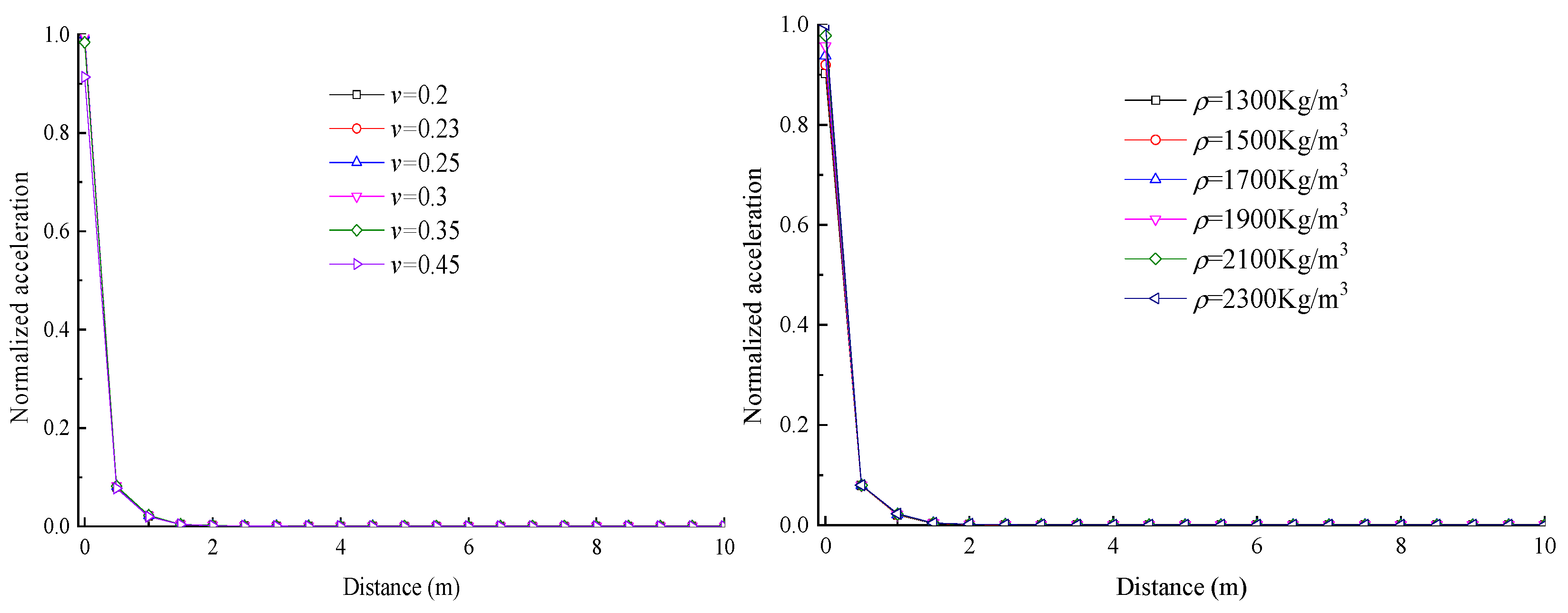
The heterogeneity of Young’s modulus and the train speed have enormous implications for the ground vibration, while Poisson’s ratio and the soil density have negligible effects.

(2)

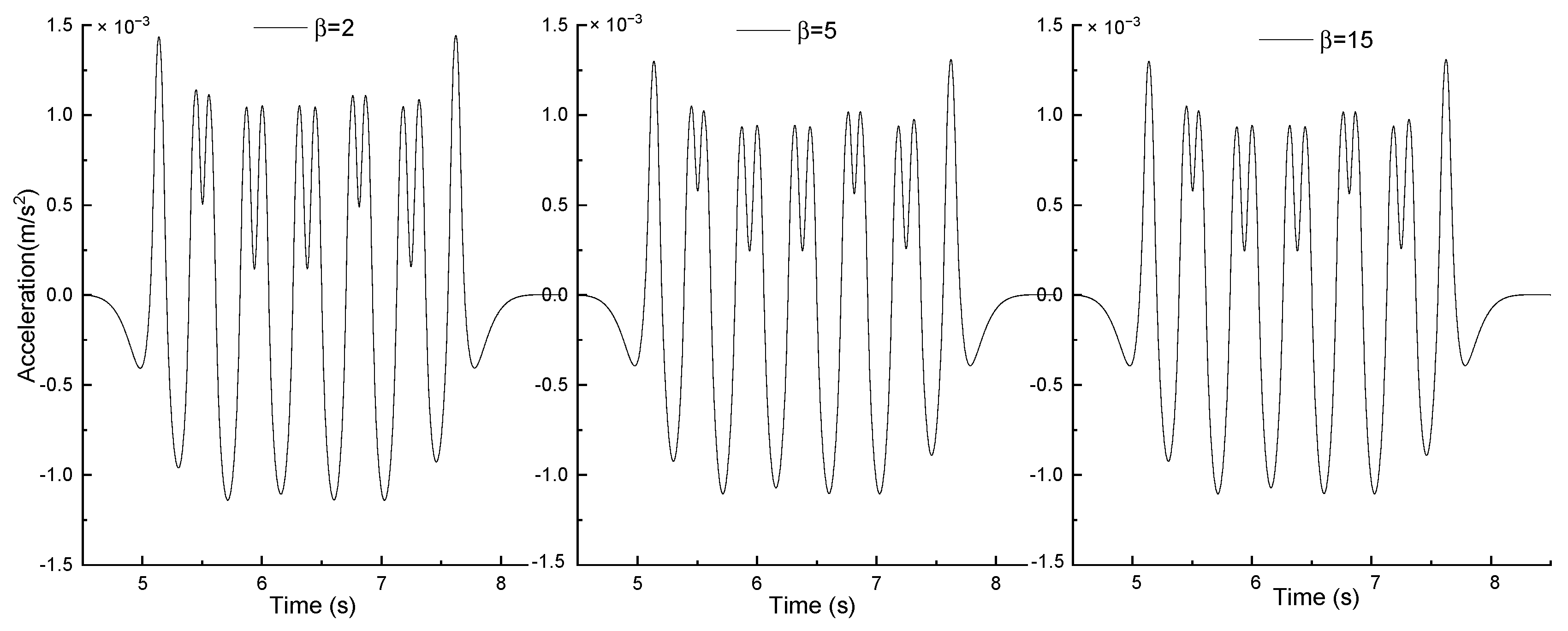
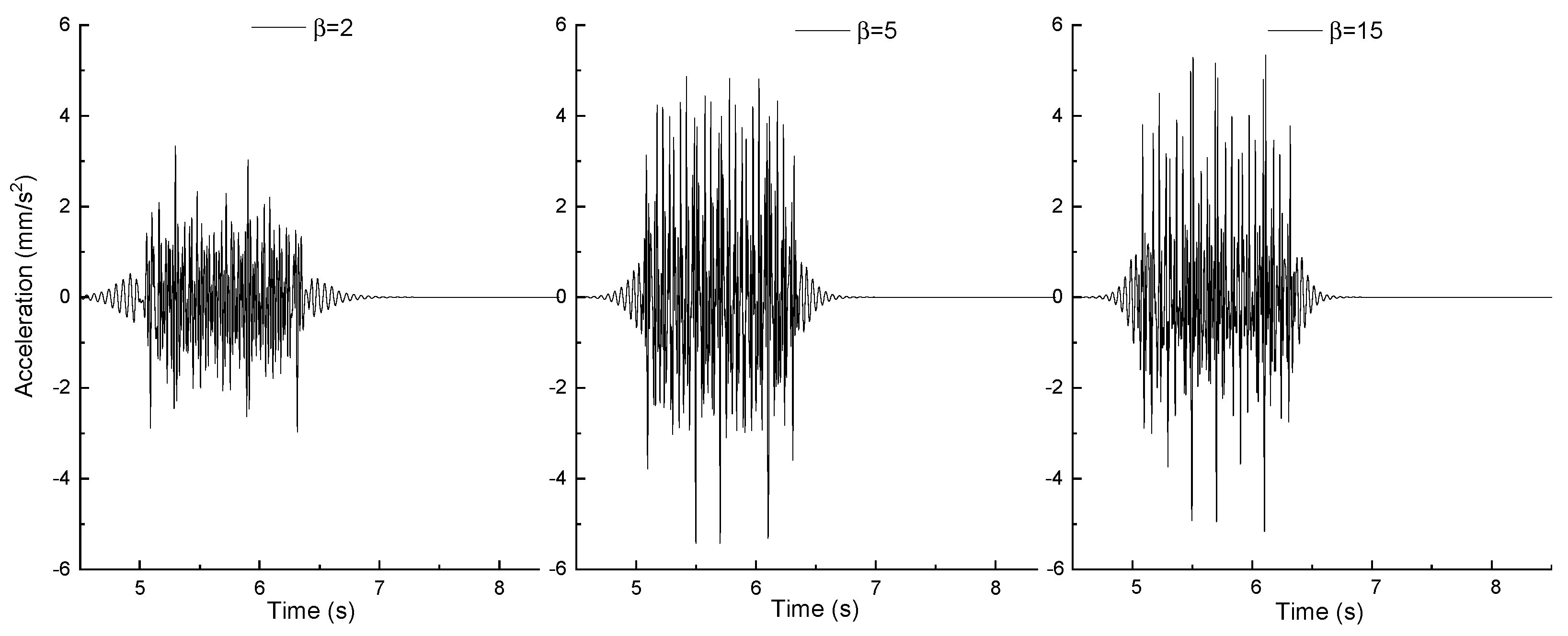
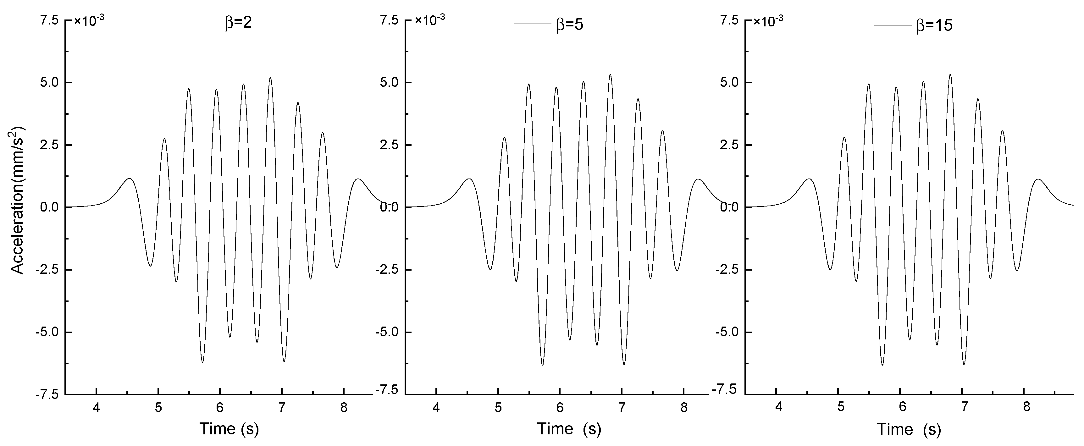
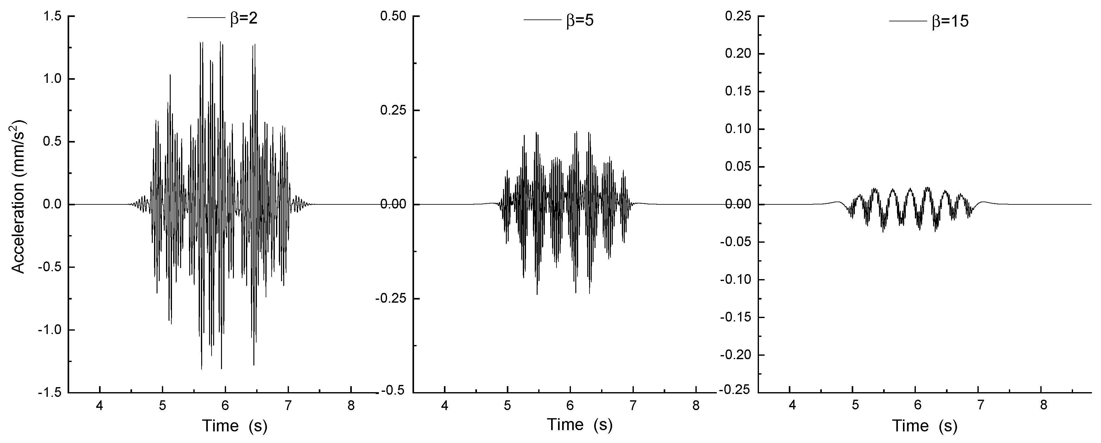
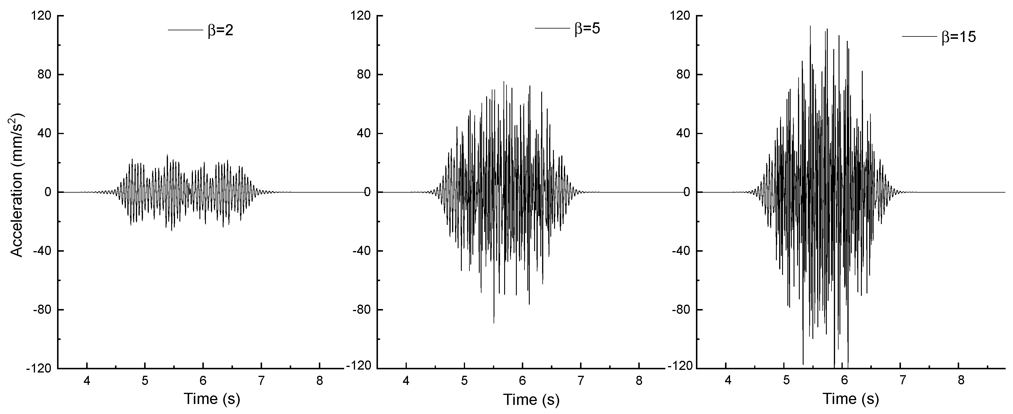
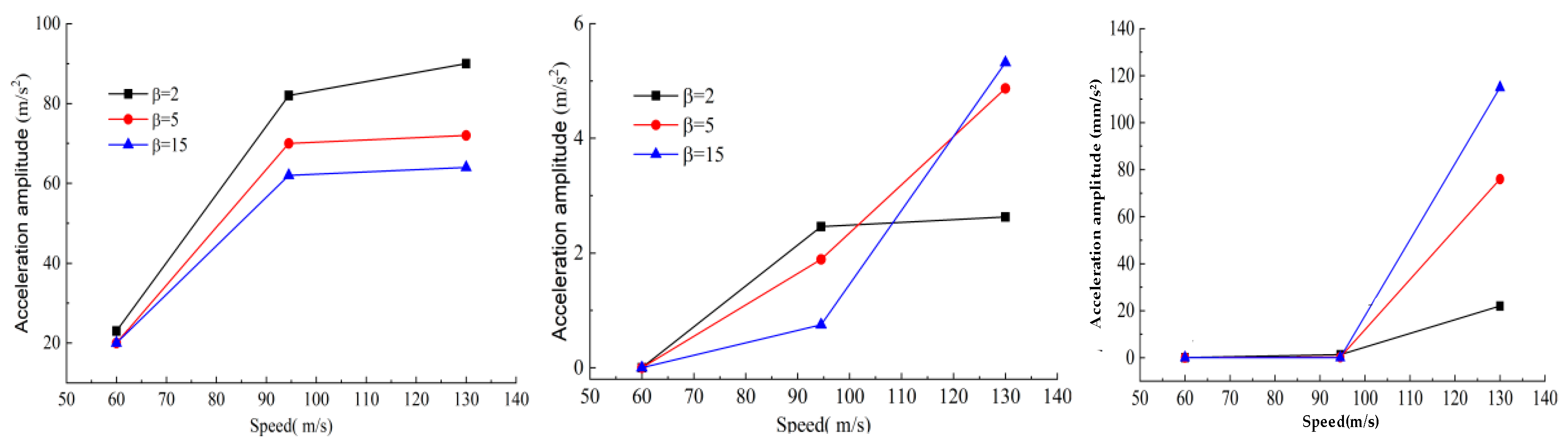
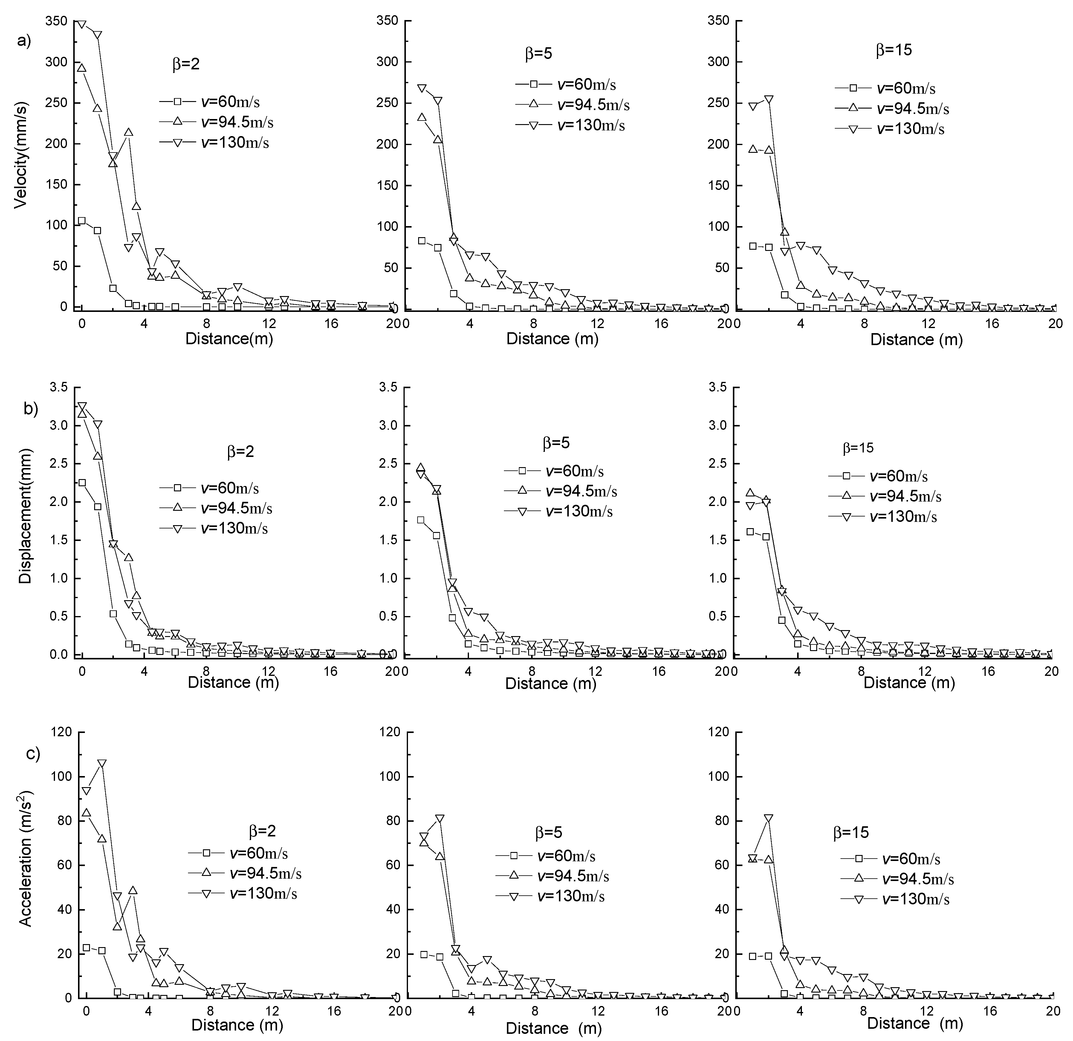
The upward acceleration is approximately equal to the downward one at a far distance from the track center. The superficial soil homogeneity significantly influences the ground vibration acceleration at 8 m and 28 m, and the impact pattern has a strong correlation with the train speed and the location. As the homogeneity coefficient increases, the peak acceleration continuously decreases in the transonic case, while it gradually increases in the supersonic case. To reduce the far-field acceleration, we can take measures to increase the soil homogeneity in the transonic case, while in the supersonic case, we should take steps to decrease the soil homogeneity.

(3)

The dominant frequency remains almost unchanged with varying β, while it shifts significantly with the train speed. The influence range of heterogeneity increases with increasing train speed. A local rebound in attenuation will occur in the supersonic case, and the maximum acceleration occurs at the outer edges of the track. The weak superficial soil can reduce the far-field acceleration level in the supersonic case.

The frequency–wave-number method proposed in this paper is an excellent model for dealing with the dynamic response of an elastic medium under a moving load, compared to the traditional 3D FEM. However, there are some other semi-numerical methods developed by scholars to avoid large computational storage based on their individual advantages [47]. Taking advantage of these methods gives us a new direction for improving the model in a future study. A random variable model incorporated into the frequency–wave-number method provides a perspective to consider soil heterogeneity; however, the non-uniformity of the ground soil is quite a complex problem in engineering practice and is not easy to describe accurately. The Weibull function used in this article makes it possible to easily take into account the foundation non-uniformity. For further investigation, it is a good idea to consider stochastic field theory [48] and some other distribution models proposed on the basis of in situ tests and back-analysis [49,50,51,52]. Furthermore, it can be found from Figure 15 that, for beta = 2, which indicates weaker ground homogeneity, ground acceleration has a limited increment when the train speed increases from 94.5 m/s to 130 m/s at an 8 m distance. This may be caused by the complex interrelationship between the train speed and soil wave velocity. A speed of 94.5 m/s is close to the shear wave velocity of the superficial soil. As the train speed increases to 130 m/s, the ground acceleration at 8 m increases significantly because of a high soil homogeneity level (beta = 5, 15). But when at a low soil homogeneity level (beta = 2), the uneven soil particles may cause a significant scatter of the surface wave, which reduces the vibration at an 8 m distance. However, it is regrettable that its clear intrinsic mechanism cannot be analyzed in this article, but this is also a direction of our future efforts.

References

1. Gao, G.Y.; Yao, S.F.; Sun, Y.M. Unsaturated ground vibration induced by high-speed train loads based on 2.5D finite element method. J. Tongji Univ. 2019, 47, 957–966. (In Chinese) [Google Scholar]
2. Beskou, N.D. Theodorakopoulos DD. Dynamic effects of moving loads on road pavements: A review. Soil. Dyn. Earthq. Eng. 2011, 31, 547–567. [Google Scholar] [CrossRef]
3. Barros, F.C.P.D.; Luco, J.E. Response of a layered viscoelastic half-space to a moving point load. Wave Motion 1994, 19, 189–210. [Google Scholar] [CrossRef]
4. Jin, B.; Yue, Z.Q.; Tham, L.G. Stresses and excess pore pressure induced in saturated poroelastic half space by moving line load. Soil. Dyn. Earthq. Eng. 2004, 24–42. [Google Scholar]
5. Chen, Y.; Beskou, N.D.; Qian, J. Dynamic response of an elastic plate on a cross-anisotropic poroelastic half-plane to a load moving on its surface. Soil. Dyn. Earthq. Eng. 2018, 107, 292–302. [Google Scholar] [CrossRef]
6. Cai, Y.Q.; Sun, H.L.; Xu, C.J. Steady state responses of poroelastic half-space soil medium to a moving rectangular load. Int. J. Solids Struct. 2007, 44, 7183–7196. [Google Scholar] [CrossRef]
7. Gao, G.Y.; Yao, S.F.; Yang, C.B. Ground vibration induced by moving train loads on unsaturated soil using 2.5D FEM. J. Harbin Inst. Technol. 2019, 51, 95–103. (In Chinese) [Google Scholar]
8. Eason, G. The stresses produced in a semi-infinite solid by a moving surface force. Int. J. Eng. Sci. 1965, 2, 581–609. [Google Scholar] [CrossRef]
9. Lu, Z.; Hu, Z.; Yao, H.L.; Liu, J.; Zhan, Y.X. An analytical method for evaluating highway embankment responses with consideration of dynamic wheel-pavement interactions. Soil. Dyn. Earthq. Eng. 2016, 83, 135–147. [Google Scholar] [CrossRef]
10. dos Santos, N.C.; Barbosa, J.; Calçada, R.; Delgado, R. Track-ground vibrations induced by railway traffic: Experimental validation of a 3D numerical model. Soil. Dyn. Earthq. Eng. 2017, 97, 324–344. [Google Scholar] [CrossRef]
11. Lefeuve-Mesgouez, G.; Mesgouez, A. Three-dimensional dynamic response of a porous multilayered ground under moving loads of various distributions. Adv. Eng. Softw. 2012, 46, 75–84. [Google Scholar] [CrossRef]
12. Dieterman, H.A.; Metrikine, A. Steady-state displacements of a beam on an elastic half-space due to a uniformly moving constant load. Eur. J. Mech. A/Solids 1997, 16, 295–306. [Google Scholar]
13. Sheng, X.; Jones, C.J.C.; Petyt, M. Ground vibration generated by a load moving along a railway track. J. Sound. Vib. 1999, 228, 129–156. [Google Scholar] [CrossRef]
14. Lefeuve-Mesgouez, G.; Le Houédec, D.; Peplow, A.T. Ground vibration in the vicinity of a high-speed moving harmonic strip load. J. Sound. Vib. 2000, 231, 1289–1309. [Google Scholar] [CrossRef]
15. Hwang, R.N.; Lysmer, J.J. Response of buried structures to traveling waves. J. Geotech. Eng. Div. 1981, 107, 183–200. [Google Scholar] [CrossRef]
16. Ba, Z.N.; Liu, Y.; Liang, J.W. Near-fault broadband seismograms synthesis in a stratified transversely isotropic half-space using a semi-analytical frequency-wavenumber method. Eng. Anal. Bound. Elem. 2023, 146, 1–16. [Google Scholar] [CrossRef]
17. Yang, Y.B.; Hung, H.H. A 2.5D finite/infinite element approach for modeling visco-elastic bodies subjected to moving loads. Int. J. Numer. Methods Eng. 2001, 51, 1317–1336. [Google Scholar] [CrossRef]
18. Yang, Y.B.; Hung, H.H.; Chang, D.W. Train-induced wave propagation in multi-layered soils using finite/infinite element simulation. Soil. Dyn. Earthq. Eng. 2003, 23, 263–278. [Google Scholar] [CrossRef]
19. Takemiya, H.; Bian, X.C. Substructure simulation of inhomogeneous track and layered ground dynamic interaction under train passage. J. Eng. Mech. Div. 2005, 131, 699–711. [Google Scholar] [CrossRef]
20. Bian, X.C.; Chen, Y.M.; Hu, T. Numerical simulation of high-speed train induced ground vibrations using 2.5D finite element approach. Sci. China Phys. Mech. Astron. 2008, 51, 632–650. [Google Scholar] [CrossRef]
21. Bian, X.C.; Jiang, H.; Chang, C.; Hu, J.; Chen, Y. Track and ground vibrations generated by high-speed train running on ballastless railway with excitation of vertical track irregularities. Soil. Dyn. Earthq. Eng. 2015, 76, 29–43. [Google Scholar] [CrossRef]
22. Gao, G.Y.; Yao, S.F.; Yang, J.; Chen, J. Investigating ground vibration induced by moving train loads on unsaturated ground using 2.5D FEM. Soil. Dyn. Earthq. Eng. 2019, 124, 72–85. [Google Scholar] [CrossRef]
23. Wang, R.; Hu, Z.P. Current situation and prospects of 2.5D finite element method for the analysis of dynamic response of railwaysubgrade. Rock. Soil. Mech. 2024, 45, 284–301. [Google Scholar]
24. Phoon, K.K.; Kulhawy, F.H. Evaluation of geotechnical property variability. Can. Geotech. J. 1999, 36, 625–639. [Google Scholar] [CrossRef]
25. Zhang, L.L. Reliability Theory of Geotechnical Engineering; Tongji University Press: Shanghai, China, 2011. (In Chinese) [Google Scholar]
26. Papadopoulos, M.; Francois, S.; Degrande, G.; Lombaert, G. The influence of uncertain local subsoil conditions on the response of buildings to ground vibration. J. Sound. Vib. 2018, 418, 200–220. [Google Scholar] [CrossRef]
27. Hu, H.; Huang, Y. PDEM-based stochastic seismic response analysis of sites with spatially variable soil properties. Soil. Dyn. Earthq. Eng. 2019, 125, 105736. [Google Scholar] [CrossRef]
28. Wang, Y.; He, J.; Shu, S.; Zhang, H.; Wu, Y. Seismic responses of rectangular tunnels in liquefiable soil considering spatial variability of soil properties. Soil. Dyn. Earthq. Eng. 2022, 162, 1074–1089. [Google Scholar] [CrossRef]
29. Alamanis, N.; Dakoulas, P. Effects of spatial variability of soil properties and ground motion characteristics on permanent displacements of slopes. Soil. Dyn. Earthq. Eng. 2022, 161, 1–22. [Google Scholar] [CrossRef]
30. Deng, E.; Liu, X.Y.; Ni, Y.-Q.; Wang, Y.-W.; Zhao, C.-Y. A coupling analysis method of foundation soil dynamic responses induced by metro train based on PDEM and stochastic field theory. Comput. Geotech. 2023, 154, 1051–1080. [Google Scholar] [CrossRef]
31. Wang, M.X.; Wu, Q.; Li, D.Q.; Du, W. Numerical-based seismic displacement hazard analysis for earth slopes considering spatially variable soils. Soil. Dyn. Earthq. Eng. 2023, 171, 1067–1079. [Google Scholar] [CrossRef]
32. Coelho, B.Z.; Nuttall, J.; Noordam, A.; Dijkstra, J. The impact of soil variability on uncertainty in predictions of induced vibrations. Soil. Dyn. Earthq. Eng. 2023, 169, 1055–1078. [Google Scholar]
33. Gao, G.Y.; Chen, G.Q.; Zhang, B. Analysis of active isolation of vertical non uniform fundamental wave barrier under train load. Vib. Shock. 2013, 32, 57–62. (In Chinese) [Google Scholar]
34. Zhou, F.X.; Cao, Y.C.; Zhao, W.G. Dynamic response of non-homogeneous foundation to rectangular moving loads. J. Lanzhou Univ. Technol. 2015, 41, 122–126. (In Chinese) [Google Scholar]
35. Zhou, F.X.; Cao, Y.C.; Zhao, W.G. Dynamic response analysis of non-uniform foundation under moving loads. Geotech. Mech. 2015, 36, 2027–2033. (In Chinese) [Google Scholar]
36. Ma, Q.; Zhou, F.X. Dynamic response of gradient non-uniform soil under moving loads. J. Nat. Disasters 2018, 27, 61–67. [Google Scholar]
37. Shi, L.W.; Ma, Q.; Shu, J.H. Dynamic responses of graded non-homogeneous unsaturated soils under a strip load. Chin. J. Theor. Appl. Mech. 2022, 54, 2008–2018. [Google Scholar]
38. Hou, H.; Yang, J.; Cheng, L. Simulation of Viscoelastic Artificial Boundary Based on Thin Layer Element. J. Yangtze River Sci. Res. Inst. 2020, 37, 164–169. (In Chinese) [Google Scholar]
39. Connolly, D.; Kouroussis, G.; Giannopoulos, A.; Verlinden, O.; Woodward, P.; Forde, M. Assessment of railway vibrations using an efficient scoping model. Soil. Dyn. Earthq. Eng. 2014, 58, 37–47. [Google Scholar] [CrossRef]
40. Feng, Q.S.; Cheng, G. Dynamic Characteristics Analysis of Ballastless Track Stiffness in Frequency Domain by Using Wavenumber Finite Element Method. J. China Railw. Soc. 2017, 39, 102–107. (In Chinese) [Google Scholar]
41. Deng, P.H.; Liu, Q.S.; Lu, H.F. FDEM numerical study on the mechanical characteristics and failure behavior of heterogeneous rock based on the Weibull distribution of mechanical parameters. Comput. Geotech. 2023, 154, 105–138. [Google Scholar] [CrossRef]
42. He, J.F. Analyses of Ground Dynamic Responses and Settlement by 2.5D FEM for Moving Train; Tongji University Press: Shanghai, China, 2010. (In Chinese) [Google Scholar]
43. Costa, P.A.; Colaço, A.; Calçada, R.; Cardoso, A.S. Critical speed of railway tracks: Detailed and simplified approaches. Transp. Geotech. 2015, 2, 30–46. [Google Scholar] [CrossRef]
44. Zhai, W.M.; Han, H.Y. Research on ground vibration caused by high-speed trains running on soft soil foundation lines. Sci. China Ser. E 2012, 42, 1148–1156. (In Chinese) [Google Scholar]
45. Yao, S.; Yue, L.; Xie, W.; Zheng, S.; Tang, S.; Liu, J.; Wang, W. Investigating the Influence of Non-Uniform Characteristics of Layered Foundation on Ground Vibration Using an Efficient 2.5D Random Finite Element Method. Mathematics 2024, 12, 1488. [Google Scholar] [CrossRef]
46. Liang, R.; Liu, W.; Ma, M.; Liu, W.N. An efficient model for predicting the train-induced ground-borne vibration and uncertainty quantification based on Bayesian neural network. J. Sound. Vib. 2020, 495, 908–922. [Google Scholar] [CrossRef]
47. Temimi, H.; Kurkcu, H. An accurate asymptotic approximation and precise numerical solution of highly sensitive Troesch’s problem. Appl. Math. Comput. 2014, 235, 253–260. [Google Scholar] [CrossRef]
48. Djehiche, B.; N’zi, M.; Owo, J.-M. Stochastic viscosity solutions for SPDEs with continuous coefficients. J. Math. Anal. Appl. 2011, 384, 63–69. [Google Scholar] [CrossRef]
49. Gao, G.Y.; Yao, S.F.; Sun, Y.M. 2.5D Finite Element analysis of unsaturated ground vibration induced by High Speed Rail Load. Earth-Quake Eng. Eng. Vib. 2019, 33, 234–245. [Google Scholar]
50. Gao, G.Y.; Yao, S.F.; Cui, Y.J. Zoning of confined aquifers inrush and quicksand in Shanghai region. Nat. Hazards 2018, 91, 1341–1363. [Google Scholar] [CrossRef]
51. Yao, S.F.; Zhang, Z.N.; Ge, X.R. Correlation between fracture energy and geometrical characteristic of mesostructure of marble. Rock. Soil. Mech. 2016, 37, 2341–2346. [Google Scholar]
52. Meng, Z.; Wang, Y.; Zheng, S.; Wang, X.; Liu, D.; Zhang, J.; Shao, Y. Abnormal monitoring data detection based on matrix manipulation and the cuckoo search algorithm. Mathematics 2024, 12, 1345. [Google Scholar] [CrossRef]
Figure 1. The finite element discretization of the foundation section under a vertical point force.
Mathematics 12 01750 g001
Figure 2. Verification of the proposed frequency–wave-number method for an elastic medium.
Mathematics 12 01750 g002
Figure 3. The attenuation and decay rate of the normalized ground displacement amplitude with distance in the x- and z-directions (Ugt = amplitude displacement at track center).
Mathematics 12 01750 g003
Figure 4. The effect of the soil parameters and velocity on the normalized acceleration attenuation.
Mathematics 12 01750 g004aMathematics 12 01750 g004b
Figure 5. Sensitivity analysis of the parameters to the normalized vibration amplitude.
Mathematics 12 01750 g005
Figure 6. The influence of the shape parameter m on the Weibull probability density function.
Mathematics 12 01750 g006
Figure 7. The normalized displacement results as the non-uniform soil model degenerates into a uniform one compared with the uniform soil [8].
Mathematics 12 01750 g007
Figure 8. A schematic diagram showing the interaction mechanism between the Euler track and non-uniform soil layers under the moving HST load.
Mathematics 12 01750 g008
Figure 9. Ground surface acceleration 8 m away from the moving HST load center in the subsonic case of 60 m/s.
Mathematics 12 01750 g009
Figure 10. Ground surface acceleration 8 m away from the moving HST load center in the transonic case of 94.5 m/s.
Mathematics 12 01750 g010
Figure 11. Ground surface acceleration 8 m away from the moving HST load center in the supersonic case of 130 m/s.
Mathematics 12 01750 g011
Figure 12. Ground surface acceleration 28 m away from the moving HST load center in the subsonic case of 60 m/s.
Mathematics 12 01750 g012
Figure 13. Ground surface acceleration 28 m away from the moving HST load center in the transonic case of 94.5 m/s.
Mathematics 12 01750 g013
Figure 14. Ground surface acceleration 28 m away from the moving HST load center in the supersonic case of 130 m/s.
Mathematics 12 01750 g014
Figure 15. Ground acceleration amplitude at 0 m, 8 m, and 28 m at different β and speeds.
Mathematics 12 01750 g015
Figure 16. Ground acceleration spectra at 0 m, 8 m, and 28 m at different β and train speeds: (a) 60 m/s; (b) 94.5 m/s; (c) 130 m/s.
Mathematics 12 01750 g016
Figure 17. Amplitude attenuation of ground vibrations at different train speeds with constant β: (a) velocity; (b) displacement; (c) acceleration.
Mathematics 12 01750 g017
Figure 18. Attenuation of acceleration level at different train speeds and β.
Mathematics 12 01750 g018