Mathematical Modeling for Robot 3D Laser Scanning in Complete Darkness Environments to Advance Pipeline Inspection

Abstract

This paper introduces an autonomous robot designed for in-pipe structural health monitoring of oil/gas pipelines. This system employs a 3D Optical Laser Scanning Technical Vision System (TVS) to continuously scan the internal surface of the pipeline. This paper elaborates on the mathematical methodology of 3D laser surface scanning based on dynamic triangulation. This paper presents the mathematical framework governing the combined kinematics of the Mobile Robot (MR) and TVS. It discusses the custom design of the MR, adjusting it to use of robustized mathematics, and incorporating a laser scanner produced using a 3D printer. Both experimental and theoretical approaches are utilized to illustrate the formation of point clouds during surface scanning. This paper details the application of the simple and robust mathematical algorithm RANSAC for the preliminary processing of the measured point clouds. Furthermore, it contributes two distinct and simplified criteria for detecting defects in pipelines, specifically tailored for computer processing. In conclusion, this paper assesses the effectiveness of the proposed mathematical and physical method through experimental tests conducted under varying light conditions.

1. Introduction

Currently, the hydrocarbon industry remains one of the principal supports of the country’s economy. Therefore, all the activities that are involved in this industry are worthy of the application of updated methods. Whether for gas or oil transportation, pipelines are the most effective way to achieve this task. All of the involved processes of transportation should be guaranteed to be optimal, aiming to avoid monetary losses or accidents. According to [1], most of the pipelines used in hydrocarbon transportation are under extreme conditions, such as temperature, pressure, corrosion, humidity, etc. These kinds of extreme conditions can lead to wear on the pipes. Currently, the most common material utilized for pipeline construction is carbon steel API 5L X65, X70, and X80. Nevertheless, some sewer and water transportation pipelines use concrete [2]. Although concrete and steel are durable materials, extreme weather conditions reduce their lifetime significantly. To prevent accidents and transportation delays in the pipeline, it is recommended to perform a periodic inspection. Therefore, pipeline inspection is one of the most important tasks for the industry. Normally, a complete inspection must detect various physical parameters whose values can be crucial for normal pipeline functioning. According to many years of tradition in this industrial branch, this kind of inspection is visual. The most natural way for its automation is the use of optical multi-sensing systems.

On the other hand, the authors of the present work have dedicated many years to 3D optical laser rotational scanning systems [3,4,5,6,7,8,9,10,11], and we have confirmed that our laser scanners, by default, naturally decrease their uncertainty, noise, and bias influence, and that their energetic losses and battery lifetime increase when operating in complete darkness. At the same time, in complete darkness, when traditional optical devices based on cameras of any type (APS, CMOS, CCD, omnidirectional fisheye, etc.) are almost unable to function, our optical system only increases its operational skills. Moreover, whereas the traditional optical inspection is applied on the external pipeline surface, our automated system is intended for internal application, which is more useful for specialists in structural maintenance, and it can localize more complex and hidden defects. These factors were the main inspiration for the present work.

In the national context of the authors, there are more than 17,000 km of pipelines around the Mexican national territory which are utilized for the transportation of hydrocarbons, according to PEMEX’s official site [12]. These pipelines differ in diameter depending on the branch type and purpose of the station. The vast majority of the principal branch diameter is no less than 24 inches (609 mm). The minimum and maximum diameters of said pipeline branches are 6 and 48 inches, respectively. Taking into account the international context, we analyze one of the largest pipelines around the globe, the Trans-Alaska Pipeline System, which is a pipeline system with about 800 miles (only in the main branch) of pipelines with a diameter of 48 inches (1022 mm) inches [13], and that, as mentioned before, is also under extreme cold weather conditions. These mentioned previously, pipeline systems represent only some of the places where the proposed system could be implemented. Taking into consideration all of the abovementioned factors, a research area was identified; hence, this following paper is presented. Since the abovementioned extreme conditions will also affect the tools utilized for inspections and the persons that perform such tasks, it is important to propose new methods or tools capable of realizing these tasks.

In the literature, some researchers have worked towards the automation and secureness of this task. There are autonomous applications for the inspection of either the internal or the external conditions of the pipelines [1]. In [14], the authors present a control scheme for an autonomous unmanned aerial vehicle (UAV) used for external inspection of a pipeline with the aid of image processing. Although the method allows for tracking the pipeline and performing measurements with cameras, it takes about 4 s to stabilize, making early data unreliable, in addition to occasionally tracking loss stabilization for periods of 1 s. Our system, however, performs reliable measurements from the first second to the end of the inspection. Introduced in [15] is the design and implementation of a robot with the autonomy for exploration of internal pipeline conditions that focusses on its capability to move inside it using wall-press caterpillars that drive the robot. By design, the robot presents limitations, since it is only suitable for reduced-diameter dimensions pipelines, specifically 150 mm. In a complex pipeline system, it could be possible that the diameter varies within sections, preventing the completion of the inspection. Moreover, the caterpillar tension against the pipeline’s wall must be manually adjusted to any environment conditions, which traduces into setting/calibration time needed to start the inspection process. To be able to move with enough velocity along the pipeline, the caterpillar should have enough torque, which can traduce on energy loss due to the high number of DC motors functioning. The inspection system uses cameras, and therefore it needs a light source to perform well. The system needs to be operated remotely. The authors in [16] made a review of the different hybrid robots that seize the advantage of two locomotion systems to become robust and flexible in terms of application necessity. Many of them face similar restrictions and difficulties in performing objective tasks. As a main disadvantage, none of these robots with the abovementioned motion system has the ability to travel or inspect from bigger- to smaller-diameter pipes. According to [16], one of the main problems of the in-pipe inspection robots is that it supposes the inability to navigate with confidence along the pipeline branches. Reference [17] uses stereo vision to detect defects. Onboard cameras require a robot lightning system, as without it, the mapping quality decreases. Having to process images from three cameras is time consuming due to the high quantity of data that each camera provides. In addition, a large quantity of acquired information becomes irrelevant when searching for laser profiling on the author’s chosen application. The relation between camera’s pixel resolution and laser thickness creates the necessity to find the midpoint of the laser ray projected onto the surface to precisely locate the center of the circular section of the pipeline. In [15], the mobile robot is autonomous and can travel along the pipeline, provided that it integrates some different sensing elements, which each add different capabilities each. This results in several extra sensor elements, if it is required to have a fully autonomous device. Presented in [18] is a review of the monitoring techniques for pipelines. Among the most popular visual techniques currently are those that use a Closed-Circuit Television (CCT) or a laser scanner. Nevertheless, execution time, memory requirement, and energy cost for the detection methods are still important aspects to be improved. Laser Scanner data are normally distorted by distance, laser-emitting wavelength, and incidence angles. Even though there are some methods aiming to decrease this level of distortion [19], this adds complex comparisons that increase processing time.

As background for this paper, it is relevant to notice that, previously, the authors proposed an original system for structural health monitoring [20]. It was observed in many cases that its main weak point is its significant sensitivity to ambient light noise and, correspondingly, higher measurement uncertainty due to this factor. This was a main reason to search an application where our original patented 3D laser scanner [21] can enhance its performance. Pipeline inspection was a good candidate for this, and during the experimentation with the most recent prototype inside a pipeline model, some other significant advantages of our method were discovered. Those advantages are the focus of the main novelty and contribution of the herein presented work. Thus, a novel scanning algorithm for the Technical Vision System (TVS) is presented in this paper, and is used to scan the internal condition of a pipeline. This TVS enables a robotic mechanism to perform a detailed surface inspection of a pipe’s internal surface, being able to identify obstructions, perforations, or weariness in the physical structure. Some of the system’s advantages are listed herein. The scanning system is capable of path planning, defect identification, defect mapping, and data storage. In addition, having similar dimensions to the robot in [15], the proposed system is suitable for a wider range of pipeline diameters, ranging from 220 mm up to 1022 mm. The system performed better in dark environments without an external or onboard extra lighting system such as the ones in [14,17,18]. Unlike [17], the TVS signals, by nature, outstrip the necessity of a preprocessing stage to find the laser ray. The scanning methodology decreases the effects mentioned in [17,19] by constringing spatial positioning, helping to maintain optimal physical conditions for the laser propagation in the optical channel.

The main reason for this paper was to find, among different possible approaches, a mathematical formalism that optimizes the system’s data acquisition in the identification of the physical characteristics of the pipe’s surface, either by reducing the calculation time or by avoiding the necessity of redundant information flow to secure the system’s reliability.

This paper is organized into following sections. After the Introduction, the second section presents the theoretical concepts of the scanning system; it describes the details of the design and electromechanical aspects, as well as the application requirements for the specific task: pipeline inspection. The sections afterward present the scanning methodology developed to acquire precise point clouds on the specific physical conditions for pipe evaluation, and afterward, the experimentation made to validate the scanning method, as well as the mathematic approach used for the identification of defects by point cloud segmentation, and corresponding results. Finally, discussions and conclusions provide closure to the presented paper.

2. Materials and Methods/Theoretical Concepts

The laser scanner introduced in [3,4] bases its functionality on the reflection directed laser ray into an object. The TVS has been widely used in researchers’ work. Numerous experiments confirm the system’s precision improves when isolating it from non-laser light sources. Illuminated environments, like daylight outdoors, yield unstable signals with low signal-to-noise ratios (SNR), leading to measurement errors. Instead, dark environments produce high SNR signals, enhancing precision. This isolation, typically a drawback, proves to be advantageous for in-pipe inspection, ensuring higher signal quality by eliminating external light interference. Internal darkness optimally propagates signals, enabling precise scanner operation.

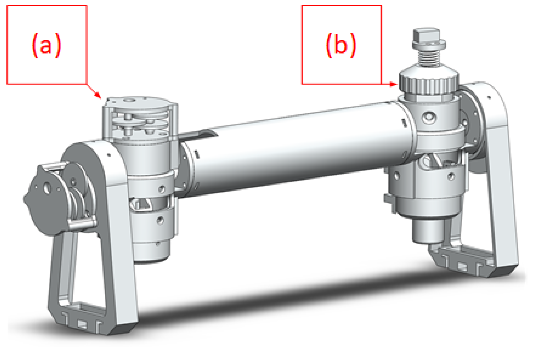
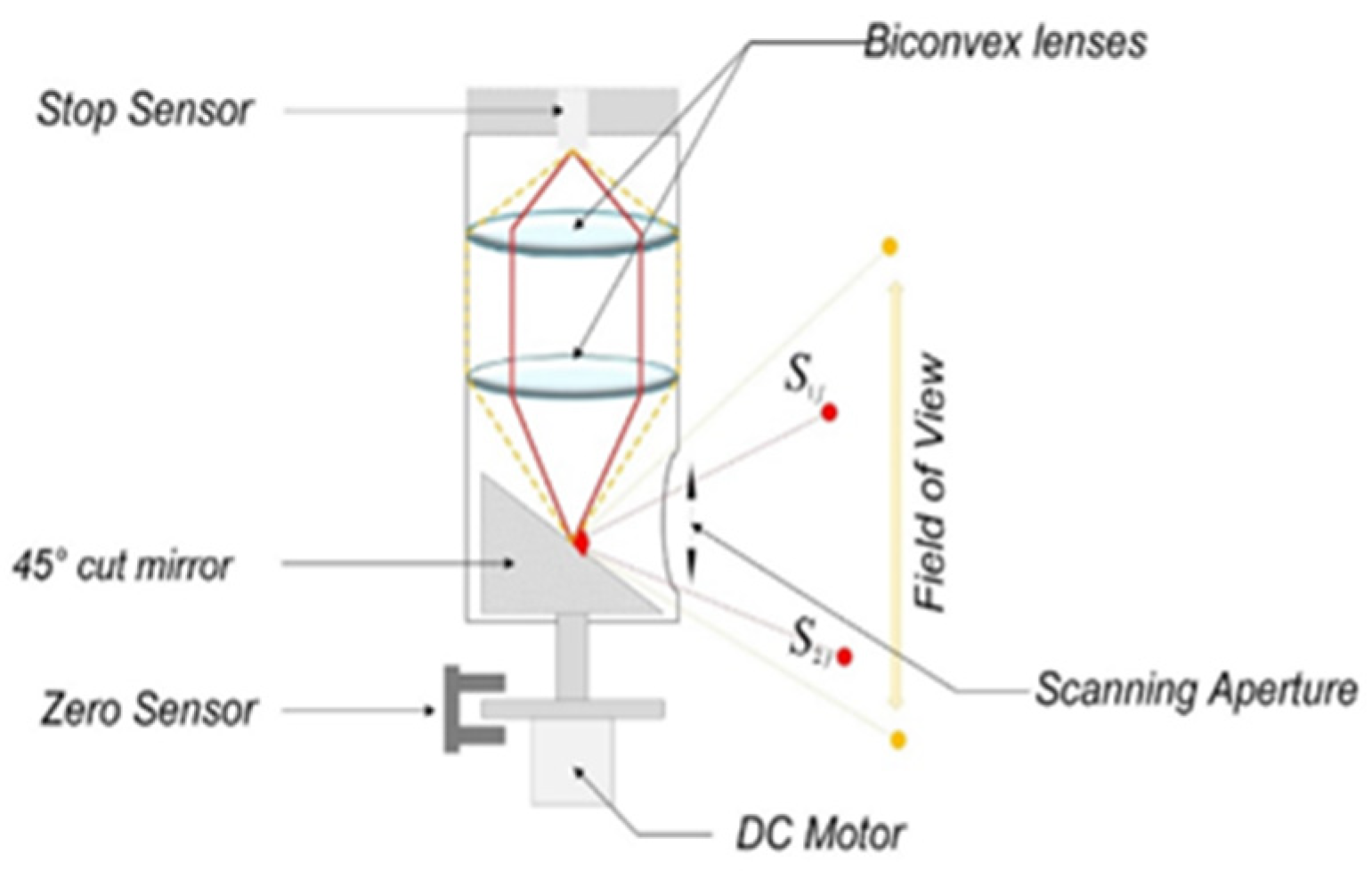
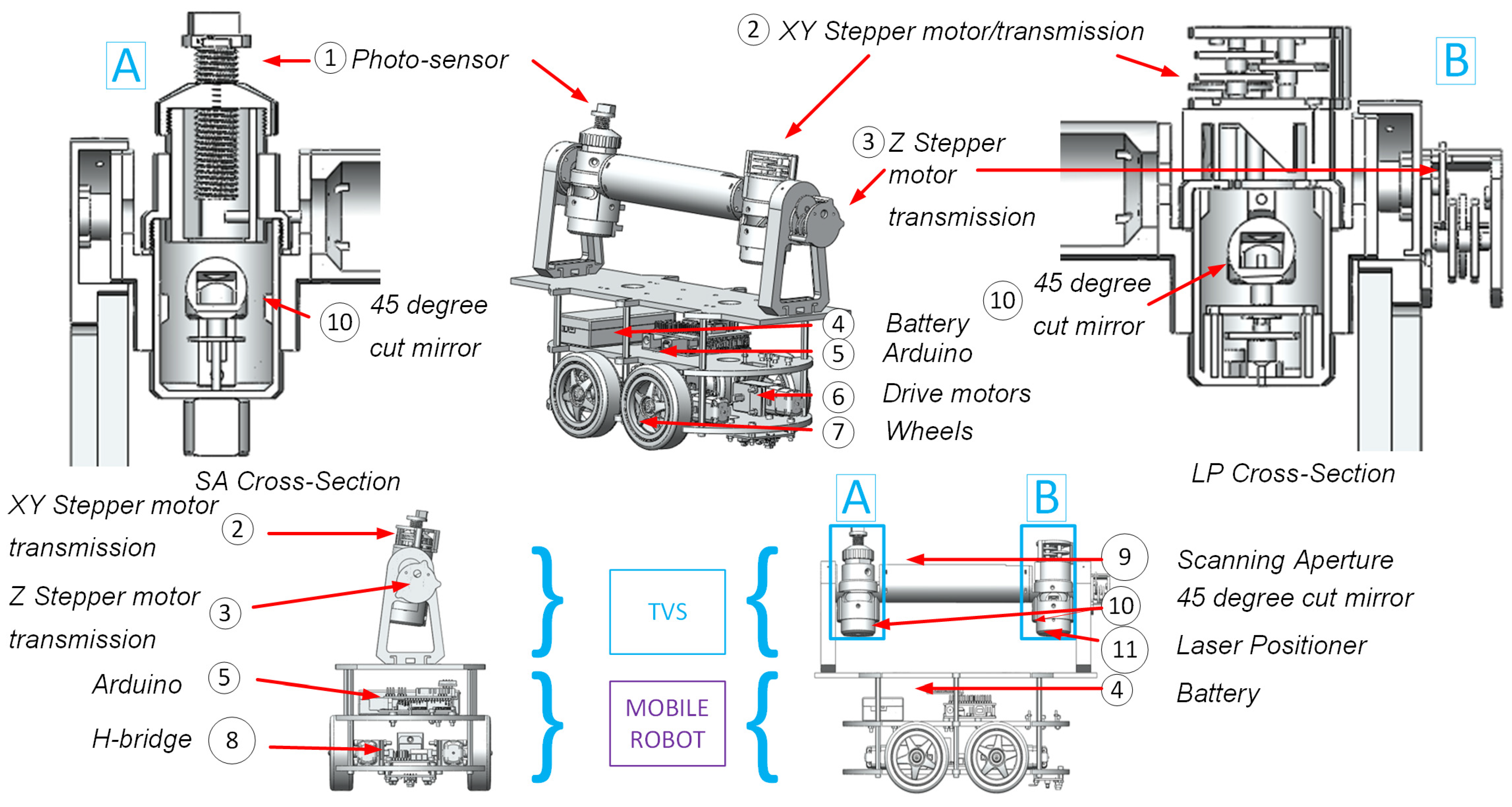
2.1. Scanning System

The Optical Laser Scanner or TVS is the principal sensing element used for measurements in the inspection system (see Figure 1).

The TVS consists of two principal nodes: a laser source, which is the active one, and an electro-optical sensing element, which is the passive one. The laser source uses a red laser in the 633 nm wavelength directed towards a region of interest using step DC motors and a set of 45°-cut mirrors and biconvex lenses. This mechanism is called a Laser Positioner (LP) (Figure 1a). As mentioned, the LP has two step-motors each for individual horizontal and vertical movement. The step motors have 20 steps per revolution and an attached gear box with a 1:256 ratio for horizontal/vertical movement, with a voltage level of 5 V and max current of 250 mA. The LP provides the TVS with the ability to move, and highlights any point in space with the known angles ${\alpha }_{ij},{\gamma }_{ij}$. The Scanning Aperture (SA) is the sensing node, and it has a 45°-cut mirror that rotate constantly, driven by a DC motor that can meet up to 17,000 revolutions per minute (rpm) (Figure 1b). It receives and redirects the reflected energy of the laser from the object’s surface and focuses it with two biconvex lenses to a stop sensor, which is a BPW77NB phototransistor sensible to visible and near-infrared radiation (480 to 1080 nm bandwidth) with fast response times (turn on/off time between 5–6 μs). An optocoupler (called a zero sensor) used in the base of the mirror keeps track of the rotation and provides a signal. With the signal from the optocoupler (rotation) and the phototransistor (laser-reflected energy) compared to a reference (clock), it is possible to calculate the ${\beta }_{ij}$ reflection angle. A detailed diagram of the SA is shown in Figure 2. With the angles ${\alpha }_{ij},{\gamma }_{ij},{\beta }_{ij}$ and a known separation between the two elements, the 3D spatial coordinates of the object’s reflection point can be calculated using the Law of Sines. This theory is called dynamic triangulation, and it is represented from its top view in Figure 3. The detailed construction and principles of the laser scanner with theoretical concepts are given in [3,4]. The electronic, mechanical, and design features of the TVS create limitations to the free movement of the elements, restricting the Field of View (FOV). Even though the TVS FOV is not 360 spatial degrees, it is enough to perform spatial measurements with the scanner, as has been widely demonstrated through several research works [3,4,5,6,7,22].

Although this paper analyses the methodology for precise pipeline inspection with our patented TVS [21], any type of robotic mechanism or mobile robot could be adapted to work with our scanning system. Nevertheless, to experimentally demonstrate the functionality of our inspection method, a mobile robot was selected. The Smart V2.0 mobile robot is commonly utilized for autonomous navigation tasks in the literature [23,24,25,26]. Researchers demonstrate its suitability for inspection, despite being designed for didactic purposes. Our research team significantly redesigned the standard Smart V2.0, incorporating our patented TVS prototype atop it using 3D printing. In total, about 85% of the details of the original robot were totally replaced by our original new design printed on a 3D printer, with additional enforcement of the mechanical strength. This modification lowers the center of mass and enhances the precision of the wheel drives for improved dead reckoning with our special control algorithm. Figure 4 consists of two subsystems: the Laser Scanner (TVS) and the Mobile Robot (MR). The TVS is mounted onto the MR, enabling it to travel along pipeline branches. This design provided for the application, the scanning methodology, aims to optimize the collaborative work of the robot and the TVS, strengthening the system’s autonomous navigation properties due to the scanner’s capability for adjustable obstacle detection.

Due to the TVS’s enhanced performance in dark environments (demonstrated in the “Experimental Evaluation” Section), the system does not require an onboard illumination tool. Nevertheless, if necessary, an illumination tool or flashlight system can be added to the robotic design, such as the one presented in [17]. The fact that there is no necessity for a light source is beneficial in energy savings, in comparison to other systems used for internal pipeline inspection, such as those mentioned in [17,27]. The power consumption to the autonomous robot that extra illumination could represent, however minimal, becomes significant in long inspection periods. The fact that the system avoids the necessity for such a tool means that this feature’s power consumption is zero. The MR has 6.5 cm diameter wheels, and can carry up to 2 kg, allowing the inspection system to travel along the pipe even if there are contaminant elements on the surface such as water, oil, and other fluids transported by pipelines.

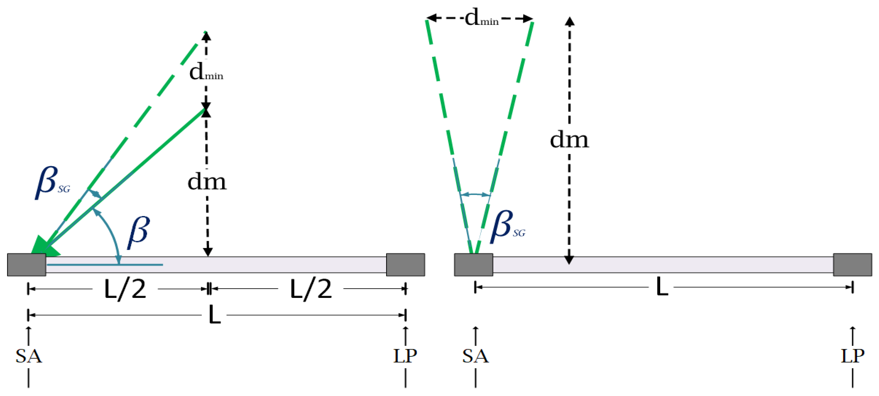
2.2. Mechanical Analysis and Kinematics Modeling

The following section describes the algorithms and mathematics aspects of the proposed pipeline scanning method. Our proposal performs the measurements of the environment dimensions using the laser source. It only requires the initialization (save into the MR memory the initial spatial coordinates of the start point and the initial values of roll-pitch-yaw-angles at this moment). The changing conditions of the mobile robot, position, and wheel slippage are compensated by the homogeneous transformation matrix, and can be sensed using an accelerometric platform [28]. The datasets measured using the TVS are then post-processed to evaluate the physical condition of the pipeline by comparison between the pipeline’s actual measured conditions and the manufacturing specifications of the pipeline’s blueprints. Defects are highlighted to make a second scan, and therefore (with the acquired information) are able to make decisions on the required maintenance.

2.2.1. Mechanical Analysis

Represented by equation system (1) is the MR’s movement.

$$\begin{array}{l}{\dot{x}}_{MR}(t)=v_{MR}(t)\cos ({\theta }_{MR}(t))\\ {\dot{y}}_{MR}(t)=v_{MR}(t)\sin ({\theta }_{MR}(t))\\ {\dot{\theta }}_{MR}(t)={\omega }_{MR}(t)\end{array}$$

(1)

In the system of equations, ${\dot{x}}_{MR}(t)$, ${\dot{y}}_{MR}(t)$ are the Cartesian coordinates of the MR on the moving plane. ${\dot{\theta }}_{MR}(t)$ is the angle between the x-axis of the Universal Cartesian Coordinate System (moving plane $CC{S}_1$) and the MR’s movement propagation line. ${\omega }_{MR}(t)$ is the angular velocity of the MR’s wheels, and $v_{MR}(t)$ is the MR’s linear displacement velocity, which is parallel to the x-axis of the Inertial Reference System 2 ($IR{S}_2$). Figure 5 depicts these variables in a simulated inspection environment. The control signals for the inspection system are obtained with the system of Equation (1) and the dynamic triangulation mathematics. To achieve this, the following condition should be presented. The operation velocities (2) of the inspection system are obtained with (1).

$${\omega }_{SA}>>{\omega }_{SV}>>{\omega }_{MR}$$

(2)

Equation (2) is the relation that should satisfy to assure the correct functioning of the inspection system. There, ${\omega }_{SA}$ is the SA rotation velocity, ${\omega }_{SV}$ is the scanning velocity of the PL, and ${\omega }_{MR}$ remains as MR’s wheels movement velocity. The SA rotation velocity ${\omega }_{SA}$ is related to the data-acquisition capability of the TVS under condition (3), as follows:

$$S_{r\#}=\frac{F_T}{{\omega }_{SA}/60}$$

(3)

Here, $S_{r\#}$ is the number of standard pulses with a sampling frequency, $F_T$, during one complete rotation of scanning aperture mirror, acquired by the Teensy in one complete SA rotation at a constant rotation velocity. From this, it is possible to determine the smallest graduation, ${\beta }_{SG}$, or the resolution of the ${\beta }_{ij}$ angle measurement. It is determined by (4) the following:

$${\beta }_{SG}=\frac{360}{S_{\#R}}$$

(4)

In contrast to [20], where the ${\beta }_{SG}$ is fixed, in the present application, the TVS supposes a slight margin to adjust ${\beta }_{SG}$ for rough/detailed scanning. Knowing the resolution, the total time it takes the system to make a single-point measurement is important to operation times. This is calculated by Equation (5).

$$m_{tt}=(k)(m_t)+p_t$$

(5)

where $m_{tt}$ is the total measurement time, $k$ is the number of points taken to make the measurement (usually providing three coordinates, averaging in each of the k scanned points in Figure 5), $m_t$ is the time that takes the SA to reach $k$ complete rotations, and $p_t$ is the processing time constant, which is normally 7 ms. $m_{tt}$ can be used to determine the MR’s change in position once the TVS has finished measuring one point with its 3D coordinates. If the MR’s position is changed by a difference bigger than $d_{SG}({\beta }_{SG})$, the measurement should not be considered reliable. Equations (6) and (7) describe this.

$${[{\dot{x}}_{MR}(m_{tt})]}_2-{[{\dot{x}}_{MR}(m_{tt})]}_1\le d_{SG}({\beta }_{SG})$$

(6)

$$d_{SG}({\beta }_{SG})=d_m\tan ({\beta }_{SG})$$

(7)

where $d_{SG}({\beta }_{SG})$ is the minimum distance change that the TVS will be capable to measure, and ${\dot{x}}_{MR}(m_{tt})$ 1 and 2 represent the final and initial positions, respectively, of the MR in the $x$ axis of the inertial Cartesian system, and $d_m$ is the distance from the center of TVS to the measured surface.

With (2)–(6), we can obtain the equation system that defines the inspection device operation.

$$\begin{array}{c}{[v_{MR}(m_{tt})\cos ({\omega }_{MR}(m_{tt}))]}_2-{[v_{MR}(m_{tt})\cos ({\omega }_{MR}(m_{tt}))]}_1\le d({\beta }_{SG})\\ {[v_{MR}(m_{tt})\cos ({\omega }_{MR}(m_{tt}))]}_2-{[v_{MR}(m_{tt})\cos ({\omega }_{MR}(m_{tt}))]}_1\le d_m\tan (\frac{360}{S_{\#R}})\\ {[v_{MR}(m_{tt})\cos ({\omega }_{MR}(m_{tt}))]}_2-{[v_{MR}(m_{tt})\cos ({\omega }_{MR}(m_{tt}))]}_1\le d_m\tan (\frac{360{\omega }_{SA}}{60F_T})\\ {[v_{MR}(m_{tt})\cos ({\omega }_{MR}(m_{tt}))]}_2-{[v_{MR}(m_{tt})\cos ({\omega }_{MR}(m_{tt}))]}_1\le d_m\tan (6\frac{{\omega }_{SA}}{F_T})\\ {[r_{MRW}{\omega }_{MR}(m_{tt})\cos ({\omega }_{MR}(m_{tt}))]}_2-{[r_{MRW}{\omega }_{MR}(m_{tt})\cos ({\omega }_{MR}(m_{tt}))]}_1\le d_m\tan (6\frac{{\omega }_{SA}}{F_T})\end{array}$$

(8)

Using (5) on (8), Equation (9) is the one that relates the restrictions for the velocities of ${\omega }_{SA}$, ${\omega }_{MR}(t)$, and ${\omega }_{SV}$.

$$\begin{array}{c}{[r_{MRW}{\omega }_{MR}((k)m_t+p_t)\cos ({\omega }_{MR}((k)m_t+p_t))]}_2-[{[r_{MRW}{\omega }_{MR}((k)m_t+p_t)\cos ({\omega }_{MR}((k)m_t+p_t))]}_1\le d_m\tan (6\frac{{\omega }_{SA}}{F_T})\\ {[r_{MRW}{\omega }_{MR}\left((k)\frac{{\omega }_{SA}}{60}+p_t\right)\cos \left((k)\frac{{\omega }_{SA}}{60}+p_t\right)]}_2-[r_{MRW}{\omega }_{MR}\left((k)\frac{{\omega }_{SA}}{60}+p_t\right)\cos {({\omega }_{MR}\left((k)\frac{{\omega }_{SA}}{60}+p_t\right)]}_1\le d_m\tan (6\frac{{\omega }_{SA}}{F_T})\end{array}$$

(9)

Equation (9) is defined by constants $r_{MRW}$, $p_t$, $k$, $m_t$, and $F_T$, and from there, velocities ${\omega }_{SA}$, ${\omega }_{MR}$, and ${\omega }_{SV}$ can be related. Equations (2) and (8) are conditional parameters for the pipeline inspection with the TVS. In (10), the minimal resolution of one axis measurement, $d_{SGx}$, is a constraint parameter for the measurement precision, due to the restriction of $k$, given the velocities ${\omega }_{SA}$ and ${\omega }_{MR}$. That is, the smaller the relationship between the two velocities, the fewer $k$ points the system is capable of measuring and averaging, which traduce in an increment of measurement uncertainty.

$$\begin{array}{c}{v}_{MR}((k)\frac{{\omega }_{SA}}{60}+p_t)\cos ({\omega }_{MR}((k)\frac{{\omega }_{SA}}{60}+p_t))\le d_m\tan \left(6\frac{{\omega }_{SA}}{F_T}\right)\\ r_{MRW}{\omega }_{MR}.\cos ({\omega }_{MR}((k)\frac{{\omega }_{SA}}{60}+p_t))\le d_m\tan \left(6\frac{{\omega }_{SA}}{F_T}\right)\\ {\dot{x}}_{MR}(m_{tt})\le d_{SGx}({\beta }_{SG})\end{array}$$

(10)

Then, Equation (11) could be the restriction parameter to defect localization (depending on MR orientation within $CC{S}_1$ in Figure 5).

$${\dot{y}}_{MR}(m_{tt})\le d_{SGy}({\beta }_{SG})$$

(11)

Figure 6 represents the minimal linear displacement resolution, $d_{SGy}$, which defines the minimum depth variation for the TVS to perceive. This means that the smaller $d_{SGy}$ is, the more detailed a defect that could be encountered by the inspection system is. Therefore, the value is classified according to

Table 1. Failure classification by depth/dimensions.

Failure	Defect Location	Code	Dimensions
Corrosion	Internal	1	0.2–0.8 mm
Weld Failure	Internal	2	10 mm
Perforation	Internal/External	3	-
Crack	Internal/External	4	10–30 mm
Manufacturing Defects	Internal	5	10–100 mm
Deformation	Internal/External	6	>20 mm

. The Table enlists the characteristic dimensions of different typical pipes failures, according to [2,29,30]. Also, the location and code given by our algorithm in the identification process is provided.

The system identifies defects throughout the inspection process. Shown in Figure 7 is the representation of how the corrosion failure dimension is supposed to be detected. Within a pipe’s surface, the algorithm looks into the position vector’s magnitudes for differences around 0.2–0.8 mm label as a typical size of corrosion cavity. Equation (12) is the difference between the magnitude of position vector (from circle center), ${\overrightarrow{P}}_{ij}$, and position vector, ${\overrightarrow{P}}_{ij+1}$.

$$\begin{array}{l}dif{f}_{pij/pij+1}=\left|{\overrightarrow{P}}_{ij}\right|-\left|{\overrightarrow{P}}_{ij+1}\right|\\ cfd=clu>dif{f}_{pij/pij+1}>cll\\ cfd=0.8>dif{f}_{pij/pij+1}>0.2\end{array}$$

(12)

where $cfd$ is the corrosion failure detection, $dif{f}_{pij/pij+1}$ is the surface depth difference, $cll,clu$ are the lower cavity bound and upper cavity bound, respectively, and ${\overrightarrow{P}}_{ij},{\overrightarrow{P}}_{ij+1}$ are the $ij$ th consecutive measured points being compared.

Weld failure and manufacturing defects are identified once the point cloud presents a uniform center or diameter change, and it is presented in (13). If the diameter change is within weld failure dimension and returns to the original state after MR movement, it is classified as a weld failure. If the center of the point cloud of the pipe changes its position, it is classified as a manufacturing defect.

$$\begin{array}{l}{C}_{pij/pij+1}\to C_{pij}=C_{pij+1}\\ D_{pij/pij+1}\to D_{pij}-(D_{pij+1}+D_{\lim })=0\end{array}$$

(13)

where $C_{pij/pij+1}$ is the position change of the pipeline circumference center, $D_{pij/pij+1}$ is the pipeline’s diameter change, and $D_{\lim }$ is the diameter change limit.

Deformation is classified using the RANSAC algorithm. Finally, in the event of a perforation, the algorithm classifies the defect using the external light presence.

Depending on the inspection priority, the TVS can be set to classify defects with smaller dimensions (code 3-1 on Table 1), and the velocities ${\omega }_{SA}$ and ${\omega }_{MR}$ and the value of $k$ are the variables that indicate the required precision.

$$d_{SGy}=\frac{\sqrt{{d_m}^2+L/2^2}\sin ({\beta }_{SG})}{\sin (180-{\beta }_{SG}-(90+{\tan }^{-1}(\frac{d_m}{L/2}))}$$

(14)

With the mentioned constraint parameters of $d_{SGy}$ in (14), the system operation velocities ${\omega }_{SA}$, ${\omega }_{SV}$, and ${\omega }_{MR}$ of the MR are selected using algorithm logic and classification dimensions, where constraints are set using specific inspection requirements and control velocities stated, according to Table 1.

After parameter restriction using the application requirements, the TVS measurements are adjusted to the point cloud with the MR movement equations, as seen in (15).

$$Tv=\left[\begin{array}{c}{\dot{x}}_{MR}(t)\\ {\dot{y}}_{MR}(t)\\ {\dot{\theta }}_{MR}(t)\end{array}\right],S{S}_{ij}=\left[x_{ij},y_{ij},z_{ij}\right]$$

(15)

where $S{S}_{ij}$ is the point cloud result of the surface scan of $i*j$ scanned points (mesh in Figure 5), which is spatially translated with the translation vector, $T_v$, defining the current position of the MR along its physical trajectory. The current position of the MR is known at this moment by several simultaneous registers, such as: simple count of averaged wheels revolutions; the double integral of accelerometer measurements; and, finally, counting the system internal time of functioning, which indirectly permits us to estimate a current MR displacement. The averaging of these three different physical estimation methods for the same coordinate permits us to decrease its uncertainty until it becomes a negligible value, thanks to the implemented multiparametric approach.

2.2.2. Kinematics Modeling/Orientation Detection

As mentioned above, the TVS knows its spatial orientation with the aid of a gyroscope/accelerometric platform. Then, after point clouds are scanned, some mathematical adjustment should be conducted to link/joint the clouds of the measured points with three-dimensional coordinates. This adjustment is performed with the homogeneous transformation matrix of translation and rotation. The homogeneous transformation matrix, $T$, represented in (16), is the matrix of 4 by 4 elements that contains the transformation of a vector or point from a coordinated system to another. Its components are the rotation matrix, the translation vector, the perspective transform, and the scale relation, respectively.

$$T=\left(\begin{array}{cc}{R}_{3x3}& p_{3x1}\\ f_{1x3}& w_{1x1}\end{array}\right)=\left(\begin{array}{cc}Rotation& Traslation\\ Perspective& Scale\end{array}\right)$$

(16)

The rotation matrix on the $\widehat{z}$ axis by an angle $\theta$ is Equation (17), in this scenario; the angle $\theta$ is the same as the MR inclination angle with respect to the moving plane ${\dot{\theta }}_{MR}(t)$.

$$R(z,\theta )=\left[\begin{array}{ccc}\cos \theta & -\sin \theta & 0\\ \sin \theta & \cos \theta & 0\\ 0& 0& 1\end{array}\right]$$

(17)

When comparing a static reference system $O_{xyz}$ ($CC{S}_1$ in Figure 5) to the rotated ${O^{\prime }}_{x^{\prime }{y}^{\prime }{z}^{\prime }}$ ($CC{S}_2$ in Figure 5) by an angle ${\dot{\theta }}_{MR}(t)$ and translated using $T_v$ on the $\widehat{x}\widehat{y}$ axis, the real position of the measured cloud is mathematically represented in (18).

Transforming measurements by rotating the TVS origin of coordinates according to the MR position enables us to calculate the rotated or transformed point clouds about coordinate system origin, $O_{xyz}$.

$$T=\left(\begin{array}{cc}{R}_{(z’,{\dot{\theta }}_{MR}(t))}& T_v\\ f_{1x3}& w_{1x1}\end{array}\right)=\left(\begin{array}{cc}\left[\begin{array}{ccc}\cos {\dot{\theta }}_{MR}(t)& -\sin {\dot{\theta }}_{MR}(t)& 0\\ \sin {\dot{\theta }}_{MR}(t)& \cos {\dot{\theta }}_{MR}(t)& 0\\ 0& 0& 1\end{array}\right]& \left[\begin{array}{c}{\dot{x}}_{MR}(t)\\ {\dot{y}}_{MR}(t)\\ {\dot{\theta }}_{MR}(t)\end{array}\right]\\ Perspective& Scale\end{array}\right)$$

(18)

Equation (18) is used to rotate and position the point clouds acquired with the TVS in reference to $CC{S}_1$ in the z-axis (which is the axis of MR turn), and to complete the entire point cloud of the pipeline with the position/orientation of the MR acquired using the accelerometric platform in $\theta$.

3. Point Cloud Scanning Methodology to Determine Pipe’s Surface

3.1. Control Principle Workflow

The collaboration between the MR and the TVS requires the spatial adjustment of laser scanner measurements based on the MR’s position, $M{R}_{xyz}$, at any given time. Moreover, MR movement velocity must synchronize with TVS scan velocity to ensure quasi-static center coordinates during high-frequency scans, preventing information loss or distortion. TVS measurements help in locating MR movement, aiding in environmental awareness.

The pipeline inspection system follows three main processes (shown in Figure 8): exploration algorithm (path identification), surface scan, and 3D point cloud segmentation with RANSAC. After MR positioning at the pipeline’s beginning, the algorithm initializes the system’s sensors and variables. MR’s actual position becomes the origin of the Coordinate Universal Cartesian System, $CC{S}_1$ (of Figure 5), set using the MPU6050 inertial sensor. The pipeline inspection begins with the exploration algorithm, and ensuring MR avoids collisions using the physical dimensions of the inspection system as constraints, this algorithm has been detailly explained in previous works [5,8,20].

The surface scan process adjusts MR velocity to maintain quasi-static TVS instant positions while measuring 3D points on the pipeline’s internal surface. Surface scan employs variables ${\alpha }_i,{\beta }_i,{\gamma }_i$ to establish the fixed physical positions $i,j$ for TVS measurements. The algorithm compares the acquired data with blueprint references to identify deviations, storing results in onboard memory. It also monitors SA signal amplitude (in comparison to limit variable $L_{lA}$) to detect environmental light changes, identifying potential defects. In the scanning process, $x_i,y_i,z_i$ are the initial three-dimensional coordinates of the measured point, and ${\alpha }_i,{\beta }_i,{\gamma }_i$ are the angles of the laser ray in TVS, $T_v,{\omega }_{SA}$ are Translation Vector (used to translate in space the recently measured point clouds with respect to the origin of $CC{S}_1$), and the rotation velocity of the SA, respectively. Finally, ${\omega }_{SV}$ is the scanning velocity of the PL, and ${\omega }_{MR}$ the MR wheel’s rotation velocity. Condition (2) must be satisfied to obtain high-precision scans with the TVS. Lastly, point cloud segmentation using RANSAC identifies and classifies defects encountered during pipeline inspection (according to Table 1). The algorithm completes the point cloud using transformations and spatial adjustments, analyzing the entire 3D point cloud to identify and classify defects accurately.

The detailed algorithm of the segmentation and the mathematical analysis of the 3D point cloud, enhancing defect detection and classification accuracy, is detailed in the subsequent section.

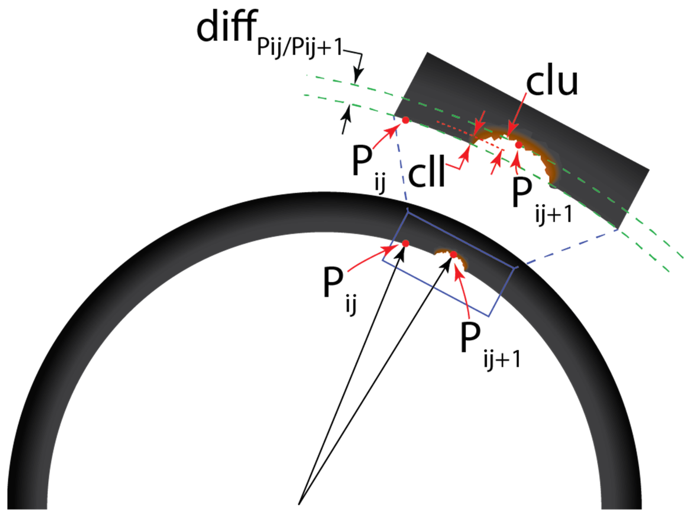
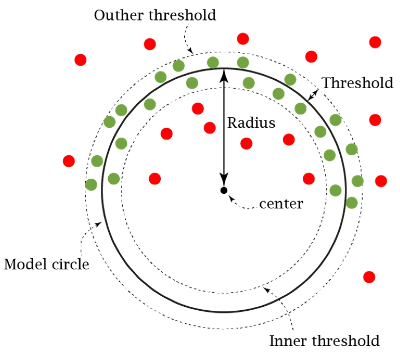
3.2. Segmentation Using the RANSAC-Modified Algorithm

Segmentation of 3D point clouds often has to deal with the problem of defining the differences or edges between the foreground and background due to the entanglements that exist between these in a so-called “scene” [31]. In the case of a pipeline internal surface scan, this problem is reduced due to the known ideal cylindrical shape of the pipeline, which can be modeled and easily label as background, leaving all data that does not fulfill the background characteristics as a foreground, and therefore “defects” or “non-desired surfaces”. Random Sample Consensus (RANSAC) is a method utilized for the calculation of a model that fits a set of data, without outliers affecting the result. With this, we can identify the outliers in our data (the pipes’ point cloud). The algorithm has been utilized for point cloud analysis in research like [32,33,34], since presented in [35].

In our case, the model to be fit is a circle in (19), in order to find the diameter and center of the inspected pipeline. In addition, the objective of using the algorithm is the augmentation of the useful data in the point cloud to present the final result [11].

$$\begin{array}{c}{x}^2+y^2+2gx+2fy+c=0\\ r^2=g^2+f^2-c\end{array}$$

(19)

Equation (19) is the mathematical model for the circle profile there, $x,y$ are the spatial coordinates of the evaluated point, $r$ is the radius of the circle model, and $c$, $f$, and $g$ are the circle’s center constants.

The algorithm iterates by randomly selecting a subset from the point cloud to be analyzed, fitting the model (19) to the selected subset with a determined threshold distance, determining the number of outliers (data outside the threshold), and repeating steps for k iterations.

Figure 9 is the representation of the RANSAC algorithm. In the Figure, outliers are represented in red, inliers in blue, and the circle to be fit in black.

With the application of RANSAC, the conditions of the pipe can be determined in a logical, natural way. The Experimental Evaluation Section of the paper presents the results after modification to the algorithm for defect identification. If the identification is not possible, the algorithm in Figure 8 determines if a higher density of data (more 3D points measured in a minor area) scan should be taken in the highlighted zone to accurately identify the defect and decide if future maintenance is needed.

Inliers, used for a pipe’s parameter determination, and the identification of outliers, result from point cloud evaluation using RANSAC. The outliers are evaluated for condition in (20).

$$\begin{array}{l}outlier>radius=outlier\\ outlier<radius=possibledefect\end{array}$$

(20)

After the condition evaluation, outliers are eliminated from the final point cloud, and possible defects are evaluated with the nearest neighborhood, such as that presented in [10]. If the data points are far apart from each other, they remain as outliers, and are eliminated from the point cloud. If enough points are gathered in a zone, they are classified as defects according to the Table below.

Table 2. Failure/defect classification.

Failure	Defect Location	Probability
Corrosion	Internal	High
Weld Failure	Internal	Small
Perforation	Internal/External	Medium
Crack	Internal/External	Medium
Manufacturing Defects	Internal	Small
Fracture	Internal	Medium

is the characteristic probability of an event. This information becomes critical in the robot’s setup and initialization, depending on the type of maintenance.

These three processes for the pipe scanning are continuously repeated until the full pipeline segment scan is finished.

4. Experimental Evaluation

4.1. Considerations

An important point to consider about the prototype is the software and hardware architecture used to control all the elements. The software for the inspection system uses MATLAB R2023b for surface evaluation, 3D measurements, and signal processing, and Python for operation algorithm programing and RANSAC application. The acquisition and preprocess stages are performed with a microcontroller, and the acquired data are saved to an onboard memory to be accessible at any moment. For hardware, the used accelerometric platform is the MPU6050, the stop sensor on the SA is the BPW77NB, a Teensy 4.1 USB is used to acquire the signals, and an Arduino MEGA is used for MR movement. The selected MR movement is the skid steer movement, where the opposite rotation of robot wheels perform movement and can achieve rotation of the system. The Arduino sends movement signals to a h-bridge driver and enables wheel rotation. Depending on the situation, the rotation could be clockwise or counterclockwise. Wheel rotation velocity is controlled with a pulse-width modulation (PWM) sent to the driver, also forming the Arduino.

The system has been tested in different conditions and experimental setups. This was to validate the functionality and accuracy of the developed scan methods. In addition, measurements were compared to those treated as ground-truth data (blueprint) to validate the inspection method’s operation error. The most important factors obtained during the experiments are accuracy on said conditions, 3D map quality, defect identification, detection of spatial orientation, its performance in a real-time scale, and system robustness estimation.

4.1.1. Surface Sensor Suite Validation/Scanning Circular

One of the main problems to address in a scanning process inside a pipeline with the TVS is the processing part of the data received using the TVS. Due to the pipeline’s circular surface and material, the expected reflection of the emitting laser will be different from the ideal. This means that a validation of the data reflection received needs to be conducted.

To validate the use of the SA for inspection of the inner circular surface of the pipeline, a pipeline model was used. The TVS was first introduced alone in the pipeline model, and several experiments were carried out. Artificial defects and contaminants were added to the pipeline model to analyze the TVS performance under such circumstances. Different TVS positions inside the pipeline were tested for their benefit from the FOV accuracy zones. The received signals from the SA and the light-detector photometer were tested to determine their optimal interaction quality.

4.1.2. Measurements Validation

The measurements taken using the TVS were compared to the ones performed with the distance meter from Leica DISTO D810 and a Vernier (for smaller distances). Here are presented the differences between measures taken in experimental conditions from real ones. All the measurements acquired in experimental conditions (with different scanning speeds) are analyzed, and statistical data of them can provide valuable information in regard to the TVS performance under different conditions. Accuracy comparison between both TVS positions, at the time when the measurements were taken, concludes with the TVS ideal configuration to realize the surface scanning of the pipeline.

Defects such as pipeline deformities, perforations, and obstacles are successfully detected and identified. These are one of the most critical defects to be found and repaired in a pipeline that transports high-value resources.

4.1.3. Performance Evaluation with Existing Technologies

The performance of the whole system as a unit is evaluated and compared against the proposals from the literature. In [17], a corroded metal pipe of diameter 600 mm was used to test their method with an accuracy of 1 mm. Other literature, such as [17,18,19], present an accuracy of around 7 mm.

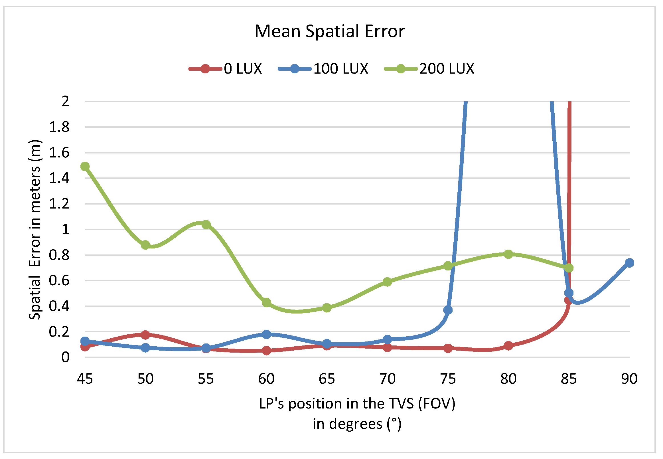
4.2. Measurements under Different Light Conditions

For the generality of the obtained results, the multiparametric optical TVS functioning was tested measuring the same during the different illumination conditions in the inspection zone. It was provided for three different levels of external light: 0 lux (with a turned-off light in the laboratory, and totally covered by dark curtains on the pipeline’s prototype), 100 lux (with a turned-off light in the laboratory, and partially covered by dark curtains on the pipeline’s prototype measuring the light condition using a photometer), and 200 lux (with a turned-on light in the laboratory, and partially covered by dark curtains on the pipeline’s prototype). The illuminance measurement was acquired with the 407,026 Heavy Duty Light Meter from EXTECH. The results of this experiment are shown in Figure 10. According to [3,5,8,9], the TVS has a performance improvement under no-light environments. Experiments to demonstrate this were carried out. Figure 10 presents the mean angular error of the TVS in different zones of the FOV. This error on the detection angle of the TVS can produce spatial errors in the measured coordinates of up to 10 cm (for example, at 1 m distance between surface and TVS) for the 45° LP’s position on the FOV at 1 m from the scanned surface.

In Figure 10, it is possible to observe that there are angles in which the measurement error is smaller in the presence of an external light source (100 LUX). Nevertheless, the overall performance of the TVS in the entire FOV has a smaller angular error in most of zones in the absence of light sources (0 LUX). It confirms, in a practical experimental way, our previous hypothesis that a laser scanning multi-parametric robotic platform is a good solution for inspection in darkness.

Furthermore, the presence of external light sources affects the acquired signal, directly resulting in the necessity of filters or some other kinds of elements to reduce error or increase the capability of the TVS to reach longer distances.

In Figure 11, the influence of external light sources (blue) on the detection signal can be seen. The laser-reflected energy (signal represented in red) is surpassed by the light source, providing errors in the TVS measurements. The external light source influence on the signal produces a different error depending on the LP’s position in the FOV.

Figure 12 is the mean spatial error of the TVS in different light conditions. In Figure 12, it can be identified that the spatial error of the measurements taken with the TVS behave similar to the errors in Figure 10. In addition, due to the spatial error being the summarization of the coordinate measurement error in the three different axes, these errors could mean that the resulting point cloud will be less reliable.

Analyzing Figure 10 and Figure 12, and especially Figure 11, we can state a very important and novel contribution of the present work: in contrast to [1,15], we can simplify, without efficiency losses, the search of the most significant and dangerous damage of the pipeline, such as a complete perforation. We can conduct this with the artificial isolation of two complementary information flows; meanwhile, as the x, y, z coordinates of the scanned surface point come from the 3D laser scanner, the information about perforation comes from photosensor channel. When the signal shape in this informational channel changes instantly, such as the drastic change presented in Figure 11, the system detects the fault type “perforation” based only on an analysis of the optical conditions of lightening within in-pipeline darkness (this process is illustrated with operator “$l{l}_A$” in the flow chart of Figure 8). Meanwhile, the coordinates x, y, z of this fault location come traditionally from the first informational channel. This is the first novel finding of our proposed method. It permits us to simplify and accelerate the detection of this dangerous defect, in comparison to [1,15]. It is important to note that this is obtained thanks to the use of other physical principles, albeit, however, from the same optical sensory part. This permits us to classify our TVS as multiparametric inspection system. From these experiments, in conclusion, it is important to note that the environment conditions inside the pipeline are suitable for the natural performance improvement of the scanning system, since, the majority of the time, the inspection environment will be in complete darkness (close to 0 LUX) due to the absence of light sources (other than the laser).

4.3. Workspace

With the intent to replicate the application conditions of a pipeline inspection, a wooden semi-cylinder surface was made to simulate the pipeline, providing both a surface sample and darkness conditions (the simulated environments also reproduced the internal color condition and texture in controlled laboratory conditions). Therefore, practically, our device represents an optical laser scanner multi-parametric system mounted on an autonomous robotic platform, which uses a variable combination of various physical phenomenon to achieve a practical task, namely, to automatically detect defects occurring in large-scale pipelines.

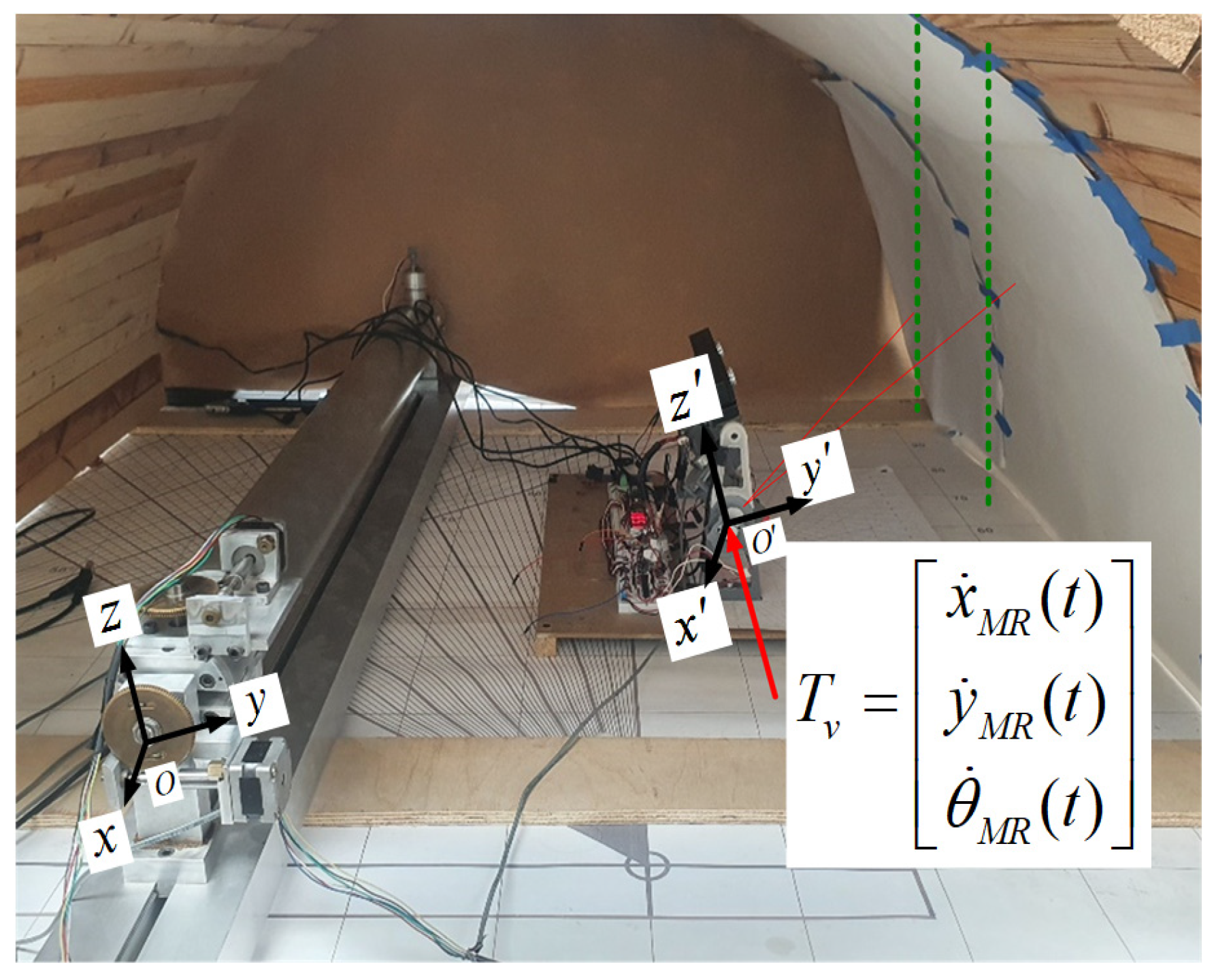
4.4. Acquisition Algorithm Validation-Data Acquisition in Motion

The scanning system was provided with measurement units, such as encoders (for the MR wheels), and the inertial platform (for the robot position changes), which were capable of displacement measurements and provided useful information about the MR surroundings, and which are utilized in the experimental stage of this paper.

In the following section, we describe an experimental setup made to perform an evaluation of precision and accuracy for the presented inspection method. Figure 5 shows the experimental setup used to validate the performance of the scanning method in dynamic conditions (using the mentioned approach of the displacement measurements, utilized as translation and rotation parameters for the individual scans taken with the TVS), as well as to demonstrate and quantify the advantage of the system working on different light conditions. In Figure 13, the MR moves inside the pipeline section (simulated with a wooden semi-cylinder surface, used to provide both surface sample and darkness chamber), and the TVS scans the inner surface of the pipeline. As mentioned before, the robot’s program is set to move at a quasi-static velocity (but still variable), giving the TVS enough time to perform scans. The TVS scans the internal pipeline section surface, and the robot’s odometer and the displacement measurement units store the motion data to apply the new position to the 3D data clouds measured using the TVS. The experiment consisted of different individual scans of the TVS. While the MR moves along the pipeline section length, it covers the entire surface of one lateral side of the pipeline. Figure 13 shows the generation of a pipeline’s section. With one third of battery power, the MR will travel along the pipeline. With the remaining power, it will return to its starting point, during its movement back to the starting point it will scan the other half of the pipe. The individual scans or side of the pipe are identified as iterations $S{S}_s$, where $s$ is the iteration number of the ongoing pipeline inspection or the inspected side.

At any scan iteration, the displacement measurement units store the actual position of the MR, and thus the TVS’s position (origin of coordinate system ${O^{\prime }}_{x^{\prime }{y}^{\prime }{z}^{\prime }}$) and every single point taken by the TVS is translated and rotated with Equation (16) to generate a full surface scan, combining both halves of these mentioned lateral side scans. The results of its junction in a complete point-cloud of the scanned pipeline is presented below in this text.

The inspection system acquires one side of the pipeline ($S{S}_s$) until the battery decreases to a set power level, $B_{l1}$. At that moment, the MR turns in its own vertical axis with a skid-steer-type movement. The orientation and position change of the MR is captured with the accelerometric platform and stored in $T_v$, and ${\dot{\theta }}_{MR}(t)$ matrixes with proper correspondence of $ij$. The opposite side of the pipe is acquired on the MR’s return to the beginning position of the inspection. With this functioning, the MR completely performs the pipe’s section inspection, and is capable of identifying defects in its profile.

Bearing in mind that the experiments to compare the TVS functioning in different operation modes were performed using the experimental setup in Figure 14, the static performance of the TVS prototype 2 (left on picture) was compare against the dynamic functioning of the TVS prototype 4 (right side, which is used for the inspection system of Figure 4).

In the experimental setup of Figure 14, the TVS prototype 2 is taken as the original coordinate system of reference $O$, and the prototype 4 is the $O^{\prime }$ moving coordinate system (moved in this experiment using a precise watch mechanism, joined with prototype 4 using a constantan wire), which is translated by  $T_v$. In comparison, the entire point cloud acquired with the prototype 2 can be evaluated using the RANSAC without point cloud adjustments, whereas the point cloud acquired with prototype 4 should be aligned after translations with $T_v$. This, due to deviation of the measured points in the FOVs, lowers the precision zones. Nonetheless, the resulting point cloud’s deviations do not affect the final result of the RANSAC evaluation. These experiments demonstrate that taking several individual point clouds and combining them with a reference position stored at any time in $T_v$ creates results that are useful for analysis of large scale pipes. The addition of the displacement measurement units of the MR to store the position changes in $T_v$ enables the inspection system to conform the internal pipeline surface due to the generation of the translation and rotation vectors that are used to shape the entire 3D point cloud.

According to previous experiments, the used accelerometric platform/gyroscope has a displacement error of 0.04 ± 0.01 mm to every single axis.

Figure 15 shows the point cloud acquired from the inspection made using the TVS in the experimental set up. As can be observed, the measured point cloud presents the inner surface curvature of the pipeline. Figure 16 shows the final point cloud acquired after the second side of the pipelines has been scanned and both have been adjusted using Equation (16). The TVS proves to be useful in the representation of the pipe’s cylindrical profile.

Due to setup constraints (we could only access to half of a pipe wooden model), the experimentation focused on real acquired data. Therefore, the point clouds and graphics presented are just the upper half of a pipe. However, for the lower part of the internal surface of the pipe, this algorithm will not differ significantly. It will just suppose some smaller mathematical changes in the assignment of the Cartesian coordinates. It is expedient to note that, for scanning efficiency to increase, the whole scanning can be divided and then composed by performing scanning during both travel parts, being the straight and the return pass.

After the first experiments, it is necessary to test the use of the RANSAC algorithm to identify outliers in the point clouds acquired using the inspection system and verify their efficiency in the identification of the pipeline condition. As explained in the methodology Section 3, the algorithm of Figure 8 will intend to verify the circular profile of the pipe in its operator “RANSAC”, verifying the condition (20). Then, adding to this process axis of time, we will verify the cylindrical profile of the whole pipe.

By profiling point-clouds into circles, it was possible to obtain the following results.

The left graphic in Figure 17 shows the first profile fitting with the algorithm unaltered and with a threshold of 0.01 mm. As can be observed, most of the points were tagged or identified as outliers; this is due to the TVS intrinsic error in measurements. In the middle graph of Figure 17, the profiling result after adjusting the threshold to the measurement spatial error of the TVS is shown, which is 0.5 mm. In this case, 87% of the original point cloud is used to evaluate the pipe’s conditions. With the adjustment of the threshold, the RANSAC successfully identifies outliers that are far from the point cloud that defines the pipe. In this case, the algorithm identifies the circle parameters correctly: diameter and center. Is important to notice that, to identify the dimensions of the pipeline with the point cloud, most of the points in the cloud would not be useful, since the intrinsic error deviations of the TVS measurements will produce a distorted cloud. Therefore, a post-process of the point cloud to acquire the pipe dimensions and characteristics would be needed. Therefore, this experiment demonstrated the utility of the RANSAC algorithm to the specific application. The algorithm gets modified to classify outliers in different ways depending on certain conditions. Figure 17, right graph, shows the point cloud taken with the presence of a foam obstacle in the interior of the pipeline surface; after profiling the pipe dimensions, it is also noticed that a group of outliers in the interior of the circle represents an obstacle.

The second novel finding of our proposed method can be stated, also based on the analysis of Figure 17 and Figure 18. It is also mostly focused on the system robustness increase by means of a simplified and de-synthesized analysis algorithm. Really, as we can see in Figure 17, we can see several interesting aspects. The detected internal profile deformation (simulated in the experiment as a piece of foam mounted on the pipeline wall) can be recognized using the optical system as outliers of defect location. If the external outliers of Figure 17 are robustly deleted using RANSAC, by comparison, under the simple condition “point outside the detected profile or not”, the internal points of Figure 17 can be classified under a still simpler condition: the system is verifying (in the inspection-control algorithm of Figure 8) the density of points in this cloud of “internal outliers”. If the distance between such two adjacent outliers is more than the experimentally detected value Z = 3 cm, such points are really outliers, and its coordinates can be deleted from a memory of the inspection multisystem. But, if the distance between points is lower than Z, such a point cloud is the detected internal pipeline defect, and its 3D coordinates are immediately the ones of the localized deformation. The practical efficiency of such an original approach is confirmed and illustrated in Figure 18, where such a defect during the experiment was simulated using two separated pieces of foam mounted on the same inconvenient-for-scanning upper horizontal point of pipeline.

Finally, the third novel finding is the possibility that the independent wheeled mobile robotic platform system decouples the size of our MR from the own pipeline’s size, which permits us to practically explore the pipelines of different diameters or even with variable diameters, which is completely impossible, for example in method [13]. The cheap technology of 3D printing used for most parts of our mobile robotic platform multisystem, including parts of the optical 3D laser scanning TVS, in practice permits us to vary, almost without constrains, the size of our MR, adjusting it to any diameter of pipe.

5. Conclusions

This research presents an inspection methodology for the structural integrity estimation of pipelines using the TVS Laser Scanner. The main challenge of this work was to present a reduced mathematical formalism, which at the same time can help to reach two mutually exclusive objectives: permit the computational system to use less time and resources for computation, and attribute the robustness/insensitivity directly to the calculation stage, avoiding, in this way, the processing of redundant information for defect detection. Robust mathematics, in our case, is a synthetized term, aiming to highlight its relation to the term of robustness in control, where the lower sensitivity to different kinds of physical perturbances is achieved thanks to the consecutive application of two independent proposed mathematical tools: dynamic triangulation formalism for obtaining 3D point clouds of the scanned surface, and RANSAC algorithm formalism in order to simplify cut-off criterion for classified outliers. It has been determined that the measuring system (TVS) can meet the application requirements for the selected task. In addition, the collaborative work between the TVS and the MR is suitable for the in-site inspection of a pipeline.

According to the previous results presented in [11], the RANSAC algorithm helps in identifying a pipe’s profile using accelerated outlier recognition. Furthermore, as new experiments show, outlier identification becomes a logical preliminary stage for defect detection and classification according to the algorithm presented in Section 3. In addition, the point-cloud’s efficiency improves due to the natural properties of our original optical laser scanning system involved in the mobile robotic platform, which uses an estimation of cross-correlated physical parameters to detect a versality of defects in a pipeline.

Thanks to the simplified and robust algorithm of the outliers’ detection, our optical system obtained the ability to detect the profile changes with appropriate uncertainty. Due to its robustness, the MR can perform the inspection and 3D surface measurements in a movement without losses of confidence, which enhances the inspection’s practical efficiency.

RANSAC’s application has two advantages: that already mentioned in [11] of a higher measured point’s utilization (point cloud’s efficiency), and the possibility of defect classification by analyzing the outliers’ relative position concerning the circle profile’s center. Experimental results in [11] demonstrate that using a threshold level of 0.5 mm increases the useful point quantity to 80.87% from a point cloud sample of 800 measurements. Nevertheless, in the same previous research, the percentage of potential defects in the total point cloud was 17.82%; by applying the detection algorithm developed in Section 3, the outlier percentage of potential defects results in 16.79%. This is due to the outliers’ evaluation with the neighborhood algorithm and radial distance from the circle profile’s center.

System efficiency is considered to be enhanced by giving utility to most measurements, and by the avoidance of extra scanning and processing stages for a pipes’ feature analysis.

Prototype and Further Applications

The following observations are research areas where the system could improve in future work. They are as follows: Firstly, modification to the RANSAC algorithm to cylinder fitting (instead of circle profiles) for defect classification; this would be to compare both fitting performances and find the optimized operation. Secondly, the $k$ variable (sample number) average; it is significant in the precision improvement of the TVS measurements to be able to improve this, and the SA, PL, and the Teensy-sampling rate of the TVS should improve or be optimized.

References

1. Shukla, A.; Karki, H. Application of Robotics in Onshore Oil and Gas Industry-A Review Part I. Rob. Auton. Syst. 2016, 75, 490–507. [Google Scholar] [CrossRef]
2. Abubakar, S.A.; Mori, S.; Sumner, J. A Review of Factors Affecting SCC Initiation and Propagation in Pipeline Carbon Steels. Metals 2022, 12, 1397. [Google Scholar] [CrossRef]
3. Sergiyenko, O.; Hernandez, W.; Tyrsa, V.; Cruz, L.F.D.; Starostenko, O.; Peña-Cabrera, M. Remote Sensor for Spatial Measurements by Using Optical Scanning. Sensors 2009, 9, 5477–5492. [Google Scholar] [CrossRef] [PubMed]
4. Sergiyenko, O.Y.; Tyrsa, V.V. 3D Optical Machine Vision Sensors with Intelligent Data Management for Robotic Swarm Navigation Improvement. IEEE Sens. J. 2021, 21, 11262–11274. [Google Scholar] [CrossRef]
5. Básaca-Preciado, L.C.; Sergiyenko, O.Y.; Rodríguez-Quinonez, J.C.; García, X.; Tyrsa, V.V.; Rivas-Lopez, M.; Hernandez-Balbuena, D.; Mercorelli, P.; Podrygalo, M.; Gurko, A.; et al. Optical 3D Laser Measurement System for Navigation of Autonomous Mobile Robot. Opt. Lasers Eng. 2014, 54, 159–169. [Google Scholar] [CrossRef]
6. Santos-Sanchez, J.O.; Rojas-Casas, M.A.; Sergiyenko, O.; Rodriguez-Quinonez, J.C.; Flores-Fuentes, W.; Sepulveda-Valdez, C.; Alaniz-Plata, R.; Tyrsa, V.; Mercorelli, P. Analysis of the Construction of an Autonomous Robot to Improve Its Energy Efficiency When Traveling through Irregular Terrain. In Proceedings of the IECON 2022—48th Annual Conference of the IEEE Industrial Electronics Society, Brussels, Belgium, 17–20 October 2022. [Google Scholar] [CrossRef]
7. Alaniz-Plata, R.; Sergiyenko, O.; Flores-Fuentes, W.; Tyrsa, V.V.; Rodríguez-Quiñonez, J.C.; Sepúlveda-Valdez, C.A.; Andrade-Collazo, H.; Mercorelli, P.; Lindner, L. ROS and Stereovision Collaborative System. In Optoelectronic Devices in Robotic Systems; Springer: Cham, Switzerland, 2022; pp. 71–113. [Google Scholar] [CrossRef]
8. Sergiyenko, O. Optoelectronic Devices in Robotic Systems; Springer: Cham, Switzerland, 2022; ISBN 9783031097911. [Google Scholar]
9. Sepulveda-Valdez, C.; Sergiyenko, O.; Tyrsa, V.; Flores-Fuentes, W.; Rodriguez-Quinonez, J.C.; Murrienta-Rico, F.N.; Miranda-Vega, J.E.; Mercorelli, P.; Kolendovska, M. Geometric Analysis of a Laser Scanner Functioning Based on Dynamic Triangulation. In Proceedings of the 2020 IEEE 29th International Symposium on Industrial Electronics (ISIE), Delft, The Netherlands, 17–19 June 2020; pp. 1398–1403. [Google Scholar] [CrossRef]
10. Real-Moreno, O.; Castro-Toscano, M.J.; Rodríguez-Quiñonez, J.C.; Hernández-Balbuena, D.; Flores-Fuentes, W.; Rivas-Lopez, M. Implementing K-Nearest Neighbor Algorithm on Scanning Aperture for Accuracy Improvement. In Proceedings of the IECON 2018—44th Annual Conference of the IEEE Industrial Electronics Society, Washington, DC, USA, 21–23 October 2018; pp. 3182–3186. [Google Scholar] [CrossRef]
11. Sepulveda-Valdez, C.; Sergiyenko, O.; Alaniz-Plata, R.; Núñez-López, J.A.; Tyrsa, V.; Flores-Fuentes, W.; Rodriguez-Quiñonez, J.C.; Mercorelli, P.; Kolendovska, M.; Kartashov, V.; et al. Laser Scanning Point Cloud Improvement by Implementation of RANSAC for Pipeline Inspection Application. In Proceedings of the IECON 2023—49th Annual Conference of the IEEE Industrial Electronics Society, Singapore, 16–19 October 2023; pp. 1–6. [Google Scholar]
12. PEMEX Base de Datos Institucional|Estadísticas Operativas Seleccionadas. Available online: https://ebdi.pemex.com/bdi/bdiController.do?action=cuadro&cvecua=MESTADOP (accessed on 16 November 2022).
13. Mathieson, W.L.; Croft, P.; Wuttig, F.J. Infrastructure Adaptions to Changing Permafrost Conditions—Three Case Studies along the Trans Alaska Pipeline System. In Proceedings of the Geo-Congress 2020: Geotechnical Earthquake Engineering and Special Topics, Minneapolis, MN, USA, 25–28 February 2020; pp. 913–925. [Google Scholar]
14. Shukla, A.; Xiaoqian, H.; Karki, H. Autonomous Tracking of Oil and Gas Pipelines by an Unmanned Aerial Vehicle. In Proceedings of the 2016 IEEE 59th International Midwest Symposium on Circuits and Systems (MWSCAS), Abu Dhabi, United Arab Emirates, 16–19 October 2016. [Google Scholar]
15. Kim, J.H.; Sharma, G.; Iyengar, S.S. FAMPER: A Fully Autonomous Mobile Robot for Pipeline Exploration. In Proceedings of the 2010 IEEE International Conference on Industrial Technology, Via del Mar, Chile, 14–17 March 2010; pp. 517–523. [Google Scholar] [CrossRef]
16. Roslin, N.S.; Anuar, A.; Jalal, M.F.A.; Sahari, K.S.M. A Review: Hybrid Locomotion of in-Pipe Inspection Robot. Procedia Eng. 2012, 41, 1456–1462. [Google Scholar] [CrossRef]
17. Gunatilake, A.; Piyathilaka, L.; Tran, A.; Vishwanathan, V.K.; Thiyagarajan, K.; Kodagoda, S. Stereo Vision Combined with Laser Profiling for Mapping of Pipeline Internal Defects. IEEE Sens. J. 2021, 21, 11926–11934. [Google Scholar] [CrossRef]
18. Latif, J.; Shakir, M.Z.; Edwards, N.; Jaszczykowski, M.; Ramzan, N.; Edwards, V. Review on Condition Monitoring Techniques for Water Pipelines. Measurement 2022, 193, 110895. [Google Scholar] [CrossRef]
19. Tan, K.; Cheng, X. Correction of Incidence Angle and Distance Effects on TLS Intensity Data Based on Reference Targets. Remote Sens. 2016, 8, 251. [Google Scholar] [CrossRef]
20. Lopez, M.R.; Sergiyenko, O.Y.; Tyrsa, V.V.; Perdomo, W.H.; Cruz, L.F.D.; Balbuena, D.H.; Burtseva, L.P.; Hipolito, J.I.N. Optoelectronic Method for Structural Health Monitoring. Struct. Health Monit. 2009, 9, 105–120. [Google Scholar] [CrossRef]
21. MX344504 Sistema Optico de Triangulacion Dinamica Para la Medicion de Angulos y Coordenadas en un Espacio Tridimensional. Available online: https://patentscope.wipo.int/search/en/detail.jsf?docId=MX152798571&recNum=1&maxRec=2&office=&prevFilter=&sortOption=Pub+Date+Desc&queryString=FP%3A%28Sistema+AND+Triangulacion+AND+Dinamica%29&tab=NationalBiblio (accessed on 5 June 2024).
22. Núñez-Lónez, J.A.; Sergiyenko, O.; Alaniz-Plata, R.; Sepulveda-Valdez, C.; Peréz-Landeros, O.M.; Tyrsa, V.; Flores-Fuentes, W.; Rodriguez-Quiñonez, J.C.; Murrieta-Rico, F.N.; Mercorelli, P.; et al. Advances in Laser Positioning of Machine Vision System and Their Impact on 3D Coordinates Measurement. In Proceedings of the IECON 2023—49th Annual Conference of the IEEE Industrial Electronics Society, Singapore, Singapore, 16–19 October 2023; pp. 1–6. [Google Scholar]
23. Latoui, A.; Hossine Daachi, M.E. Implementation of Q-Learning Algorithm on Arduino: Application to Autonomous Mobile Robot Navigation in COVID-19 Field Hospitals. In Proceedings of the International Conference on Electrical, Computer, and Energy Technologies, ICECET 2021, Cape Town, South Africa, 9–10 December 2021. [Google Scholar]
24. Febbo, R.; Flood, B.; Halloy, J.; Lau, P.; Wong, K.; Ayala, A. Autonomous Vehicle Control Using a Deep Neural Network and Jetson Nano. In Proceedings of the ACM International Conference Proceeding Series, Portland, OR, USA, 26 July 2020; Association for Computing Machinery: New York, NY, USA, 2020; pp. 333–338. [Google Scholar]
25. Vespoli, S.; Guizzi, G.; Converso, G.; Popolo, V.; Tedesco, A. An Electrical DC Motor Equivalent Circuit Testbed for the Battery Prognostic Health and Management. In Proceedings of the 2019 IEEE International Workshop on Metrology for Industry 4.0 and IoT, MetroInd 4.0 and IoT 2019—Proceedings, Naples, Italy, 4–6 June 2019; pp. 108–111. [Google Scholar]
26. Singh, S.; Weeber, M.; Birke, K.P. Advancing Digital Twin Implementation: A Toolbox for Modelling and Simulation. In Proceedings of the Procedia CIRP, Gulf of Naples, Italy, 1 January 2021; Elsevier: Amsterdam, The Netherlands, 2021; Volume 99, pp. 567–572. [Google Scholar]
27. Wang, Z.; Cao, Q.; Luan, N.; Zhan, L. Development of an Autonomous In-Pipe Robot for Offshore Pipeline Maintenance. Ind. Rob. 2010, 37, 177–184. [Google Scholar] [CrossRef]
28. Hernandez, W.; de Vicente, J.; Sergiyenko, O.Y.; Fernández, E. Improving the Response of Accelerometers for Automotive Applications by Using LMS Adaptive Filters: Part II. Sensors 2010, 10, 952–962. [Google Scholar] [CrossRef] [PubMed]
29. Nayak, A.; Pradhan, S.K. Design of a New In-Pipe Inspection Robot. Procedia Eng. 2014, 97, 2081–2091. [Google Scholar] [CrossRef]
30. Capula Colindres, S.; Méndez, G.T.; Velázquez, J.C.; Cabrera-Sierra, R.; Angeles-Herrera, D. Effects of Depth in External and Internal Corrosion Defects on Failure Pressure Predictions of Oil and Gas Pipelines Using Finite Element Models. Adv. Struct. Eng. 2020, 23, 3128–3139. [Google Scholar] [CrossRef]
31. Nguyen, A.; Le, B. 3D Point Cloud Segmentation: A Survey. In Proceedings of the 2013 6th IEEE Conference on Robotics, Automation and Mechatronics (RAM), Manila, Philippines, 12–15 November 2013; pp. 225–230. [Google Scholar] [CrossRef]
32. Schnabel, R.; Wahl, R.; Klein, R. Efficient RANSAC for Point-cloud Shape Detection. In Computer Graphics Forum; Blackwell Publishing Ltd.: Oxford, UK, 2007; Volume 26, pp. 214–226. [Google Scholar] [CrossRef]
33. Martínez-Otzeta, J.M.; Rodríguez-Moreno, I.; Mendialdua, I.; Sierra, B. RANSAC for Robotic Applications: A Survey. Sensors 2022, 23, 327. [Google Scholar] [CrossRef] [PubMed]
34. Li, J.; Hu, Q.; Ai, M. Point Cloud Registration Based on One-Point RANSAC and Scale-Annealing Biweight Estimation. IEEE Trans. Geosci. Remote Sens. 2021, 59, 9716–9729. [Google Scholar] [CrossRef]
35. Fischler, M.A.; Bolles, R.C. Random Sample Consensus: A Paradigm for Model Fitting with Applications to Image Analysis and Automated Cartography. Commun. ACM 1981, 24, 381–395. [Google Scholar] [CrossRef]
Figure 1. A 3D model of the Scanning System (TVS). (a) Active Node. (b) Sensing Node.
Mathematics 12 01940 g001
Figure 2. Scanning Aperture (SA) diagram.
Mathematics 12 01940 g002
Figure 3. Dynamic triangulation top view.
Mathematics 12 01940 g003
Figure 4. The Pipeline Inspection System’s Hardware—3D Model. (A) is the cross section of the Scanning Aperture (SA). (B) is the cross section of the Laser Positioner (LP).
Mathematics 12 01940 g004
Figure 5. Representation of the Pipeline Scanning System’s physical variables (in a wooden construction for modeling the pipeline segment).
Mathematics 12 01940 g005
Figure 6. dmin representation on dynamic triangulation.
Mathematics 12 01940 g006
Figure 7. Corrosion failure graphic representation.
Mathematics 12 01940 g007
Figure 8. General workflow of the Inspection System with the exploration path algorithm, the Surface Scan algorithm, and the Point Cloud Segmentation using RANSAC.
Mathematics 12 01940 g008
Figure 9. RANSAC algorithm representation.
Mathematics 12 01940 g009
Figure 10. Mean Angular Error for different light conditions. Illuminance of the Environment 0 LUX (red), 100 LUX (blue), 200 LUX (green). Sample of 3000 measurements.
Mathematics 12 01940 g010
Figure 11. Example of signal with the presence of the light source’s (in blue) visible light entire wavelength. Part of the signal of a 633 nm wavelength. Representation of the signal in total darkness (red).
Mathematics 12 01940 g011
Figure 12. Mean Spatial error.
Mathematics 12 01940 g012
Figure 13. Representation of Scanning Algorithm in the experimental setup. Point cloud generation with MR’s displacement.
Mathematics 12 01940 g013
Figure 14. Experimental setup. Evaluation of displacement measurement units.
Mathematics 12 01940 g014
Figure 15. Result of the scan for one side (half) of the pipeline. Point cloud: 1400 measurements.
Mathematics 12 01940 g015
Figure 16. Entire pipeline section after second scan. Point cloud: 2792 measurements.
Mathematics 12 01940 g016
Figure 17. First profile fitting with RANSAC, threshold (t = 0.01 mm). Ideal, red: Outliers (will be eliminated from the result), and blue (Inliers) will be kept for the result. Second profile fitting with RANSAC, threshold (t = 0.5 mm). TVS mean error, red: Outliers (will be eliminated from the result), and blue (Inliers) will be kept for the result. Third profile fitting with RANSAC, threshold (t = 0.5 mm). Red (Outliers), and blue (Inliers).
Mathematics 12 01940 g017
Figure 18. Fourth profile fitting with RANSAC, threshold (t = 0.5 mm). Green (Inliers); red + (Outliers) with Distance to Circle’s center method; red circle (Outliers) with k-nearest neighbor method; and blue (possible object). Point cloud junction at the top of the circle’s profile.
Mathematics 12 01940 g018