Article

Dynamical Behaviors and Abundant New Soliton Solutions of Two Nonlinear PDEs via an Efficient Expansion Method in Industrial Engineering

1
Department of Mathematics, Faculty of Science, Islamic University of Madinah, Madinah 42351, Saudi Arabia
2
Department of Mathematics, Bangladesh Army University of Engineering and Technology, Natore 6431, Bangladesh
3
Administrative and Financial Science Department, Ranyah University College, Taif University, P.O. Box 11099, Taif 21944, Saudi Arabia
4
Technology and Science Department, Ranyah University College, Taif University, P.O. Box 11099, Taif 21944, Saudi Arabia
5
Department of Mathematics, Jashore University of Science and Technology, Jashore 7408, Bangladesh
6
Division of Mathematical and Physical Sciences, Kanazawa University, Kanazawa 9201192, Japan
7
Department of Mathematics, Khulna University of Engineering & Technology, Khulna 9203, Bangladesh
8
Department of Industrial Engineering, College of Engineering, University of Business and Technology, Jeddah 21448, Saudi Arabia
9
Department of Mechanical Engineering, College of Engineering, Zarqa University, Zarqa 13110, Jordan
*
Authors to whom correspondence should be addressed.
Mathematics 2024, 12(13), 2053; https://doi.org/10.3390/math12132053
Submission received: 27 May 2024 / Revised: 26 June 2024 / Accepted: 27 June 2024 / Published: 30 June 2024
(This article belongs to the Special Issue Exact Solutions and Numerical Solutions of Differential Equations)

Abstract

:
In this study, we discuss the dynamical behaviors and extract new interesting wave soliton solutions of the two significant well-known nonlinear partial differential equations (NPDEs), namely, the Korteweg–de Vries equation (KdVE) and the Jaulent–Miodek hierarchy equation (JMHE). This investigation has applications in pattern recognition, fluid dynamics, neural networks, mechanical systems, ecological systems, control theory, economic systems, bifurcation analysis, and chaotic phenomena. In addition, bifurcation analysis and the chaotic behavior of the KdVE and JMHE are the main issues of the present research. As a result, in this study, we obtain very effective advanced exact traveling wave solutions with the aid of the proposed mathematical method, and the solutions involve rational functions, hyperbolic functions, and trigonometric functions that play a vital role in illustrating and developing the models involving the KdVE and the JMHE. These new exact wave solutions lead to utilizing real problems and give an advanced explanation of our mentioned mathematical models that we did not yet have. Some of the attained solutions of the two equations are graphically displayed with 3D, 2D, and contour panels of different shapes, like periodic, singular periodic, kink, anti-kink, bell, anti-bell, soliton, and singular soliton wave solutions. The solutions obtained in this study of our considered equations can lead to the acceptance of our proposed method, effectively utilized to investigate the solutions for the mathematical models of various important complex problems in natural science and engineering.

1. Introduction

In recent centuries, NPDEs have been significantly employed to illustrate nonlinear phenomena in many complex sectors of the natural sciences, particularly in all fields of engineering and mathematical physics. The NPDEs are represented as the mathematical models of various important natural problems in the distinct fields of science and engineering. In modern science and engineering, a special NPDE class that has time dependency is called the nonlinear evolution equations (NEEs), which are discussed and analyzed using soliton solutions in the present study. For the past few decades, NEEs have played a very significant role in understanding the behavior of nonlinear wave problems that appear in plasma physics, chemical physics, biology, optical fibers, geochemistry, and chemical kinematics. The exact wave solutions of NEEs are very important for developing, analyzing, and solving mathematical models. The researchers are fond of investigating the wave solutions for NEEs which lead a significant appearance in nonlinear mathematical physics. As a result, the wave solutions are able to clarify and develop the many problems in natural phenomena, for instance, solitary waves, vibration systems, thermal systems, and wave propagations. Over the last several years, various analytical methods came to be improved to estimate the wave solutions of NEEs. These analytical methods involve the exp-function method [1,2], the modified exponential function method [3], the modified extended tanh-function method [4,5], the improved modified extended tanh-function method [6], the Jacobi elliptic function expansion method [7], the extended Jacobi elliptic function expansion method [8,9], the first integral method [10,11,12], the extended homogeneous balance method [13], the homogeneous balance method [14,15], the inverse scattering method [16,17,18], the sub-ODE method [19,20], the generalized sub-ODE method [21], the Lie group analysis method [22,23,24], the Lie symmetry analysis [25,26,27] and so on. In this present study, we discuss and focus on the solutions of two very special nonlinear equations, namely, the KdVE and the JMHE. An intriguing nonlinear phenomenon that has implications in many areas, incorporating engineering, economics, telecommunication, ecology, and control theory, is the study of bifurcation and chaos behavior. In [28], the dynamical behavior of chaos as well as bifurcation analysis were observed for the Konno–Onno model. Tang [29] has studied the bifurcation studies with chaotic patterns for the (2+1)-dimensional stochastic coupled nonlinear Schrödinger system. In [30,31], chaotic nature and bifurcation phenomena were also analyzed for distinct models. As per our knowledge, one examined the chaotic character and the bifurcation facts for the KdVE and JMHE. On or after this interest, we would check out the chaotic nature and bifurcation phenomena of the proposed models. For the past few decades, KdVE has been considered a significant model of NPDE in the study of water waves like shallow water waves and ocean waves. The KdVE has several generalized novel perturbed space-time forms in ocean wave models. The KdVE serves as a versatile and powerful tool for modeling a wide range of wave phenomena in geophysical contexts. Its ability to describe nonlinear and dispersive effects makes it indispensable for understanding and predicting the behavior of various types of waves in the natural environment. The KdVE is extensively used to model shallow water waves, atmospheric and oceanic sciences, tsunami wave propagation in shallow waters, seismic waves, tidal bore analysis, wave dynamics in ice-covered waters, sea ice dynamics, climate change effects, and marine navigation. In [32], interaction solutions of a geophysical KdVE have already been identified. Some important, well-known geographical water wave models like KdVE are mentioned in the articles [33,34]. Very recently, Hou et al. [35] established the Rossby waves and their dynamics of the KdVE. The analytic solutions of the KdVE led a massive development as well as improvement of the mathematical models in the literature of water wave mechanics and continuum physics. The nonlinear (2+1)-dimensional JMHE finds applications in various fields of mathematical physics due to its ability to describe complex, multidimensional wave phenomena. Moreover, the JMHE is an NEE. Its necessity in fluid dynamics, nonlinear mathematical physics, plasma physics, nonlinear optics, Bose–Einstein condensates, solid-state physics, and geophysical fluid dynamics highlight its versatility and importance. The JMHE relates to energy-dependent potential like Schrodinger, and it is a significant model in nonlinear complex problems. Over the last few decades, many investigators have been trying to find exact solutions to the JMHE to develop a model associated with numerous problems in nonlinear physics and natural sciences. In [36], kink wave, anti-kink wave, and periodic wave solutions were examined of the JMHE. Furthermore, there are some effective nonlinear equations in the articles [37,38,39] that are generated by JMHE. Very recently, Akkilic et al. [40] magnificently detected the wave solutions with singular, non-topological, and singular periodic wave shapes of the JMHE. From the literature and to the best of our knowledge, no one has operated the mentioned expansion approach to discover the wave solutions of the KdVE and JMHE. Moreover, the examined outcomes from this present work have individual roles in the previously established solutions, and our outcomes have substantial use in numerous domains of nonlinear science. From this relevance, our main concentration is to estimate many new exact solutions of KdVE and JMHE by employing the proposed mathematical method [41,42,43,44]. Recently, M. Akher Chowdhury et al. [45] utilized the proposed mathematical method called the generalization of the method that is given in [46,47,48] to obtain the analytical solutions of two important NEEs.
The following sections in this study are arranged as follows: The proposed method is discussed in Section 2. Under Section 3, the proposed method is applied to construct the solutions of Equations (1) and (3). Bifurcation analysis is found in Section 4. Then, Section 5 describes chaotic nature. Graphical and physical interpretations of some obtained particular solutions of the two equations are prescribed in Section 6. Finally, the conclusion is given in Section 7.

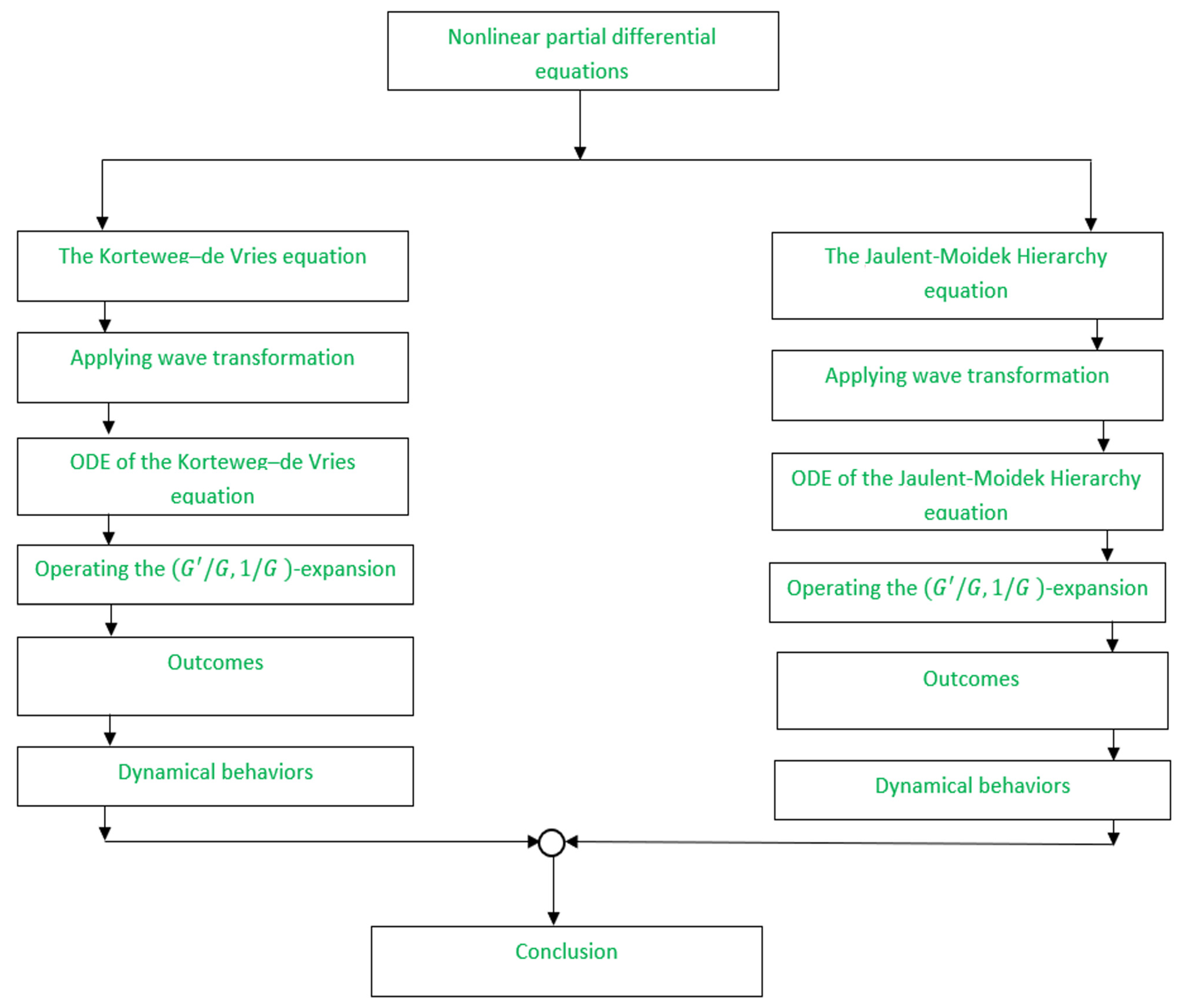
2. Basic Parts of the Proposed Method

We give a brief discussion of the proposed mathematical method [45,46,47,48]. To utilize the mentioned method, we first consider an equation, as follows:
G ζ + λ G ζ = q
In Equation (1), the prime notation leads to a second-order ordinary derivative of   G ζ , i.e., d 2 G d ζ 2 . Then for the substitutions   β = G / G , γ = 1 / G   into Equation (1), give the two relations as below:
β = β 2 + q γ λ ,   γ = β γ
Equation (1) leads to three exact solutions involving arbitrary constants   E 1 and E 2 . These exact solution functions are, respectively, performed for the negative, positive, and zero values of the parameter along with three respective important relations among   γ , λ , β , q , E 1 , and E 2 in Equations (3)–(5) along with Equations (6)–(8), respectively, as follows:
G ζ = E 1 s i n h λ ζ + E 2 c o s h λ ζ + q λ
G ζ = E 1 s i n λ ζ + E 2 c o s λ ζ + q λ
G ζ = q 2 ζ 2 + E 1 ζ + E 2
γ 2 = λ λ 2 σ 1 + q 2 ( β 2 2 q γ + λ )
γ 2 = λ λ 2 σ 2 q 2 ( β 2 2 q γ + λ )
γ 2 = 1 E 1 2 2 q E 2 ( β 2 2 q γ )
wherein σ 1 = E 1 2 E 2 2 as well as σ 2 = E 1 2 + E 2 2 .
Let us consider a polynomial equation of some higher-order partial derivatives, namely,
M h , h t , h x , h y , h t t , h y y , h x x , h y x , h t x , h t y , = 0
where h = h ( t , x ,   y ) . We convert the nonlinear polynomial Equation (9) into an ordinary differential equation (ODE), applying the following five axioms:
I. If we apply
h t , x , y = h ( ζ ) , ζ = c t + ε x + ϕ y
then the polynomial Equation (9) converts to ODE involving the constant coefficients   ε , ϕ , and c as below:
Z h , c h , ϕ h , ε h , ε 2 h , ε ϕ h , c ε h , ϕ 2 h , c 2 h , = 0
II. The assumed general solution involving the constant coefficients   a q ’s and   b q ’s of Equation (11) is as follows:
h ζ = a 0 + j = 1 K a j β j ζ + b j β j 1 ( ζ ) γ ( ζ )
where a K 2 + b K 2 0 .
III. The unknown integer number   K in Equation (12) is to be estimated by the rule of homogeneity.
IV. Obtaining the system of algebraic equations with unknowns   E 1 ,   E 2 ,   c ,   ϕ ,   ε ,   q ,   a 0 ,   a j ,   b j   ( j = 1 ,   2 ,   , K ) , and the negative value of λ generated by Mathematica, we use Equation (12) into Equation (11) along with the particular relations in Equations (2) and (6).
V. In a similar process described in axiom IV, the rest of the two general solutions of Equation (1) can be easily obtained. Following figure (Figure 1) is the flowchart.

3. Applications

In this section, we apply the mathematical method for constructing many new exact traveling wave solutions, which will be discussed throughout the following sections and subsections, of the two nonlinear wave equations that are mentioned in the former section.

3.1. The Nonlinear (1+1)-Dimensional Geophysical Korteweg–de Vries Equation

In this subsection, we explore the solutions of the nonlinear (1+1)-dimensional geophysical KdVE, which has several applications in shallow water waves, atmospheric and oceanic sciences, tidal bore analysis, wave dynamics in ice-covered waters, climate change effects, and marine navigation. Now let us consider the stated equation [36,37,38], as follows:
H t + ρ H x + α H H x + δ H x x x = 0 ,
where H = H x , t represents a particular free surface progress, ρ is a perturbation parameter applied for the Coriolis effect, α denotes the coefficient of nonlinearity, and   δ   indicates the dispersion factor involving complex wave phenomena.
We assume the transformation variable as
H x , t = H ζ , ζ = x c t ,
where   c   is the wave velocity of the solution. We therefore obtain the following ODE of Equation (13) with aid of the relations in Equation (14) as
c H ζ + δ H ζ α H ζ H ζ + ρ H ζ = 0 ,
where c   is the wave velocity of the solution. Integrating in Equation (15) in which the constant of integration is omitted, it can be converted into the following form as
c H ζ + δ H ζ 1 2 α H 2 ζ + ρ H ζ = 0 .
Applying axiom III, the general solution of Equation (16) for K = 2 is as follows:
H ζ = a 0 + a 1 β ζ + a 2 β 2 ζ + b 1 γ ζ + b 2 β ( ζ ) γ ( ζ ) ,
where   a 0 , a n , and b n   ( = 1 ,   2 ) are said to be the constant coefficients estimated later in such a way that   a K 2 + b K 2 0   ( K = 1 ,   2 ) . We justify the relations given in Equation (2) and obtain the three types of exact wave solutions computed in three different cases of Equation (16) as follows:
Case 1:
Performing axiom IV by Mathematica, it yields the following results for   λ < 0 along with   a 0 , a 1 ,   a 2 ,   b 1 ,   b 2 ,   c , and σ 1   as below,
Result 1:
a 0 = 4 δ λ α , a 1 = 0 ,   a 2 = 6 δ α , b 1 = 6 δ q α , b 2 = ± 6 δ q 2 + λ 2 σ 1 α λ , c = ρ + δ λ .
Plugging result 1 containing Equations (3) and (6) into Equation (17) provides a general wave solution as
H ζ = 4 δ λ α 6 δ λ E 1 c o s h λ ζ + E 2 s i n h λ ζ 2 α E 1 s i n h λ ζ + E 2 c o s h λ ζ + q λ 2 6 δ q α E 1 s i n h λ ζ + E 2 c o s h λ ζ + q λ ± 6 δ q 2 + λ 2 σ 1 { E 1 c o s h λ ζ + E 2 s i n h λ ζ } α { E 1 s i n h λ ζ + E 2 c o s h λ ζ + q λ } 2 ,
wherein ζ = x ( ρ + δ λ ) t and σ 1 = E 1 2 E 2 2 .
Letting   E 1 0 , E 2 = 0 , and q = 0 , Equation (18) becomes
H x , t = 4 δ λ α 6 δ λ α c o t h 2 λ x ( ρ + δ λ ) t ± 6 δ λ α c o t h λ x ( ρ + δ λ ) t c o s e c h λ x ( ρ + δ λ ) t .
Result 2:
a 0 = 6 δ λ α , a 1 = 0 , a 2 = 6 δ α , b 1 = 6 δ q α , b 2 = ± 6 δ q 2 + λ 2 σ 1 α λ , c = ρ δ λ .
In a similar fashion as the previous result, result 2 leads a general wave solution of Equation (16) as
H ζ = 6 δ λ α 6 δ λ E 1 c o s h λ ζ + E 2 s i n h λ ζ 2 α E 1 s i n h λ ζ + E 2 c o s h λ ζ + q λ 2 6 δ q α E 1 s i n h λ ζ + E 2 c o s h λ ζ + q λ ± 6 δ q 2 + λ 2 σ 1 { E 1 c o s h λ ζ + E 2 s i n h λ ζ } α { E 1 s i n h λ ζ + E 2 c o s h λ ζ + q λ } 2 ,
wherein ζ = x ( ρ δ λ ) t and σ 1 = E 1 2 E 2 2 .
Letting E 1 0 , E 2 = 0 , and q = 0 , Equation (20) becomes
H x , t = 6 δ λ α 6 δ λ α c o t h 2 λ x ( ρ δ λ ) t ± 6 δ λ α c o t h λ x ( ρ δ λ ) t c o s e c h λ x ( ρ δ λ ) t .
Case 2:
Executing axiom V, it yields the unknown constants   a 0 , a 1 , a 2 , b 1 , b 2 , c , and σ 2   for the parameter   λ > 0 in the following results as
Result 1:
a 0 = 4 δ λ α , a 1 = 0 , a 2 = 6 δ α , b 1 = 6 δ q α , b 2 = ± 6 δ λ 2 σ 2 q 2 α λ , c = ρ + δ λ .
The general solution of Equation (16) for result 1 is represented as
H ζ = 4 δ λ α + 6 δ λ E 1 c o s ζ λ E 2 s i n ζ λ 2 α E 1 s i n ζ λ + E 2 c o s ζ λ + q λ 2 6 δ q α E 1 s i n ζ λ + E 2 c o s ζ λ + q λ ± 6 δ λ 2 σ 2 q 2 { E 1 c o s ζ λ E 2 s i n ζ λ } α { E 1 s i n ζ λ + E 2 c o s ζ λ + q λ } 2 ,
wherein ζ = x ρ + δ λ t and σ 2 = E 1 2 + E 2 2 .
Letting   E 1 0 , E 2 = 0 , and q = 0 , Equation (22) executes
H x , t = 4 δ λ α + 6 δ λ α c o t 2 x ρ + δ λ t λ ± 6 δ λ α c o t x ρ + δ λ t λ c o s e c x ρ + δ λ t λ
Furthermore, letting   E 2 0 , E 1 = 0 , and q = 0 , Equation (22) gives
H x , t = 4 δ λ α + 6 δ λ α t a n 2 x ρ + δ λ t λ ± 6 δ λ α t a n x ρ + δ λ t λ s e c x ρ + δ λ t λ
Result 2:
a 0 = 6 δ λ α ,   a 1 = 0 ,   a 2 = 6 δ α ,   b 1 = 6 δ q α ,   b 2 = ± 6 δ λ 2 σ 2 q 2 α λ ,   c = ρ δ λ .
Similarly for result 2, the general solution of Equation (16) presents as
H ζ = 6 δ λ α + 6 δ λ E 1 c o s λ ζ E 2 s i n λ ζ 2 α E 1 s i n λ ζ + E 2 c o s λ ζ + q λ 2 6 δ q α E 1 s i n λ ζ + E 2 c o s λ ζ + q λ ± 6 δ λ 2 σ 2 q 2 { E 1 c o s ζ λ E 2 s i n ζ λ } α { E 1 s i n ζ λ + E 2 c o s ζ λ + q λ } 2 ,
wherein ζ = x ( ρ δ λ ) t and σ 2 = E 1 2 + E 2 2 .
Letting E 1 0 , E 2 = 0 , and q = 0 , Equation (25) grants
H x , t = 6 δ λ α c o s e c 2 x ρ δ λ t λ ± 6 δ λ α c o t x ρ δ λ t λ c o s e c x ρ δ λ t λ
Similarly, letting   E 2 0 , E 1 = 0 , and q = 0 , Equation (25) forms
H x , t = 6 δ λ α s e c 2 x ρ δ λ t λ ± 6 δ λ α t a n x ρ δ λ t λ s e c x ρ δ λ t λ
Case 3:
Promoting axiom V, it yields the following result for λ = 0   with the unknown constants   a 0 , a 1 , a 2 , b 1 , b 2 , and c as
a 0 = 0 ,   a 1 = 0 ,   a 2 = 6 δ α ,   b 1 = 6 δ q α ,   b 2 = ± 6 δ E 1 2 2 q E 2 α ,   c = ρ .
The general solution for the above constants of Equation (16) presents as
H ζ = 6 δ q ζ + E 1 2 α q 2 ζ 2 + E 1 ζ + E 2 2 6 δ q α q 2 ζ 2 + E 1 ζ + E 2 ± 6 δ ( q ζ + E 1 ) E 1 2 2 q E 2 α q 2 ζ 2 + E 1 ζ + E 2 2 ,
wherein ζ = x ρ t .
Letting E 1 0 , E 2 = 0 , and q = 0 , Equation (28) forms
H x , t = 12 δ α x ρ t 2

3.2. The Nonlinear (2+1)-Dimensional Jaulent–Miodek Hierarchy Equation

In this subpart, we discover the solutions of the nonlinear (2+1)-dimensional JMHE, which has numerous uses in fluid dynamics, plasma physics, optics, Bose–Einstein condensates, and geophysical fluid dynamics. We pick this specified equation [42,44,49] as follows:
w t = 1 4 ( w x x 2 w 3 ) x 3 4 1 4 x 1 w y y + w x x 1 w y
where   w = w t ,   x ,   y   and   y   are an analytic function and the spatial variable, respectively, x 1 = d x is an inverse operator of x such that x 1 x = 1 = x x 1 , and x r t d t = x 1 x r ( x ) under the decaying condition at   . By omitting the integral term, we let   w = P x x ,   y ,   t into Equation (30), and then it becomes the following form:
P x t + 1 4 P x x x x 3 2 P x 2 P x x + 3 16 P y y + 3 4 P x x P y = 0 .
Let us assume that
P x , y , t = p ( ζ ) , ζ = c t + x + y
wherein c is the speed of wave. Substituting the transformation given in Equation (32) into Equation (31),
c d 2 p d ζ 2 + 1 4 d 4 p d ζ 4 3 2 d p d ζ 2 d 2 p d ζ 2 + 3 16 d 2 p d ζ 2 + 3 4 d 2 p d ζ 2 d p d ζ = 0
Integrating Equation (33) with the constant of integration taken zero yields,
16 c d p d ζ + 4 d 3 p d ζ 3 8 d p d ζ 3 + 3 d p d ζ + 6 d p d ζ 2 = 0
For the sake of simplicity, letting d p d ζ = u ζ into Equation (34), it provides
16 c u + 4 d 2 u d ζ 2 8 u 3 + 3 u + 6 u 2 = 0
Proceeding with axiom III, the general solution of Equation (35) for   K = 1 yields
u ζ = a 0 + a 1 β ζ + b 1 γ ζ
Utilizing Equation (1) in Equation (36), we attain three distinct categories of wave solutions of Equation (35) that are described below:
Case 1:
Performing IV by Mathematica, it yields the following results for λ < 0 along with the unknown constants a 0 , a 1 , b 1 , c , and σ 1 as:
Result 1:
a 0 = 1 4 , a 1 = ± 1 2 , b 1 = ± 16 q 2 + σ 1 4 , λ = 1 4 , c = 1 4 .
Plugging result 1 containing Equations (3) and (6) into Equation (36) provides the general wave solution as
u ζ = 1 4 ± λ E 1 c o s h ζ λ + E 2 s i n h ζ λ 2 E 1 s i n h ζ λ + E 2 c o s h ζ λ + q λ ± 16 q 2 + σ 1 4 E 1 s i n h ζ λ + E 2 c o s h ζ λ + q λ ,
wherein ζ = 1 4 t + x + y and σ 1 = E 1 2 E 2 2 .
Letting   E 1 0 , E 2 = 0 , and q = 0 , Equation (37) becomes
u ζ = 1 4 ± λ 2 c o t h λ ζ ± 1 4 c o s e c h λ ζ ,
wherein ζ = 1 4 t + x + y . After integrating Equation (38),
p ζ = ζ 4 ± 1 2 l n s i n h λ ζ ± 1 4 λ l n t a n h λ 2 ζ ,
wherein ζ = 1 4 t + x + y   and we assume the integrating constant is zero. In space form, Equation (39) becomes
P t , x , y = 1 4 ( 1 4 t + x + y ) ± 1 2 l n s i n h λ ( 1 4 t + x + y ) ± 1 4 λ l n t a n h λ 2 ( 1 4 t + x + y ) .
Furthermore, the exact traveling wave solution of Equation (30) is
w t , x , y = 1 4 ± 1 8 s e c h λ 2 1 4 t + x + y c o s e c h λ 2 1 4 t + x + y ± λ 2 coth λ 1 4 t + x + y
Result 2:
a 0 = 1 4 ,   a 1 = ± 1 ,   b 1 = 0 , q = 0 , λ = 1 16 ,   c = 1 4 .
In a similar fashion as the previous result, result 2 leads a general wave solution of Equation (35) as
u ζ = 1 4 ± λ E 1 c o s h λ ζ + E 2 s i n h λ ζ E 1 s i n h λ ζ + E 2 c o s h λ ζ
wherein ζ = 1 4 t + x + y and σ 1 = E 1 2 E 2 2 .
Letting E 1 0 , E 2 = 0 , and q = 0 , Equation (42) permits
u ζ = 1 4 ± λ c o t h λ ζ
wherein ζ = 1 4 t + x + y . After integrating Equation (43),
p ζ = ζ 4 ± l n s i n h λ ζ ,
wherein ζ = 1 4 t + x + y and we assume the integrating constant is zero. In space form, Equation (44) becomes
P t , x , y = 1 4 ( 1 4 t + x + y ) ± l n s i n h λ ( 1 4 t + x + y ) .
Furthermore, the exact traveling wave solution of Equation (30) is
w t , x , y = 1 4 ± λ c o t h λ ( 1 4 t + x + y )
Case 2:
Executing axiom V, it yields the unknown constants a 0 , a 1 , b 1 , c , and σ 2 for the parameter λ > 0 in the following results as:
Result 1:
a 0 = 0 ,   a 1 = 0 ,   b 1 = ± 2 λ σ 2 1 + 4 λ ,   q = ± λ σ 2 1 + 4 λ ,   c = 1 16 ( 4 λ 3 ) .
The general solution of Equation (35) is represented as
u ζ = 2 q E 1 s i n λ ζ + E 2 c o s λ ζ + q λ
After integrating Equation (47) and taking the constant of integration as zero,
ζ = 4 q λ q λ 2 E 1 2 E 2 2 t a n 1 q λ E 2 t a n ζ λ 2 q λ 2 E 1 2 E 2 2
wherein ζ = 1 16 ( 4 λ 3 ) t + x + y , q = ± λ σ 2 1 + 4 λ , σ 2 = E 1 2 + E 2 2 and we assume the integrating constant is zero.
Letting E 1 0 and E 2 = 0 , in space form, Equation (48) becomes
P t , x , y = 4 q λ q λ 2 E 1 2 t a n 1 q λ t a n λ 2 ( 1 16 ( 4 λ 3 ) t + x + y ) q λ 2 E 1 2 ,
wherein   q = ± λ E 1 1 + 4 λ . Furthermore, the exact traveling wave solution of Equation (30) is
w t , x , y = 2 q 2 s e c 2 λ 2 ( 1 16 ( 4 λ 3 ) t + x + y ) λ q λ 2 s e c 2 λ 2 ( 1 16 ( 4 λ 3 ) t + x + y ) E 1 2 ,
wherein q = ± λ E 1 1 + 4 λ .
Result 2:
a 0 = 1 4 , a 1 = 0 , b 1 = ± σ 2 2 2 ,   q = 0 , λ = 1 8 , c = 1 4 .
Similarly, for result 2, the general solution of Equation (35) presents as
u ζ = 1 4 ± σ 2 2 2 E 1 s i n λ ζ + E 2 c o s λ ζ ,
wherein ζ = 1 4 t + x + y , λ = 1 8 , and σ 2 = E 1 2 + E 2 2 .
Letting E 1 0 and E 2 = 0 , Equation (51) grants
u ζ = 1 4 ± 1 2 2 c o s e c λ ζ ,
wherein ζ = 1 4 t + x + y and λ = 1 8 . After integrating Equation (52),
p ζ = ζ 4 ± 1 2 2 λ l n t a n λ ζ 2 ,
wherein ζ = 1 4 t + x + y , λ = 1 8 and we assume the integrating constant is zero. In space form, Equation (53) becomes
P t , x , y = 1 4 ( 1 4 t + x + y ) ± l n t a n 1 4 2 ( 1 4 t + x + y ) .
Furthermore, the exact traveling wave solution of Equation (30) is
w t , x , y = 1 4 ± 1 4 2 c o s e c 1 4 2 ( 1 4 t + x + y ) s e c 1 4 2 ( 1 4 t + x + y ) .
Case 3:
Promoting axiom V, it yields the following result for λ = 0 , exacting the constants   a 0 , a 1 , b 1 , c , and q as
a 0 = 0 ,   a 1 = 0 ,   b 1 = 1 2 E 2 ± 4 E 1 2 + E 2 2 ,   c = 3 16 ,   q = 1 4 E 2 ± 4 E 1 2 + E 2 2 .
The general solution for the above constants of Equation (35) presents as
u ζ = E 2 ± 4 E 1 2 + E 2 2 2 q 2 ζ 2 + E 1 ζ + E 2 ,
wherein ζ = 3 16 t + x + y and q = 1 4 E 2 ± 4 E 1 2 + E 2 2 .
Letting E 1 0 and E 2 = 0 , Equation (56) grants
u ζ = 1 ± 1 4 ζ 2 + ζ
wherein ζ = 3 16 t + x + y . After integrating Equation (57),
p ζ = ± l n ζ ± 2 2 ζ ± 2 + 2 ,
where we assume the integrating constant is zero. In space form, Equation (58) becomes
P t , x , y = ± l n ( 3 16 t + x + y ) ± 2 2 ( 3 16 t + x + y ) ± 2 + 2
Furthermore, the exact traveling wave solution of Equation (30) is
w t , x , y = ± 1 ( 3 16 t + x + y ) ± 2 + 2 ( 3 16 t + x + y ) ± 2 2 .
Remark: It is claimed that in this study, all of the solutions for both Equations (13) and (30) are satisfied well with Mathematica.

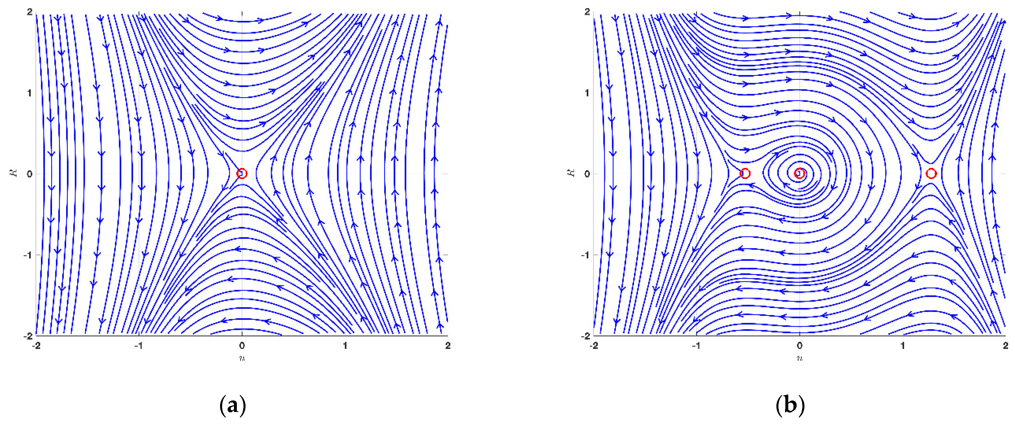
4. Bifurcation Phenomena

The bifurcation theory along with the phase portrait analysis method are going to be used to investigate KdVE and JMHE in the next step.

4.1. Bifurcation Phenomena of KdVE

Through the analysis of Galilean transformation, we modify Equation (16) towards the planar dynamical system in a subsequent way:
d H ζ d ζ = R                                                                     d R ζ d ζ = W 1 H 2 ζ + W 2 H ζ     ,
in which W 1 = α 2 δ ,   W 2 = c ρ δ . The above dynamical system yields the Hamiltonian function:
H 1 H , R = R 2 2 W 1 H 3 3 W 2 H 2 2 = h 1 ,
where h 1 represents the Hamiltonian constant. One could evaluate the equilibrium points 0 ,   0 ,   W 2 W 1 ,   0 by solving the following system:
R = 0                                           W 1 H 2 + W 2 H = 0
Here, the Jacobian measure of the required dynamical system is as follows:
D 1 H , R = 0 1 2 W 1 H + W 2 0 = 2 W 1 H W 2 .
We have from the theory of planar dynamical systems:
  • When D 1 H ,   R is negative, H ,   R represents a saddle point.
  • When D 1 H ,   R is positive, H ,   R represents a center point.
  • When D 1 H ,   R is zero, H ,   R represents a cuspid point.
So, the possible situations with different values of the parameters are provided below.
Circumstance 1: W 1 < 0 and W 2 < 0
In Figure 2a, we observe that the equilibrium points 0 ,   0 and 1 ,   0 for the parameters α = 2 ,   δ = 1 ,   c = 1 ,   ρ = 2 are the center point and the saddle point, individually. Here, red circle are the equilibrium points.
Circumstance 2: W 1 > 0 and W 2 < 0
In Figure 2b, we examine that the equilibrium points 0 ,   0 and 1 ,   0 for the parameters α = 2 ,   δ = 1 ,   c = 1 ,   ρ = 2 appear the center point and the saddle point, correspondingly. Here, red circle are the equilibrium points.

4.2. Bifurcation Phenomena of JMHE
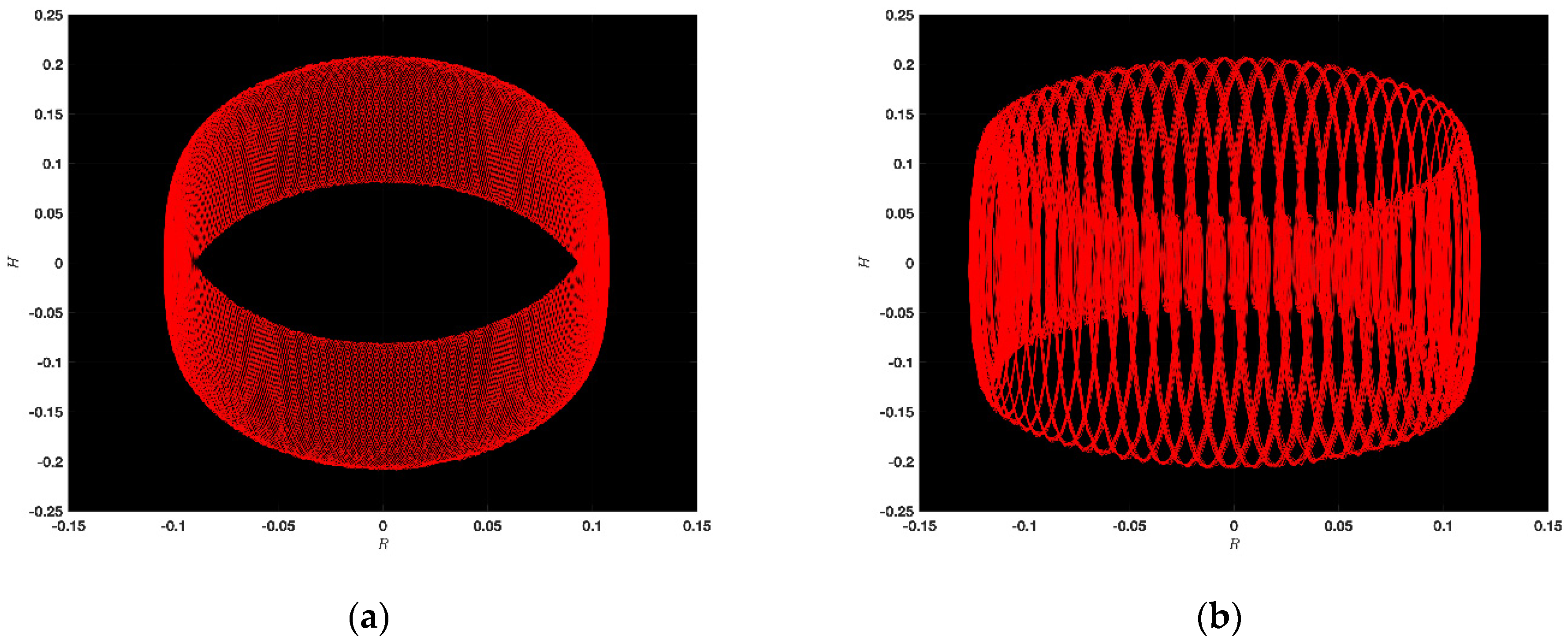
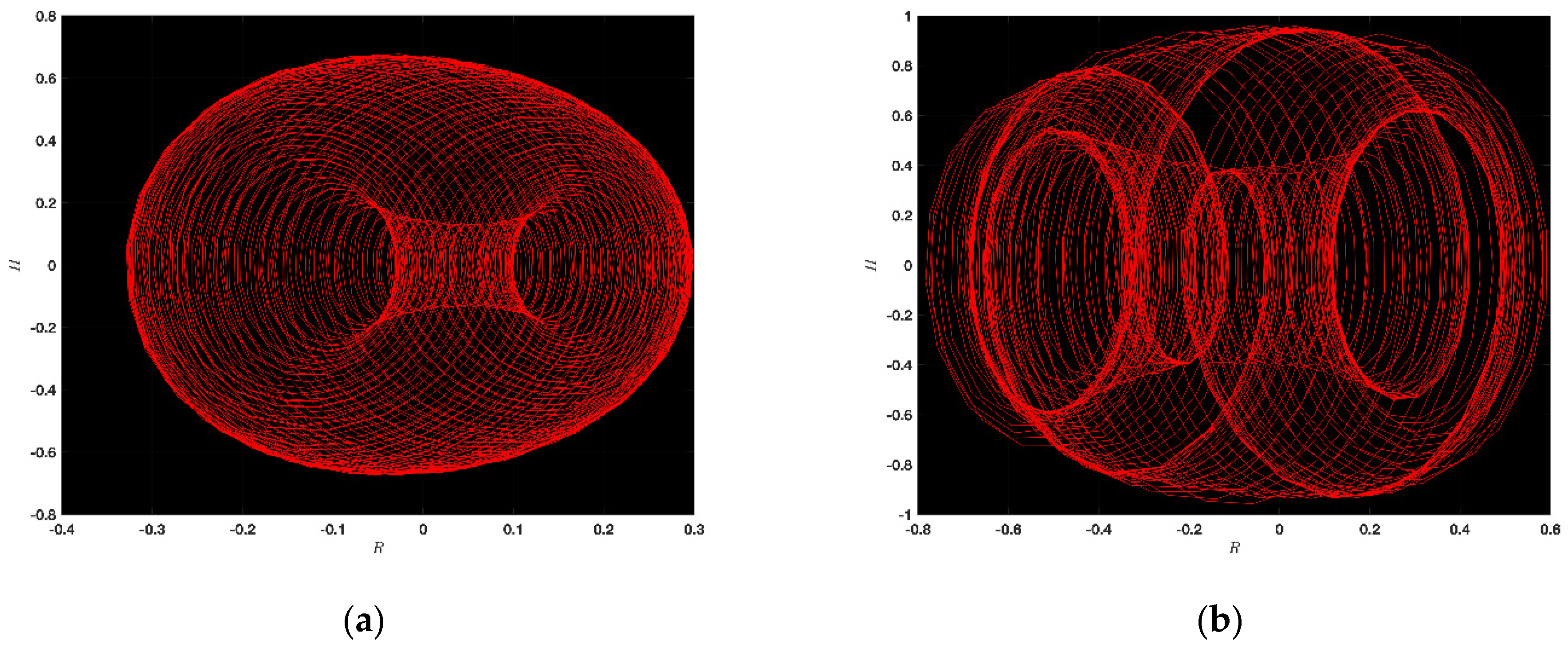
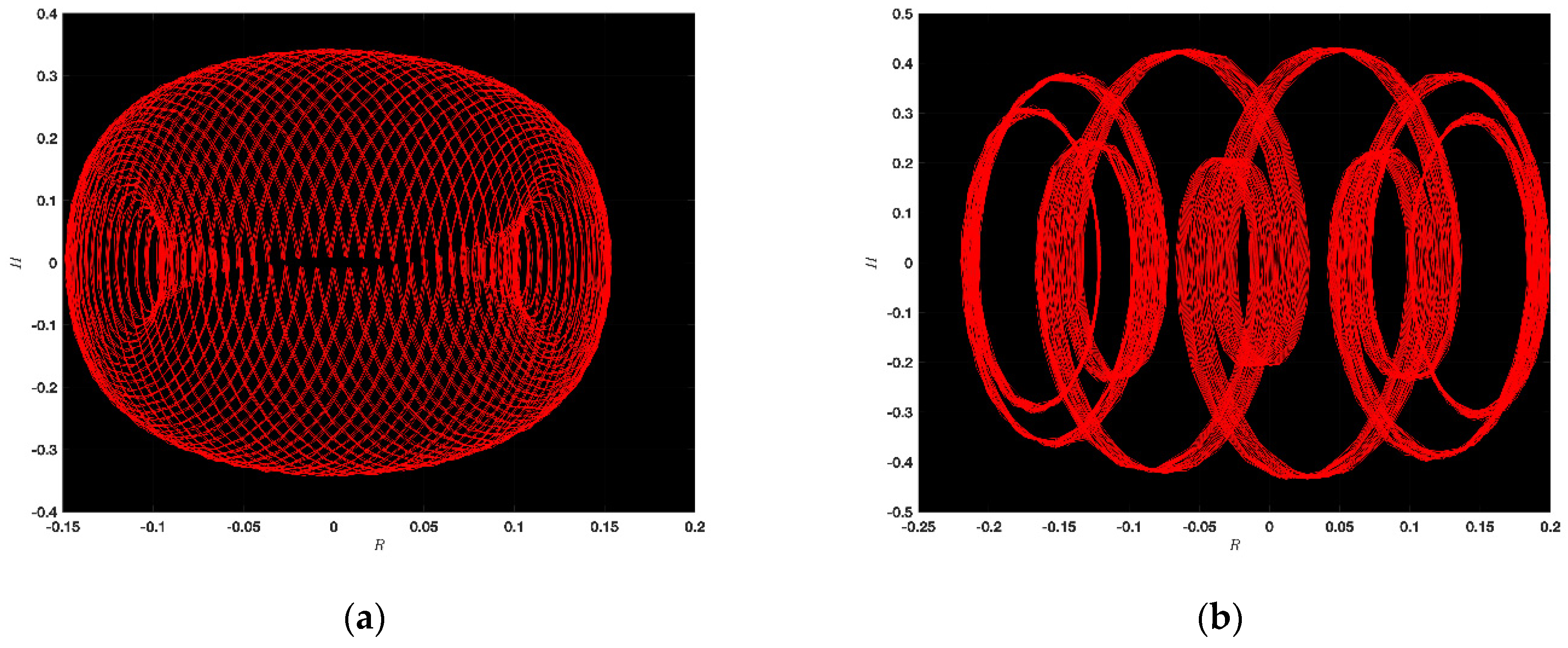
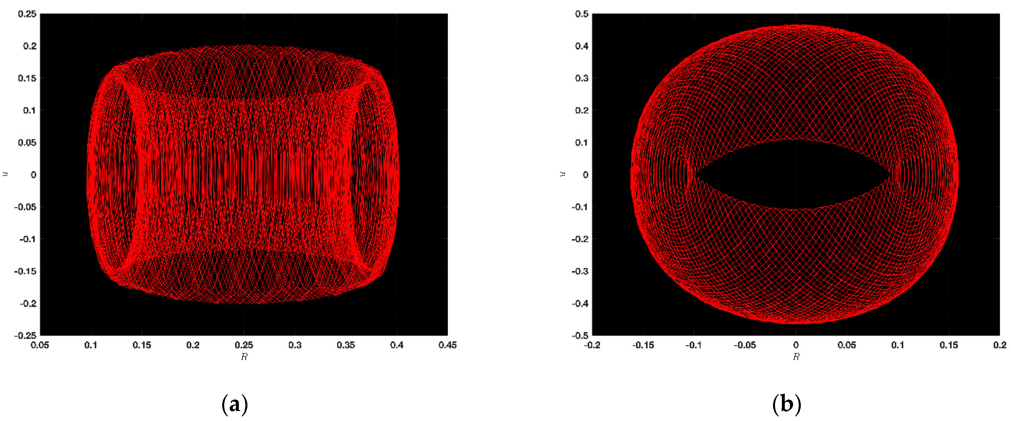
Here, we implement the Galilean transformation to Equation (35) that might supply us with a subsequent planer dynamical system:
d u ζ d ζ = R                                                                                                       d R ζ d ζ = 2 u 3 ζ 3 2   u 2 ζ + W 3 u ζ   ,
wherein W 3 = 16 c + 3 4 . Now, the Hamiltonian function of the dynamical system is of the following form:
H 2 u , R = R 2 2 u 4 2 + u 3 2 W 3 u 2 2 = h 2 ,
wherein h 2 stands for the Hamiltonian constant. So, the equilibrium points of the dynamical system,
R = 0 2 u 3 3 2   u 2 + W 3 u = 0 ,
are 0 ,   0 ,   3 + 9 32 W 3 8 ,   0 ,   3 9 32 W 3 8 ,   0 . The Jacobian measure can be computed from the system,
D 2 u , R = 0 1 6 u 2 3 u + W 3 0 = 6 u 2 + 3 u W 3
So, the possible circumstances along with miscellaneous parameters are offered below. Currently, one can observe the ensuing findings along with the proper values of the parameters.
Circumstance 1: W 3 > 0
In Figure 3a, we check that the equilibrium point 0 ,   0 for the parameter c = 0.5 shows the saddle point. Here, red circle is the equilibrium point.
Circumstance 2: W 3 < 0
In Figure 3b, we see that the equilibrium point 0 ,   0 shows the center point, and 0.5281 ,   0 as well as 1.2781 ,   0 display the saddle points for c = 0.15 , respectively. Here, red circle are the equilibrium points.

5. Chaotic Feature

Chaos theory originated from the study of deterministic dynamical systems whose behavior is highly sensitive to initial conditions, leading to seemingly random and unpredictable outcomes. We wish to identify the chaotic feature of KdVE and JMHE in this section this work.

5.1. Chaotic Analysis of KdVE

By injecting a perturbed term ξ 1 c o s ξ 2 t having the amplitude   ξ 1 and the frequency   ξ 2 , we discover the possibility of chaotic activity in the emerging system (61) in this part:
d H t d t = R d R t d t = W 1 H 2 t + W 2 H t + ξ 1 c o s ξ 2 t    
In Figure 4a, we assume the value of the parameters α = 1 ,   δ = 0.5 ,   c = 1 ,   ρ = 2 ,   ξ 1 = 1 ,   ξ 2 = π / 2 and the others similarly. Here, we oversee in Figure 4, Figure 5 and Figure 6 that the dynamical system has chaotic features alongside ringlet dynamics, periodic dynamics, and complicated dynamics of the acknowledged system. The aforementioned analysis is potentially useful in modern engineering and mathematical physics [28,29,30,31].

5.2. Chaotic Analysis of JMHE

Addressing the chaotic behavior of Equation (62) is the focus of this portion of the article. Right now, a perturbation term ξ 3 c o s ξ 4 t , together with the magnitude ξ 3 and the frequency ξ 4 , would be augmented to the mentioned system as follows:
d u t d t = R d R t d t = 2 u 3 ζ 3 2   u 2 ζ + W 3 u t + ξ 3 c o s ξ 4 t  
Currently, we select the value of the parameter c = 0.25 ,   ξ 3 = 1 ,   ξ 4 = π / 2 in Figure 7a and the others analogously. We scrutinize the chaotic nature including strange dynamics, limit cycles, and periodic dynamics of the anticipated system in Figure 7, Figure 8 and Figure 9. Mathematical physics as well as innovative engineering would gain much from this assessment [28,29,30,31].

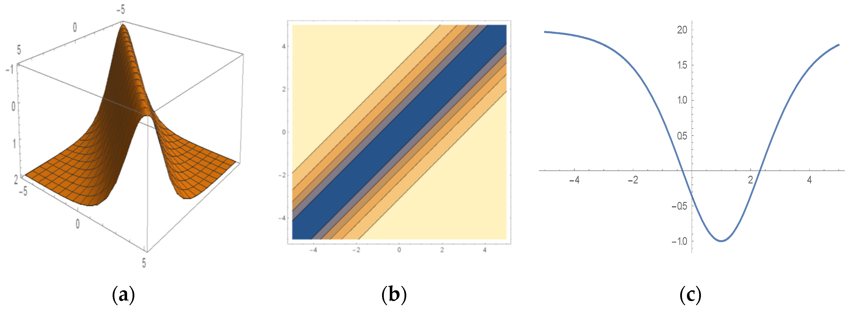
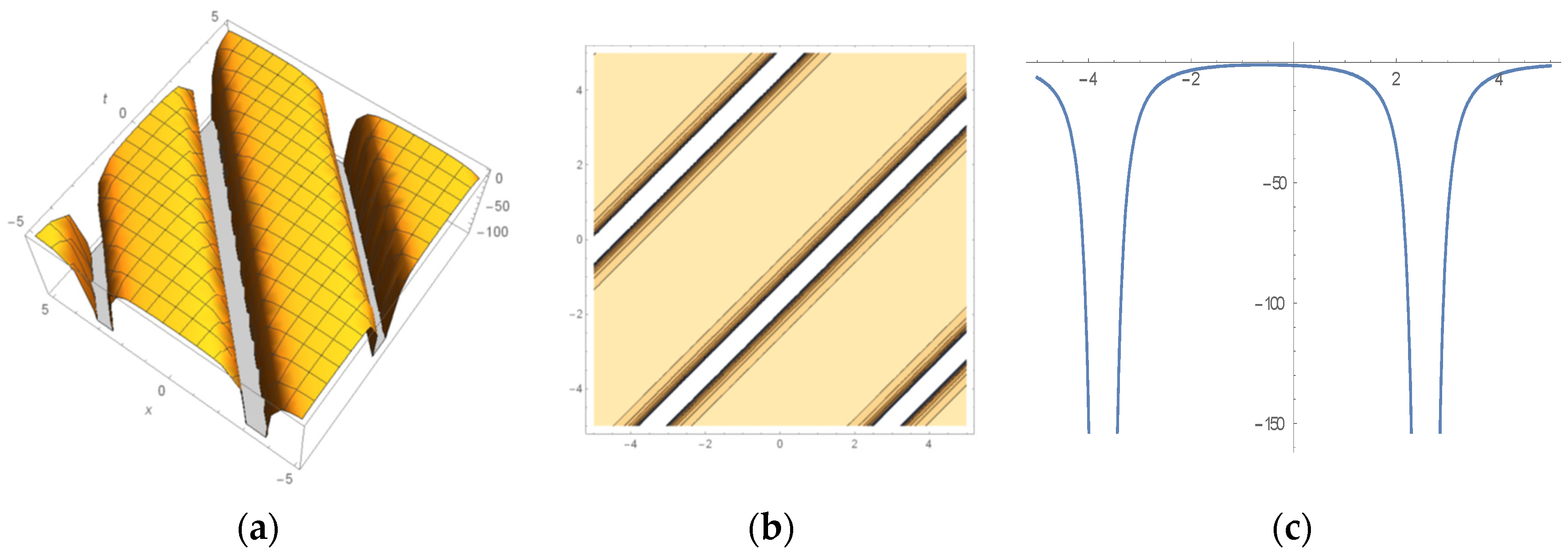
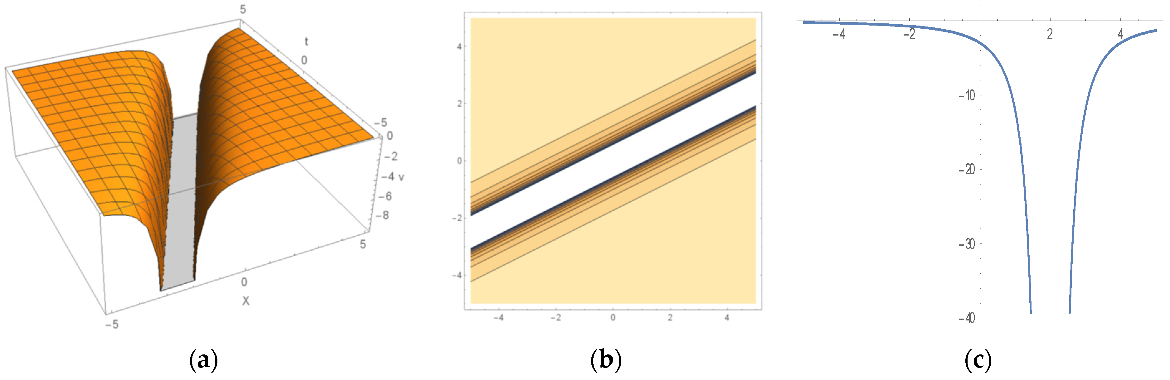
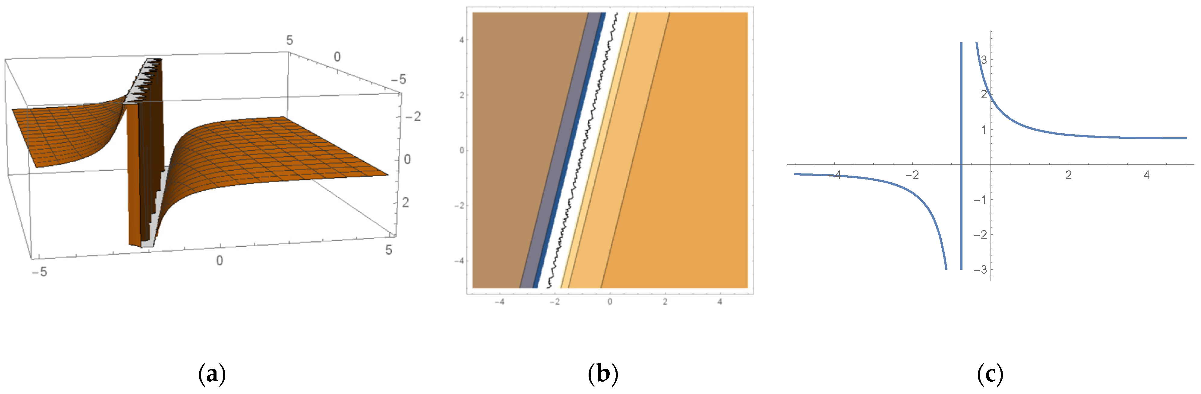
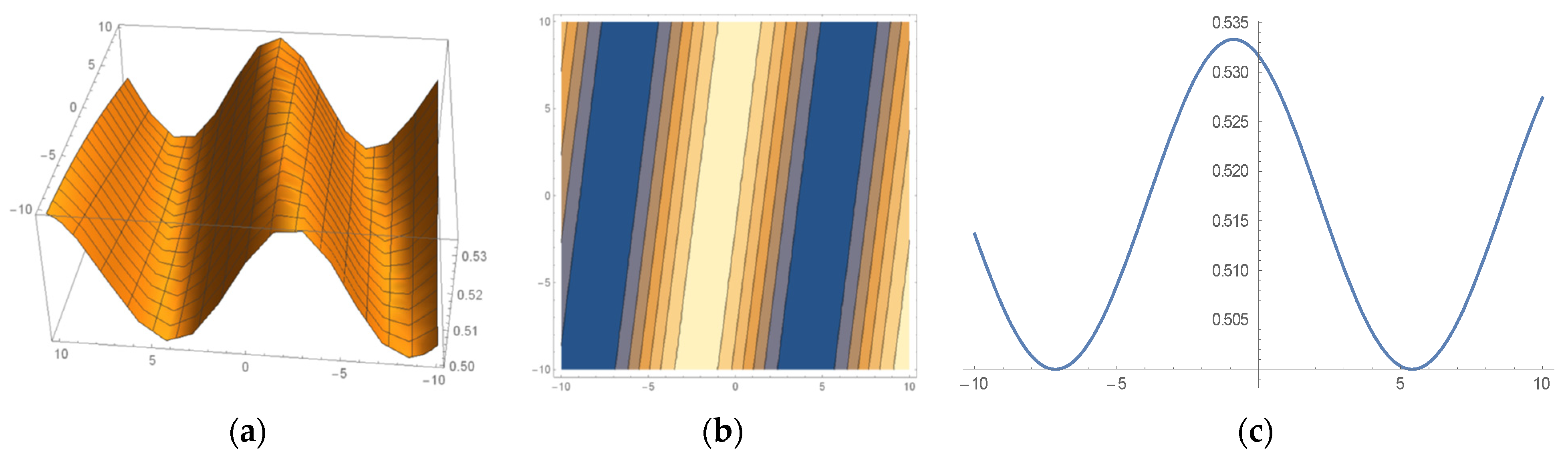
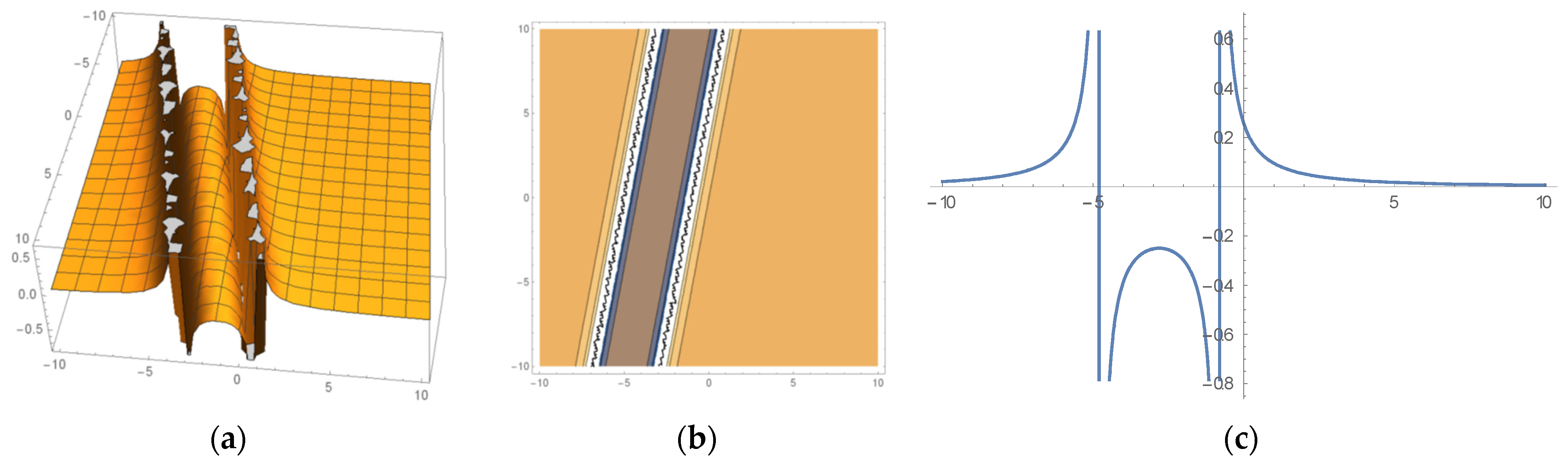
6. Some Important Graphs and Their Discussions

The physical behavior of the problems induced by the Korteweg–de Vries Equation (13) and the Jaulent–Miodek Hierarchy Equation (30) in this study is illustrated with respect to the graphical appearance of some important particular solutions. To interpret the physical phenomena of the two problems, we display the figure of some particular solution in a three-dimensional (3D) shape, a contour shape, and a two-dimensional (2D) shape for the unknown functions H x , t and w t ,   x ,   y . In Figure 10, the kink-shaped soliton is depicted of the particular free surface H x , t solution in Equation (19) for the certain values ρ = 2 , δ = 1 , α = 1 , and λ = 1 . The three-dimensional (3D) and contour shapes of the graphical origination of Equation (21) are represented in Figure 10a and Figure 10b, respectively, while the two-dimensional (2D) shape for t = 1 is displayed in Figure 10c. In Figure 11, the free surface H x , t called the singular periodic soliton for Equation (24) is shown where the three-dimensional (3D) and contour shapes are given in Figure 11a and Figure 11b, respectively, while the certain values ρ = 2 , δ = 1 , α = 1 , and λ = 1 along with a two-dimensional (2D) shape are given in Figure 11c for t = 1 . Furthermore, the surface H x , t for Equation (29) called the singular bell-shaped soliton is depicted in Figure 12a as a three-dimensional (3D) shape; Figure 12b as a contour shape with certain values ρ = 2 , δ = 1 , and α = 1 ; and Figure 12c as a two-dimensional (2D) shape with t = 1 . On the other hand, in Figure 13, the singular soliton is depicted of the analytic function surface w t ,   x ,   y solution in Equation (41) for the certain values λ = 1 , and y = 1 . The three-dimensional (3D) and contour shapes of the graphical origination of Equation (41) are represented in Figure 13a and Figure 13b, respectively, while a two-dimensional (2D) shape for t = 1 is displayed in Figure 13c. In Figure 14, the surface w t ,   x ,   y called the periodic kink-shaped soliton for Equation (50) is shown wherein the three-dimensional (3D) and contour shapes are given in Figure 14a and Figure 14b with the certain values q = 1 , λ = 0.25 , E 1 = 1 , and y = 1 , and a two-dimensional (2D) shape is given in Figure 14c for t = 1 . Moreover, the surface w t ,   x ,   y for Equation (60) called the singular kink-shaped soliton is depicted in Figure 15a as a three-dimensional (3D) shape, Figure 15b as a contour shape with a certain value y = 1 , and Figure 15c for a two-dimensional (2D) shape with t = 1 .

7. Conclusions

In this study, we applied the proposed method to estimate very important new different explicit wave solutions of the KdVE and the JMHE and successfully discussed the dynamical behaviors. We obtained many new interesting soliton solutions that can investigate the models associated with numerous problems of the two equations. These obtained solutions that have not been mentioned before by anybody else were formed for the three new distinct sets of parameter values described in the proposed method called the ( G / G , 1 / G   ) -expansion method. The equilibrium points of the pertinent systems have been established through the utilization of bifurcation analysis. Additionally, we noticed chaotic behavior when an external perturbation term was introduced. The obtained new wave solutions of the KdVE are very important for illustrating a variety of interesting nonlinear water wave phenomena. Moreover, the obtained new wave solutions of the JMHE play a big role in analyzing the behavior of dynamical systems in nonlinear physical phenomena. Many new advanced solutions are formed by choosing values of two arbitrary constants E 1 and E 2 along with q = 0 . A few attained solutions are graphically presented by the 3D, 2D, and contour shapes such as periodic, singular periodic, bell, singular bell, kink, and anti-kink traveling wave features.

Author Contributions

Conceptualization, I.A., M.A.C., M.S.A., K.E.-R. and J.R.M.B.; Methodology, I.A., M.A.C., M.S.A. and M.K.; Software, K.E.-R. and M.M.M.; Validation, I.A., M.M.M. and M.K.; Investigation, I.A., M.A.C., M.S.A., K.E.-R. and J.R.M.B.; Writing—original draft, I.A., M.A.C., M.S.A., K.E.-R. and J.R.M.B.; Writing—review and editing, M.M.M. and M.K.; Supervision, M.M.M. and M.K. All authors have read and agreed to the published version of the manuscript.

Funding

This research received no external funding.

Institutional Review Board Statement

I hereby declare that this manuscript is the result of my independent creation under the reviewers’ comments. Except for the quoted contents, this manuscript does not contain any research achievements that have been published or written by other individuals or groups.

Data Availability Statement

All data generated or analyzed during this study are included in this article.

Acknowledgments

The authors would like to acknowledge Deanship of Graduate Studies and Scientific Research, Taif University for funding this work.

Conflicts of Interest

The authors declare no conflicts of interest.

References

  1. Misirliand, E.; Gurefe, Y. Exp-function method for solving nonlinear evolution equations. Math. Comput. Appl. 2011, 16, 258–266. [Google Scholar] [CrossRef]
  2. Moradi, E.; Varasteh, H.; Abdollahzadeh, A.; Mostafaei-Malekshah, M. The Exp-Function Method for Solving Two Dimensional Sine-Bratu Type Equations. Appl. Math. 2014, 5, 1212–1217. [Google Scholar] [CrossRef]
  3. Pandir, Y.; Akturk, T.; Gurefe, Y.; Juya, H. The Modified Exponential Function Method for Beta Time Fractional Biswas-Arshed Equation. Adv. Math. Phys. 2023, 2023, 1091355. [Google Scholar] [CrossRef]
  4. Zahran, E.H.M.; Khater, M.M.A. Modified extended tanh-function method and its applications to the Bogoyavlenskii equation. Appl. Math. Model. 2016, 40, 1769–1775. [Google Scholar] [CrossRef]
  5. El-shamy, O.; El-barkoki, R.; Ahmed, H.M.; Abbas, W.; Samir, I. Exploration of new solitons in optical medium with higher-order dispersive and nonlinear effects via improved modified extended tanh function method. Alex. Eng. J. 2023, 68, 611–618. [Google Scholar] [CrossRef]
  6. Almatrafi, M.B. Solitary Wave Solutions to a Fractional Model Using the Improved Modified Extended Tanh-Function Method. Fractal Fract. 2023, 7, 252. [Google Scholar] [CrossRef]
  7. Ali, A.T. the new generalized Jacobi elliptic function rational expansion method. J. Comput. Appl. Math. 2011, 235, 4117–4127. [Google Scholar] [CrossRef]
  8. Zahranand, E.H.M.; Khater, M.M.A. Extended Jacobian Elliptic Function Expansion Method and Its Applications in Biology. Appl. Math. 2015, 6, 1174–1181. [Google Scholar] [CrossRef]
  9. Ekici, M. Stationary optical solitons with Kudryashov’s quintuple power law nonlinearity by extended Jacobi’s elliptic function expansion. J. Nonlinear Opt. Phys. Mater. 2023, 32, 2350008. [Google Scholar] [CrossRef]
  10. Lu, B. The first integral method for some time fractional differential equations. J. Math. Anal. Appl. 2012, 395, 684–693. [Google Scholar] [CrossRef]
  11. Zayed, E.M.E.; Amer, Y.A. The First Integral Method and its Application for Deriving the Exact Solutions of a Higher-Order Dispersive Cubic-Quintic Nonlinear Schrödinger Equation. Comput. Math. Model. 2016, 27, 80–94. [Google Scholar] [CrossRef]
  12. Javeed, S.; Imran, T.; Ahmad, H.; Tchier, F.; Zhao, Y.H. New soliton solutions of modified (3+1)-D Wazwaz–Benjamin–Bona–Mahony and (2+1)-D cubic Klein–Gordon equations using first integral method. Open Phys. 2023, 21, 20220229. [Google Scholar] [CrossRef]
  13. Abdelsalam, U.M.; Ghazal, M.G.M. Analytical Wave Solutions for Foam and KdV-Burgers Equations Using Extended Homogeneous Balance Method. Mathematics 2019, 7, 729. [Google Scholar] [CrossRef]
  14. Rady, A.S.A.; Osman, E.S.; Khalfallah, M. The homogeneous balance method and its application to the Benjamin-Bona-Mahoney (BBM) equation. Appl. Math. Comput. 2010, 217, 1385–1390. [Google Scholar]
  15. Radha, B.; Duraisamy, C. The homogeneous balance method and its application for finding the exact solutions for nonlinear equations. J. Ambient Intell. Humaniz. Comput. 2021, 12, 6591–6597. [Google Scholar] [CrossRef]
  16. Lassas, M.; Mueller, J.L.; Siltanen, S.; Stahel, A. The Novikov–Veselov equation and the inverse scattering method: II. Computation. Nonlinearity 2012, 25, 1799–1818. [Google Scholar] [CrossRef]
  17. Gao, P.; Dong, H.; Ma, F. Inverse scattering via nonlinear integral equations method for a sound-soft crack with phaseless data. Appl. Math. 2018, 63, 49–165. [Google Scholar] [CrossRef]
  18. Grudsky, S.M.; Kravchenko, V.V.; Torba, S.M. Realization of the inverse scattering transform method for the Korteweg–de Vries equation. Math. Methods Appl. Sci. 2023, 46, 9217–9251. [Google Scholar] [CrossRef]
  19. Triki, H.; Taha, T.R. The sub-ODE method and soliton solutions for a higher order dispersive cubic–quintic nonlinear Schrödinger equation. Chaos Solitons Fractals 2009, 42, 1068–1072. [Google Scholar] [CrossRef]
  20. Rizvi, S.T.R.; Seadawy, A.R.; Nimra; Ali, K.; Aziz, N. Variety of optical soliton solutions via sub-ODE approach to embedded soliton generating model in quadratic nonlinear media. Int. J. Mod. Phys. 2023, 37, 2350137. [Google Scholar] [CrossRef]
  21. Xu, F.; Feng, Q. A Generalized Sub-ODE Method and Applications for Nonlinear Evolution Equations. J. Sci. Res. Rep. 2013, 2, 571–581. [Google Scholar] [CrossRef]
  22. Cheng, C.; Jiang, Y.L. Lie group analysis method for two classes of fractional partial differential equations. Commun. Nonlinear Sci. Numer. Simul. 2015, 26, 24–35. [Google Scholar] [CrossRef]
  23. Du, X.X.; Tian, B.; Wu, X.Y.; Yin, H.M.; Zhang, C.R. Lie group analysis, analytic solutions and conservation laws of the (3 + 1)-dimensional Zakharov-Kuznetsov-Burgers equation in a collisionless magnetized electron-positron-ion plasma. Eur. Phys. J. Plus 2018, 133, 378. [Google Scholar] [CrossRef]
  24. Bhatti, M.M.; Jun, S.; Khalique, C.M.; Shahid, A.; Fasheng, L.; Mohamed, M.S. Lie group analysis and robust computational approach to examine mass transport process using Jeffrey fluid model. Appl. Math. Comput. 2022, 421, 126936. [Google Scholar] [CrossRef]
  25. Paliathanasis, A.; Krishnakumar, K.; Tamizhmani, K.M.; Leach, P.G.L. Lie Symmetry Analysis of the Black-Scholes-Merton Model for European Options with Stochastic Volatility. Mathematics 2016, 4, 28. [Google Scholar] [CrossRef]
  26. Feng, Y.; Yu, J. Lie symmetry analysis of fractional ordinary differential equation with neutral delay. AIMS Math. 2021, 6, 3592–3605. [Google Scholar] [CrossRef]
  27. Mbusi, S.O.; Adem, A.R.; Muatjetjeja, B. Lie symmetry analysis, multiple exp-function method and conservation laws for the (2+1)-dimensional Boussinesq equation. Opt. Quantum Electron. 2024, 56, 670. [Google Scholar] [CrossRef]
  28. Chahlaoui, Y.; Ali, A.; Ahmad, J.; Javed, S. Dynamical behavior of chaos, bifurcation analysis and soliton solutions to a Konno-Onno model. PLoS ONE 2023, 18, e0291197. [Google Scholar] [CrossRef] [PubMed]
  29. Tang, L. Bifurcation studies, chaotic pattern, phase diagrams and multiple optical solitons for the (2 + 1)-dimensional stochastic coupled nonlinear Schrödinger system with multiplicative white noise via Itô calculus. Results Phys. 2023, 52, 106765. [Google Scholar] [CrossRef]
  30. Rafiq, M.H.; Raza, N.; Jhangeer, A. Dynamic study of bifurcation, chaotic behavior and multi-soliton profiles for the system of shallow water wave equations with their stability. Chaos Solitons Fractals 2023, 171, 113436. [Google Scholar] [CrossRef]
  31. Rahman, M.U.; Sun, M.; Boulaaras, S.; Baleanu, D. Bifurcations, chaotic behavior, sensitivity analysis, and various soliton solutions for the extended nonlinear Schrödinger equation. Bound. Value Probl. 2024, 2024, 15. [Google Scholar] [CrossRef]
  32. Rizvi, S.T.R.; Seadawy, A.R.; Ashraf, F.; Younis, M.; Iqbal, H.; Baleanu, D. Lump and Interaction solutions of a geophysical Korteweg–de Vries equation. Results Phys. 2020, 19, 103661. [Google Scholar] [CrossRef]
  33. Khalique, C.M. Closed-form solutions and conservation laws of ageneralized Hirota–Satsuma coupled KdV system of fluid mechanics. Open Phys. 2021, 19, 18–25. [Google Scholar] [CrossRef]
  34. Karakoc, S.B.G.; Ali, K.K.; Mehanna, M.S. Exact Traveling Wave Solutions of the Schamel-KdV Equation with Two Different Methods. Univers. J. Math. Appl. 2023, 6, 65–75. [Google Scholar] [CrossRef]
  35. Hou, S.; Zhang, R.; Zhang, Z.; Yang, L. On the Quartic Korteweg–de Vries hierarchy of nonlinear Rossby waves and its dynamics. Wave Motion 2024, 124, 103249. [Google Scholar] [CrossRef]
  36. Prins, J.; Wahls, S. Soliton Phase Shift Calculation for the Korteweg–De Vries Equation. IEEE Access 2019, 7, 122914–122930. [Google Scholar] [CrossRef]
  37. Naowarat, S.; Saifullah, S.; Sen, M.D.L. Periodic, Singular and Dark Solitons of a Generalized Geophysical KdV Equation by Using the Tanh-Coth Method. Symmetry 2023, 15, 135. [Google Scholar] [CrossRef]
  38. Saifullah, S.; Fatima, N.; Abdelmohsen, S.A.M.; Alanazi, M.M.; Ahmad, S.; Baleanu, D. Analysis of a conformable generalized geophysical KdV equation with Coriolis effect. Alex. Eng. J. 2023, 73, 651–663. [Google Scholar] [CrossRef]
  39. Li, J.; Li, X.; Zhang, W. Research on Traveling Wave Solutions for a Class of (3+1)-Dimensional Nonlinear Equation. J. Appl. Anal. Comput. 2017, 7, 841–856. [Google Scholar]
  40. Akkilic, A.N.; Sulaiman, T.A.; Shakir, A.P.; Ismael, H.F.; Bulut, H.; Shah, N.A.; Ali, M.R. Jaulent–Miodek evolution equation: Analytical methods and various solutions. Results Phys. 2023, 47, 106351. [Google Scholar] [CrossRef]
  41. Sadat, R.; Kassem, M. Explicit Solutions for the (2 + 1)-Dimensional Jaulent–Miodek Equation Using the Integrating Factors Method in an Unbounded Domain. Math. Comput. Appl. 2018, 23, 15. [Google Scholar] [CrossRef]
  42. Ige, O.E.; Oderinu, R.A.; Elzaki, T.M. Numerical Simulation of the Nonlinear Coupled Jaulent-Miodek Equation by Elzaki Transform-Adomain Polynomial Method. Adv. Math. Sci. J. 2020, 9, 10335–10355. [Google Scholar] [CrossRef]
  43. Cakicioglu, H.; Ozisik, M.; Secer, A.; Bayram, M. Kink Soliton Dynamic of the (2+1)-Dimensional Integro-Differential Jaulent–Miodek Equation via a Couple of Integration Techniques. Symmetry 2023, 15, 1090. [Google Scholar] [CrossRef]
  44. Ma, H.C.; Deng, A.P.; Yu, Y.D. Lie Symmetry Group of (2 + 1)-Dimensional Jaulent-Miodek Equation. Therm. Sci. 2014, 18, 1547–1552. [Google Scholar] [CrossRef]
  45. Chowdhury, M.A.; Miah, M.M.; Iqbal, M.A.; Alshehri, H.M.; Baleanu, D.; Osman, M.S. Advanced exact solutions to the nano-ionic currents equation through MTs and the soliton equation containing the RLC transmission line. Eur. Phys. J. Plus 2023, 138, 502. [Google Scholar] [CrossRef]
  46. Li, L.X.; Li, E.Q.; Wang, M.L. The (G′/G, 1/G)-expansion method and its application to travelling wave solutions of the Zakharov equations. Appl. Math. A J. Chin. Univ. 2010, 25, 454–462. [Google Scholar] [CrossRef]
  47. Zayed, E.M.E.; Alurrfi, K.A.E. The (G′/G, 1/G)-Expansion Method and Its Applications to Find the Exact Solutions of Nonlinear PDEs for Nanobiosciences. Math. Probl. Eng. 2014, 2014, 521712. [Google Scholar] [CrossRef]
  48. Miah, M.M.; Ali, H.M.S.; Akbar, M.A.; Wazwaz, A.M. Some applications of the (G′/G, 1/G)-expansion method to find new exact solutions of NLEEs. Eur. Phys. J. Plus 2017, 132, 252. [Google Scholar] [CrossRef]
  49. Kaplan, M.; Bekir, A.; Akbulut, A. A generalized Kudryashov method to some nonlinear evolution equations in mathematical physics. Nonlinear Dyn. 2016, 85, 2843–2850. [Google Scholar] [CrossRef]
Figure 1. Flowchart of our research work.
Mathematics 12 02053 g001
Figure 2. Bifurcation phenomena of the expected dynamical system for various situation of W 1 and W 2 , (a) α = 2 ,   δ = 1 ,   c = 1 ,   ρ = 2 and (b) α = 2 ,   δ = 1 ,   c = 1 ,   ρ = 2 .
Mathematics 12 02053 g002
Figure 3. Bifurcation phenomena of the mentioned dynamical system by means of diverse situations of W 3 , (a) c = 0.5 and (b) c = 0.15 .
Mathematics 12 02053 g003
Figure 4. The chaotic feature of the stated system has several values of the parameters with ξ 2 = π / 2 , (a) α = 1 ,   δ = 0.5 ,   c = 1 ,   ρ = 2 ,   ξ 1 = 1 and (b) α = 2 ,   δ = 2 ,   c = 1 ,   ρ = 2 ,   ξ 1 = 2 .
Mathematics 12 02053 g004
Figure 5. The chaotic feature of the offered system has several values of the parameters with ξ 2 = π , (a) α = 1 ,   δ = 0.5 ,   c = 1 ,   ρ = 2 ,   ξ 1 = 1 and (b) α = 2 ,   δ = 2 ,   c = 1 ,   ρ = 2 ,   ξ 1 = 2 .
Mathematics 12 02053 g005
Figure 6. The chaotic feature of the reported system has several values of the parameters with ξ 2 = 2 π , (a) α = 1 ,   δ = 0.5 ,   c = 1 ,   ρ = 2 ,   ξ 1 = 1 and (b) α = 2 ,   δ = 2 ,   c = 1 ,   ρ = 2 ,   ξ 1 = 2 .
Mathematics 12 02053 g006
Figure 7. The chaotic nature of the proposed system with distinct value of the parameter containing ξ 4 = π / 2 , (a) c = 0.25 ,     ξ 3 = 1 and (b) c = 1 ,     ξ 3 = 1 .
Mathematics 12 02053 g007
Figure 8. The chaotic nature of the recommended system with distinct value of the parameter containing ξ 4 = π , (a) c = 0.25 ,     ξ 3 = 1 and (b) c = 1 ,     ξ 3 = 1 .
Mathematics 12 02053 g008
Figure 9. The chaotic nature of the suggested system with distinct value of the parameter containing ξ 4 = 2 π , (a) c = 0.25 ,     ξ 3 = 1 and (b) c = 1 ,     ξ 3 = 1 .
Mathematics 12 02053 g009
Figure 10. The kink-shaped soliton: 3D shape in (a), the contour shape in (b) for x ,   t = [ 5 ,   5 ] , and 2D surface in (c) for x = [ 5 ,   5 ] , t = 1 for the solution of Equation (19).
Mathematics 12 02053 g010
Figure 11. The singular periodic soliton: 3D in (a), the contour shape in (b) for x ,   t = [ 5 ,   5 ] , and 2D surface in (c) for x = [ 5 ,   5 ] , t = 1 for the solution of Equation (24).
Mathematics 12 02053 g011
Figure 12. The singular bell-shaped soliton: 3D in (a), the contour shape in (b) for x ,   t = [ 5 ,   5 ] , and 2D surface in (c) for x = [ 5 ,   5 ] , t = 1 for the solution of Equation (29).
Mathematics 12 02053 g012
Figure 13. The singular soliton: 3D in (a), the contour shape in (b) for x ,   t = [ 5 ,   5 ] , y = 1 , and 2D surface in (c) for x = [ 5 ,   5 ] , y = 1 , t = 1 for the solution of Equation (41).
Mathematics 12 02053 g013
Figure 14. The periodic kink-shaped soliton: 3D in (a), the contour shape in (b) for x ,   t = [ 10 ,   10 ] , y = 1 , and 2D surface in (c) for x = [ 10 ,   10 ] , y = 1 , t = 1 for the solution of Equation (50).
Mathematics 12 02053 g014
Figure 15. The singular kink-shaped soliton: 3D in (a), the contour shape in (b) for x ,   t = [ 10 ,   10 ] , y = 1 , and 2D surface in (c) for x = [ 10 ,   10 ] , y = 1 , t = 1 for the solution of Equation (60).
Mathematics 12 02053 g015
Disclaimer/Publisher’s Note: The statements, opinions and data contained in all publications are solely those of the individual author(s) and contributor(s) and not of MDPI and/or the editor(s). MDPI and/or the editor(s) disclaim responsibility for any injury to people or property resulting from any ideas, methods, instructions or products referred to in the content.

