
Reparameterized Scale Mixture of Rayleigh Distribution Regression Models with Varying Precision

 , , and
Abstract
:1. Introduction
2. An SMR Distribution Parameterized by Its Mean and Precision Parameters
3. RSMR Regression Model
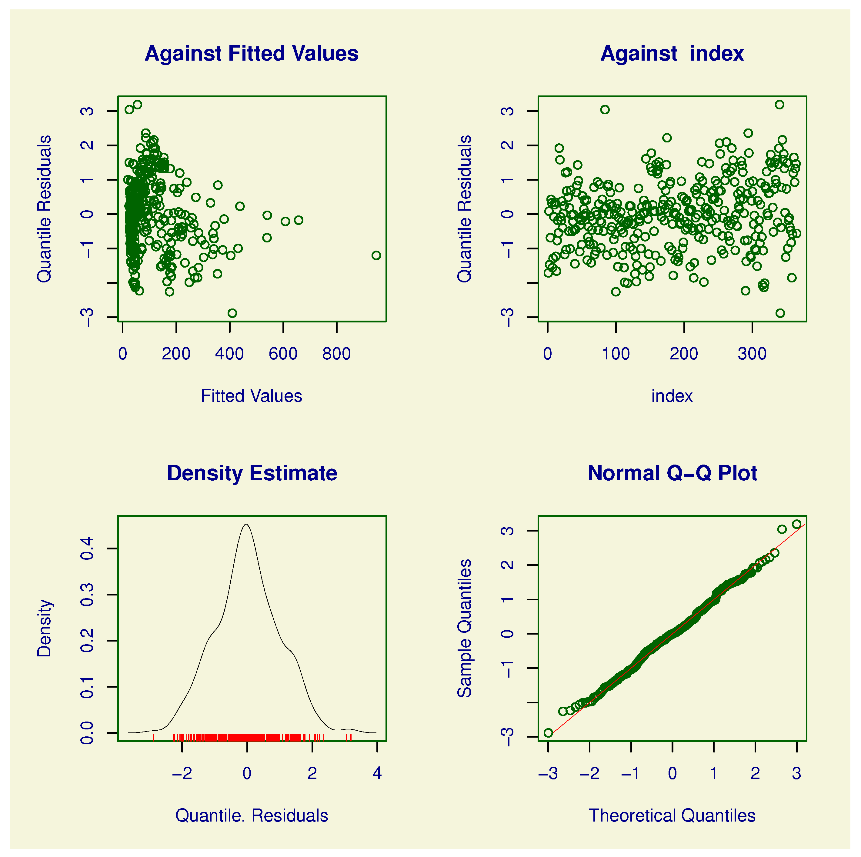
3.1. Residuals
Randomized Quantile Residuals
3.2. Deviance Residuals
4. Simulation Study
5. Real Data Application
5.1. MASS Package
- pH00, pH30, and pH80: pH at depth 0–10, 30–40, and 80–90 cm, respectively;
- e00, e30, and e80: electrical conductivity in mS/cm (0–10 cm), (30–40 cm), and (80–90 cm), respectively;
- c00, c30, and c80: chloride content in ppm (0–10 cm), (30–40 cm), and (80–90 cm), respectively.
5.2. Gamlss Package: Fit
6. Conclusions
Author Contributions
Funding
Data Availability Statement
Conflicts of Interest
Appendix A. Simulated Results

| se | RMSE | % Cov. | ||||||
|---|---|---|---|---|---|---|---|---|
| −0.3 | 0.5 | 0 | 0.7 | −0.3380 | 0.0927 | 0.0862 | 0.91 | |
| 0.4797 | 0.0916 | 0.0762 | 0.93 | |||||
| −0.0009 | 0.0942 | 0.0840 | 0.91 | |||||
| 1.7051 | 1.1172 | 1.0119 | 1.00 | |||||
| −0.3245 | 0.0694 | 0.0611 | 0.92 | |||||
| 0.4935 | 0.0602 | 0.0489 | 0.94 | |||||
| 0.0025 | 0.0660 | 0.0560 | 0.92 | |||||
| 1.2640 | 0.6573 | 0.5781 | 0.99 | |||||
| −0.3125 | 0.0517 | 0.0411 | 0.93 | |||||
| 0.4999 | 0.0468 | 0.0376 | 0.94 | |||||
| −0.0013 | 0.0483 | 0.0402 | 0.94 | |||||
| 0.9655 | 0.4306 | 0.3303 | 0.94 | |||||
| −0.3 | 0.25 | −0.3 | 0.7 | −0.3419 | 0.0979 | 0.0917 | 0.89 | |
| 0.2543 | 0.1082 | 0.0993 | 0.90 | |||||
| −0.2969 | 0.0933 | 0.0816 | 0.92 | |||||
| 1.6772 | 1.1181 | 0.9840 | 1.00 | |||||
| −0.3280 | 0.0702 | 0.0624 | 0.91 | |||||
| 0.2478 | 0.0718 | 0.0589 | 0.94 | |||||
| −0.2965 | 0.0569 | 0.0475 | 0.94 | |||||
| 1.2624 | 0.6587 | 0.5760 | 0.99 | |||||
| −0.3134 | 0.0520 | 0.0436 | 0.94 | |||||
| 0.2545 | 0.0536 | 0.0424 | 0.95 | |||||
| −0.2975 | 0.0485 | 0.0391 | 0.95 | |||||
| 0.9610 | 0.4325 | 0.3256 | 0.94 | |||||
| −0.3 | 0 | 0 | 0.7 | −0.3366 | 0.0922 | 0.0875 | 0.90 | |
| 0.0016 | 0.0877 | 0.0756 | 0.93 | |||||
| 0.0047 | 0.0868 | 0.0774 | 0.92 | |||||
| 1.6621 | 1.0891 | 0.9689 | 1.00 | |||||
| −0.3235 | 0.0696 | 0.0601 | 0.91 | |||||
| 0.0002 | 0.0686 | 0.0591 | 0.93 | |||||
| −0.0009 | 0.0641 | 0.0546 | 0.93 | |||||
| 1.2229 | 0.6447 | 0.5367 | 0.99 | |||||
| −0.3138 | 0.0518 | 0.0422 | 0.94 | |||||
| −0.0006 | 0.0476 | 0.0379 | 0.94 | |||||
| −0.0045 | 0.0523 | 0.0414 | 0.93 | |||||
| 0.9591 | 0.4316 | 0.3241 | 0.95 | |||||
| se | RMSE | % Cov. | ||||||
|---|---|---|---|---|---|---|---|---|
| −0.2 | 0.5 | 0.8 | 1.3 | −0.2133 | 0.0878 | 0.0778 | 0.92 | |
| 0.4929 | 0.0921 | 0.0760 | 0.93 | |||||
| 0.7743 | 0.0936 | 0.0745 | 0.94 | |||||
| 2.0817 | 1.3548 | 0.8630 | 1.00 | |||||
| −0.1926 | 0.0667 | 0.0552 | 0.94 | |||||
| 0.4628 | 0.0763 | 0.0622 | 0.93 | |||||
| 0.7334 | 0.0608 | 0.0737 | 0.81 | |||||
| 1.7633 | 0.9083 | 0.7928 | 0.99 | |||||
| −0.1967 | 0.0489 | 0.0396 | 0.95 | |||||
| 0.4858 | 0.0459 | 0.0319 | 0.95 | |||||
| 0.7709 | 0.0464 | 0.0426 | 0.91 | |||||
| 1.3095 | 0.5066 | 0.4513 | 0.99 | |||||
| −0.2 | 0.25 | 0.8 | 1.3 | −0.2295 | 0.0875 | 0.0796 | 0.91 | |
| 0.2239 | 0.0965 | 0.0808 | 0.94 | |||||
| 0.7565 | 0.0983 | 0.0844 | 0.93 | |||||
| 2.0389 | 1.3051 | 0.8243 | 1.00 | |||||
| −0.2055 | 0.0657 | 0.0532 | 0.95 | |||||
| 0.2499 | 0.0642 | 0.0512 | 0.96 | |||||
| 0.7775 | 0.0625 | 0.0503 | 0.95 | |||||
| 1.6055 | 0.7559 | 0.5537 | 1.00 | |||||
| −0.1997 | 0.0474 | 0.0375 | 0.95 | |||||
| 0.2501 | 0.0497 | 0.0399 | 0.95 | |||||
| 0.7879 | 0.0505 | 0.0413 | 0.95 | |||||
| 1.3712 | 0.4505 | 0.3176 | 0.99 | |||||
| −0.2 | 0 | 0.8 | 1.3 | −0.2173 | 0.0893 | 0.0756 | 0.94 | |
| −0.0045 | 0.0953 | 0.0819 | 0.94 | |||||
| 0.7957 | 0.0967 | 0.0788 | 0.94 | |||||
| 1.9084 | 1.2111 | 0.6987 | 1.00 | |||||
| −0.2069 | 0.0653 | 0.0549 | 0.93 | |||||
| 0.0049 | 0.0696 | 0.0561 | 0.95 | |||||
| 0.7879 | 0.0657 | 0.0531 | 0.94 | |||||
| 1.6471 | 0.7601 | 0.5623 | 1.00 | |||||
| −0.1977 | 0.0484 | 0.0376 | 0.95 | |||||
| 0.0019 | 0.0474 | 0.0368 | 0.96 | |||||
| 0.7794 | 0.0425 | 0.0365 | 0.94 | |||||
| 1.3764 | 0.4707 | 0.3918 | 0.99 | |||||
| −0.2 | 0.5 | −0.3 | 1.3 | −0.2155 | 0.0895 | 0.0759 | 0.93 | |
| 0.4868 | 0.0869 | 0.0692 | 0.95 | |||||
| −0.2979 | 0.0937 | 0.0800 | 0.92 | |||||
| 1.9269 | 1.2313 | 0.7285 | 1.00 | |||||
| −0.2105 | 0.0648 | 0.0546 | 0.94 | |||||
| 0.4968 | 0.0641 | 0.0526 | 0.95 | |||||
| −0.2969 | 0.0578 | 0.0468 | 0.95 | |||||
| 1.6587 | 0.7587 | 0.5527 | 1.00 | |||||
| −0.2018 | 0.0473 | 0.0382 | 0.93 | |||||
| 0.5003 | 0.0494 | 0.0404 | 0.94 | |||||
| −0.3009 | 0.0463 | 0.0375 | 0.94 | |||||
| 1.4277 | 0.4620 | 0.3456 | 0.99 | |||||
| −0.2 | 0.5 | 0 | 1.3 | −0.2196 | 0.0926 | 0.0782 | 0.93 | |
| 0.4987 | 0.0939 | 0.0784 | 0.95 | |||||
| 0.0048 | 0.0834 | 0.0685 | 0.94 | |||||
| 1.8430 | 1.1669 | 0.6403 | 1.00 | |||||
| −0.2071 | 0.0649 | 0.0525 | 0.94 | |||||
| 0.4943 | 0.0682 | 0.0563 | 0.94 | |||||
| −0.0048 | 0.0578 | 0.0499 | 0.93 | |||||
| 1.6330 | 0.7588 | 0.5319 | 1.00 | |||||
| −0.2017 | 0.0471 | 0.0387 | 0.94 | |||||
| 0.5005 | 0.0471 | 0.0384 | 0.94 | |||||
| −0.0014 | 0.0464 | 0.0353 | 0.95 | |||||
| 1.4435 | 0.4633 | 0.3758 | 0.99 | |||||
| −0.2 | 0.25 | −0.3 | 1.3 | −0.2135 | 0.0888 | 0.0746 | 0.93 | |
| 0.2459 | 0.1039 | 0.0903 | 0.92 | |||||
| −0.2973 | 0.0908 | 0.0717 | 0.94 | |||||
| 1.8519 | 1.1839 | 0.6639 | 1.00 | |||||
| −0.2047 | 0.0657 | 0.0544 | 0.95 | |||||
| 0.2509 | 0.0661 | 0.0543 | 0.94 | |||||
| −0.3008 | 0.0609 | 0.0509 | 0.93 | |||||
| 1.5863 | 0.7245 | 0.5005 | 1.00 | |||||
| −0.2051 | 0.0473 | 0.0385 | 0.95 | |||||
| 0.2502 | 0.0457 | 0.0367 | 0.95 | |||||
| -0.3002 | 0.0449 | 0.0351 | 0.94 | |||||
| 1.4318 | 0.4623 | 0.3612 | 0.99 | |||||
| se | RMSE | % Cov. | ||||||
|---|---|---|---|---|---|---|---|---|
| −0.2 | 0 | 0 | 1.3 | −0.2158 | 0.0889 | 0.0741 | 0.94 | |
| 0.0071 | 0.0949 | 0.0786 | 0.94 | |||||
| 0.0041 | 0.0836 | 0.0688 | 0.94 | |||||
| 1.8456 | 1.1793 | 0.6392 | 1.00 | |||||
| −0.2091 | 0.0651 | 0.0547 | 0.93 | |||||
| 0.0017 | 0.0646 | 0.0550 | 0.93 | |||||
| 0.0018 | 0.0667 | 0.0549 | 0.95 | |||||
| 1.6153 | 0.7492 | 0.5129 | 1.00 | |||||
| −0.2037 | 0.0473 | 0.0382 | 0.95 | |||||
| 0.0006 | 0.0470 | 0.0401 | 0.94 | |||||
| 0.0001 | 0.0461 | 0.0380 | 0.94 | |||||
| 1.4376 | 0.4622 | 0.3549 | 0.99 | |||||
| 0.1 | −0.9 | 0.4 | 2.3 | 0.0816 | 0.0809 | 0.0703 | 0.92 | |
| −0.8572 | 0.0829 | 0.0705 | 0.94 | |||||
| 0.3909 | 0.0771 | 0.0613 | 0.95 | |||||
| 3.1047 | 2.1269 | 1.1778 | 0.99 | |||||
| 0.0928 | 0.0561 | 0.0477 | 0.93 | |||||
| −0.8727 | 0.0581 | 0.0485 | 0.94 | |||||
| 0.3989 | 0.0536 | 0.0448 | 0.93 | |||||
| 3.3279 | 1.9031 | 1.2772 | 0.98 | |||||
| 0.0969 | 0.0389 | 0.0318 | 0.94 | |||||
| −0.8789 | 0.0411 | 0.0384 | 0.92 | |||||
| 0.3855 | 0.0415 | 0.0363 | 0.92 | |||||
| 3.3714 | 1.5050 | 1.2099 | 0.99 | |||||
| se | RMSE | % Cov. | ||||||
|---|---|---|---|---|---|---|---|---|
| 0.1 | 0.25 | 0.4 | 2.3 | 0.0889 | 0.0840 | 0.0672 | 0.95 | |
| 0.2455 | 0.0762 | 0.0623 | 0.93 | |||||
| 0.3959 | 0.0708 | 0.0566 | 0.96 | |||||
| 2.3443 | 1.4810 | 0.6362 | 1.00 | |||||
| 0.0931 | 0.0594 | 0.0465 | 0.96 | |||||
| 0.2513 | 0.0559 | 0.0452 | 0.95 | |||||
| 0.4040 | 0.0619 | 0.0489 | 0.95 | |||||
| 2.3964 | 1.1167 | 0.5963 | 0.98 | |||||
| 0.0996 | 0.0409 | 0.0339 | 0.94 | |||||
| 0.2509 | 0.0404 | 0.0326 | 0.95 | |||||
| 0.3978 | 0.0375 | 0.0298 | 0.96 | |||||
| 2.4670 | 0.7939 | 0.4702 | 0.98 | |||||
| 0.1 | 0 | 0.4 | 2.3 | 0.0911 | 0.0849 | 0.0668 | 0.95 | |
| 0.0005 | 0.0832 | 0.0638 | 0.96 | |||||
| 0.4035 | 0.0883 | 0.0703 | 0.95 | |||||
| 2.3143 | 1.4615 | 0.6092 | 1.00 | |||||
| 0.0944 | 0.0594 | 0.0485 | 0.94 | |||||
| −0.0004 | 0.0627 | 0.0503 | 0.94 | |||||
| 0.3993 | 0.0633 | 0.0509 | 0.95 | |||||
| 2.3285 | 1.0408 | 0.5454 | 0.98 | |||||
| 0.0980 | 0.0415 | 0.0329 | 0.95 | |||||
| −0.0014 | 0.0398 | 0.0323 | 0.94 | |||||
| 0.3972 | 0.0395 | 0.0323 | 0.95 | |||||
| 2.3969 | 0.7638 | 0.4708 | 0.98 | |||||
| 0.1 | −0.9 | −0.3 | 2.3 | 0.0874 | 0.0854 | 0.0650 | 0.96 | |
| −0.8848 | 0.1055 | 0.0809 | 0.96 | |||||
| −0.2998 | 0.0889 | 0.0712 | 0.96 | |||||
| 2.4723 | 1.5877 | 0.7407 | 1.00 | |||||
| 0.0935 | 0.0559 | 0.0465 | 0.94 | |||||
| −0.8674 | 0.0576 | 0.0525 | 0.91 | |||||
| −0.2889 | 0.0520 | 0.0422 | 0.94 | |||||
| 3.2666 | 1.8451 | 1.2295 | 0.98 | |||||
| 0.0945 | 0.0396 | 0.0325 | 0.94 | |||||
| −0.8833 | 0.0435 | 0.0367 | 0.94 | |||||
| −0.2956 | 0.0391 | 0.0322 | 0.95 | |||||
| 2.9612 | 1.1331 | 0.8559 | 0.98 | |||||
| se | RMSE | % Cov. | ||||||
|---|---|---|---|---|---|---|---|---|
| 0.1 | 0 | 2.3 | 0.0872 | 0.0836 | 0.0664 | 0.96 | ||
| −0.9020 | 0.0929 | 0.0709 | 0.95 | |||||
| 0.0050 | 0.0927 | 0.0701 | 0.97 | |||||
| 2.3302 | 1.4452 | 0.6193 | 0.99 | |||||
| 0.0952 | 0.0573 | 0.0451 | 0.95 | |||||
| −0.8897 | 0.0605 | 0.0489 | 0.94 | |||||
| 0.0054 | 0.0673 | 0.0526 | 0.96 | |||||
| 2.7286 | 1.3207 | 0.7811 | 0.99 | |||||
| 0.0955 | 0.0395 | 0.0330 | 0.93 | |||||
| −0.8659 | 0.0422 | 0.0446 | 0.88 | |||||
| −0.0024 | 0.0456 | 0.0338 | 0.94 | |||||
| 3.2724 | 1.3848 | 1.1547 | 0.98 | |||||
| 0.1 | 0.25 | 2.3 | 0.0876 | 0.0852 | 0.0673 | 0.95 | ||
| 0.2536 | 0.0796 | 0.0632 | 0.96 | |||||
| −0.2993 | 0.0981 | 0.0763 | 0.95 | |||||
| 2.2752 | 1.4473 | 0.6438 | 0.99 | |||||
| 0.0939 | 0.0596 | 0.0475 | 0.95 | |||||
| 0.2519 | 0.0615 | 0.0469 | 0.95 | |||||
| −0.2970 | 0.0661 | 0.0518 | 0.95 | |||||
| 2.3496 | 1.0559 | 0.5568 | 0.98 | |||||
| 0.0962 | 0.0411 | 0.0327 | 0.96 | |||||
| 0.2509 | 0.0416 | 0.0329 | 0.95 | |||||
| −0.3001 | 0.0414 | 0.0334 | 0.94 | |||||
| 2.4067 | 0.7695 | 0.4752 | 0.98 | |||||
| 0.1 | 0 | 0 | 2.3 | 0.0875 | 0.0849 | 0.0634 | 0.95 | |
| 0.0003 | 0.0738 | 0.0588 | 0.95 | |||||
| 0.0028 | 0.0838 | 0.0655 | 0.96 | |||||
| 2.2455 | 1.4284 | 0.6279 | 0.99 | |||||
| 0.0959 | 0.0587 | 0.0461 | 0.95 | |||||
| 0.0009 | 0.0654 | 0.0527 | 0.94 | |||||
| 0.0011 | 0.0613 | 0.0478 | 0.95 | |||||
| 2.3922 | 1.1244 | 0.5890 | 0.98 | |||||
| 0.0989 | 0.0411 | 0.0330 | 0.95 | |||||
| −0.0025 | 0.0409 | 0.0319 | 0.96 | |||||
| −0.0011 | 0.0395 | 0.0312 | 0.95 | |||||
| 2.4799 | 0.8204 | 0.5018 | 0.99 | |||||
References
- Nelder, J.A.; Wedderburn, R.W.M. Generalized Linear Models. J. R. Stat. Soc. Ser. A 1972, 135, 370–384. [Google Scholar] [CrossRef]
- Lange, K.L.; Little, R.J.; Taylor, J.M.G. Robust statistical modeling using the t-distribution. J. Am. Stat. Assoc. 1989, 84, 881–896. [Google Scholar] [CrossRef]
- Smith, R.L. Weibull regression models for reliability data. Reliab. Eng. Syst. Saf. 1991, 34, 55–76. [Google Scholar] [CrossRef]
- Ferrari, S.; Cribari-Neto, F. Beta Regression for Modelling Rates and Proportions. J. Appl. Stat. 2004, 31, 799–815. [Google Scholar] [CrossRef]
- Rodríguez-Avi, J.; Conde-Sánchez, A.; Sáez-Castillo, A.J.; Olmo-Jiménez, M.J.; Martínez-Rodríguez, A.M. A generalized Waring regression model for count data. Comput. Stat. Data Anal. 2009, 53, 3717–3725. [Google Scholar] [CrossRef]
- Santos-Neto, M.; Cysneiros, F.J.A.; Leiva, V.; Barros, M. Reparameterized Birnbaum-Saunders regression models with varying precision. Electron. J. Statist. 2016, 10, 2825–2855. [Google Scholar] [CrossRef]
- Bourguignon, M.; Gallardo, D.I. Reparameterized inverse Gamma regression models with varying precision. Stat. Neerl. 2020, 74, 611–627. [Google Scholar] [CrossRef]
- Gallardo, D.I.; Gómez-Déniz, E.; Leão, J.; Gómez, H.W. Estimation and diagnostic tools in reparameterized slashed Rayleigh regression model. An application to chemical data. Chemometr. Intell. Lab. Syst. 2007, 207, 104189. [Google Scholar] [CrossRef]
- Mota, A.L.; Santos-Neto, M.; Miranda Neto, M.; Leão, J.; Tomazella, V.L.D.; Louzada, F. Weighted Lindley regression model with varying precision: Estimation, modeling and its diagnostics. Commun. Stat. Simul. Comput. 2024, 53, 1690–1710. [Google Scholar] [CrossRef]
- Gómez, Y.M.; Gallardo, D.I.; De Castro, M. A regression model for positive data based on the slashed half-normal distribution. REVSTAT–Stat. J. 2021, 19, 553–573. [Google Scholar]
- Guzmán, D.C.F.; Ferreira, C.S.; Zeller, C.B. Linear censored regression models with skew scale mixtures of normal distributions. J. Appl. Stat. 2020, 48, 3060–3085. [Google Scholar] [CrossRef] [PubMed]
- Ferreira, C.S.; Bolfarine, H.; Lachos, V.H. Linear mixed models based on skew scale mixtures of normal distributions. Commun. Stat. Simul. Comput. 2020, 51, 7194–7214. [Google Scholar] [CrossRef]
- de Freitas, J.V.B.; Azevedo, C.L.N.; Nobre, J.S. A stochastic approximation ECME algorithm to semi-parametric scale mixtures of centred skew normal regression models. Stat. Comput. 2023, 33, 51. [Google Scholar] [CrossRef]
- Benites, L.; Zeller, C.B.; Bolfarine, H.; Lachos, V.H. Regression modeling of censored data based on compound scale mixtures of normal distributions. Braz. J. Probab. Stat. 2023, 37, 282–312. [Google Scholar] [CrossRef]
- Rivera, P.A.; Barranco-Chamorro, I.; Gallardo, D.I.; Gómez, H.W. Scale Mixture of Rayleigh Distribution. Mathematics 2020, 8, 1842. [Google Scholar] [CrossRef]
- Stacy, E.W. A generalization of the gamma distribution. Ann. Math. Stat. 1962, 33, 1187–1192. [Google Scholar] [CrossRef]
- Stasinopoulos, D.M.; Rigby, R.A. Generalized Additive Models for Location Scale and Shape (GAMLSS) in R. J. Stat. Softw. 2007, 23, 1–46. [Google Scholar] [CrossRef]
- R Core Team. R: A Language and Environment for Statistical Computing; R Foundation for Statistical Computing: Vienna, Austria, 2023; Available online: https://www.R-project.org/ (accessed on 8 June 2024).
- Akaike, H. A new look at the statistical model identification. IEEE Trans. Autom. Control 1974, 19, 716–723. [Google Scholar] [CrossRef]
- Schwarz, G. Estimating the dimension of a model. Ann. Stat. 1978, 6, 461–464. [Google Scholar] [CrossRef]
- Dunn, P.K.; Smyth, G.K. Randomized Quantile Residuals. J. Comput. Graph. Stat. 1996, 5, 236–244. [Google Scholar] [CrossRef]
- Venables, W.N.; Ripley, B.D. Modern Applied Statistics with S, 4th ed.; Springer: New York, NY, USA, 2002. [Google Scholar]
- Rigby, R.A.; Stasinopoulos, D.M. Generalized Additive Models for Location, Scale and Shape (with discussion). J. R. Stat. Soc. Ser. C Appl. Stat. 2005, 54, 507–554. [Google Scholar] [CrossRef]
- Rigby, R.A.; Stasinopoulos, D.M. gamlss.dist: Distributions for Generalized Additive Models for Location Scale and Shape. R Package Version 5.1-3, 2019. Available online: https://cran.r-project.org/package=gamlss.dist (accessed on 8 June 2024).

| se | RMSE | % Cov. | ||||||
|---|---|---|---|---|---|---|---|---|
| 0.5 | 0.7 | 0.0826 | 0.0683 | 0.94 | ||||
| 0.5910 | 0.0908 | 0.0792 | 0.92 | |||||
| 0.0818 | 0.0718 | 0.92 | ||||||
| 1.7274 | 1.1188 | 1.0343 | 1.00 | |||||
| 0.0698 | 0.0609 | 0.91 | ||||||
| 0.4862 | 0.0809 | 0.0647 | 0.94 | |||||
| 0.0689 | 0.0573 | 0.95 | ||||||
| 1.2398 | 0.6569 | 0.5543 | 0.99 | |||||
| 0.0522 | 0.0434 | 0.94 | ||||||
| 0.4889 | 0.0556 | 0.0421 | 0.94 | |||||
| 0.0504 | 0.0406 | 0.96 | ||||||
| 0.9225 | 0.4250 | 0.2827 | 0.97 | |||||
| 0.25 | 0.7 | 0.0911 | 0.0889 | 0.88 | ||||
| 0.2481 | 0.1061 | 0.0921 | 0.92 | |||||
| 0.0865 | 0.0790 | 0.92 | ||||||
| 1.6989 | 1.1065 | 1.0057 | 1.00 | |||||
| 0.0691 | 0.0609 | 0.92 | ||||||
| 0.2437 | 0.0732 | 0.0621 | 0.93 | |||||
| 0.0740 | 0.0617 | 0.93 | ||||||
| 1.2421 | 0.6522 | 0.5542 | 0.99 | |||||
| 0.0519 | 0.0419 | 0.94 | ||||||
| 0.2464 | 0.0499 | 0.0429 | 0.93 | |||||
| 0.0516 | 0.0418 | 0.94 | ||||||
| 0.9607 | 0.4281 | 0.3264 | 0.95 | |||||
| 0 | 0.7 | 0.0909 | 0.0884 | 0.88 | ||||
| 0.1131 | 0.1006 | 0.93 | ||||||
| 0.0913 | 0.0787 | 0.92 | ||||||
| 1.6921 | 1.1078 | 0.9989 | 1.00 | |||||
| 0.0689 | 0.0609 | 0.92 | ||||||
| 0.0006 | 0.0661 | 0.0552 | 0.94 | |||||
| 0.0648 | 0.0544 | 0.94 | ||||||
| 1.2792 | 0.6498 | 0.5904 | 0.99 | |||||
| 0.0516 | 0.0439 | 0.94 | ||||||
| 0.0002 | 0.0455 | 0.0378 | 0.94 | |||||
| 0.0464 | 0.0375 | 0.96 | ||||||
| 0.9785 | 0.4307 | 0.3426 | 0.94 | |||||
| −0.3 | 0.5 | −0.3 | 0.7 | −0.3323 | 0.0923 | 0.0858 | 0.90 | |
| 0.4993 | 0.1092 | 0.0980 | 0.90 | |||||
| −0.2986 | 0.0975 | 0.0823 | 0.94 | |||||
| 1.6489 | 1.0871 | 0.9557 | 1.00 | |||||
| −0.3196 | 0.0697 | 0.0592 | 0.93 | |||||
| 0.4991 | 0.0775 | 0.0652 | 0.93 | |||||
| −0.3045 | 0.0626 | 0.0522 | 0.94 | |||||
| 1.2575 | 0.6506 | 0.5707 | 0.99 | |||||
| −0.3143 | 0.0519 | 0.0424 | 0.94 | |||||
| 0.4983 | 0.0509 | 0.0395 | 0.95 | |||||
| −0.2989 | 0.0497 | 0.0401 | 0.95 | |||||
| 0.9739 | 0.4316 | 0.3335 | 0.94 | |||||
| n | Mean | Median | sd | cv | Skewness | Kurtosis |
|---|---|---|---|---|---|---|
| 365 | 54 |
| RGA | RBS | RWE | RSMR | |||||
|---|---|---|---|---|---|---|---|---|
| Parameter | Estimate | se | Estimate | se | Estimate | se | Estimate | se |
| AIC | ||||||||
| BIC | ||||||||
| CVM | <0.0001 | |||||||
| AD | <0.0001 | |||||||
| SW | <0.0001 | |||||||
Disclaimer/Publisher’s Note: The statements, opinions and data contained in all publications are solely those of the individual author(s) and contributor(s) and not of MDPI and/or the editor(s). MDPI and/or the editor(s) disclaim responsibility for any injury to people or property resulting from any ideas, methods, instructions or products referred to in the content. |
© 2024 by the authors. Licensee MDPI, Basel, Switzerland. This article is an open access article distributed under the terms and conditions of the Creative Commons Attribution (CC BY) license (https://creativecommons.org/licenses/by/4.0/).
Share and Cite
Rivera, P.A.; Gallardo, D.I.; Venegas, O.; Gómez-Déniz, E.; Gómez, H.W. Reparameterized Scale Mixture of Rayleigh Distribution Regression Models with Varying Precision. Mathematics 2024, 12, 1982. https://doi.org/10.3390/math12131982
Rivera PA, Gallardo DI, Venegas O, Gómez-Déniz E, Gómez HW. Reparameterized Scale Mixture of Rayleigh Distribution Regression Models with Varying Precision. Mathematics. 2024; 12(13):1982. https://doi.org/10.3390/math12131982
Chicago/Turabian StyleRivera, Pilar A., Diego I. Gallardo, Osvaldo Venegas, Emilio Gómez-Déniz, and Héctor W. Gómez. 2024. "Reparameterized Scale Mixture of Rayleigh Distribution Regression Models with Varying Precision" Mathematics 12, no. 13: 1982. https://doi.org/10.3390/math12131982