Q-Sorting: An Algorithm for Reinforcement Learning Problems with Multiple Cumulative Constraints

Abstract

This paper proposes a method and an algorithm called Q-sorting for reinforcement learning (RL) problems with multiple cumulative constraints. The primary contribution is a mechanism for dynamically determining the focus of optimization among multiple cumulative constraints and the objective. Executed actions are picked through a procedure with two steps: first filter out actions potentially breaking the constraints, and second sort the remaining ones according to the Q values of the focus in descending order. The algorithm was originally developed upon the classic tabular value representation and episodic setting of RL, but the idea can be extended and applied to other methods with function approximation and discounted setting. Numerical experiments are carried out on the adapted Gridworld and the motor speed synchronization problem, both with one and two cumulative constraints. Simulation results validate the effectiveness of the proposed Q-sorting in that cumulative constraints are honored both during and after the learning process. The advantages of Q-sorting are further emphasized through comparison with the method of lumped performances (LP), which takes constraints into account through weighting parameters. Q-sorting outperforms LP in both ease of use (unnecessity of trial and error to determine values of the weighting parameters) and performance consistency (6.1920 vs. 54.2635 rad/s for the standard deviation of the cumulative performance index over 10 repeated simulation runs). It has great potential for practical engineering use.

1. Introduction

Reinforcement learning [1] has been successful in areas like Atari games [2] and the game of Go [3]. The learning processes of these applications happen in simulator environments rather than real worlds. The sole objective is to find policies that maximize the return without having to consider any constraints. However, there are also problems with constraints. For example, imagine a recycling robot whose objective is to figure out a route from the origin to the destination to collect as much garbage as possible. Apart from the objective, the robot must keep the battery from running out before it reaches the destination [4]. Another example is the cellular network, where the objective is the maximum throughput and the constraints are transmission delay, service level, package loss rate, etc. [5]. Also, in the problem of energy management for hybrid electric vehicles, apart from the objective of minimum fuel consumption, the physical characteristics of motors and engines should be enforced as constraints [6]. Zhang et al. [7] considered an energy efficiency maximization problem with the power budget at the transmitter and the quality of service as constraints and tackled it using the proximal policy optimization framework. For heterogeneous networks, the achievable sum information rate is to be maximized with the achievable information rate requirements and the energy harvesting requirements as constraints [8]. In a word, there are lots of circumstances in practical engineering projects where objectives and constraints are to be considered simultaneously.

Decision-making problems with constraints are typically modeled and solved under the framework of the constrained Markov decision process (CMDP). There are two kinds of constraints: instantaneous and cumulative. The former requires that the action $A_t$ taken must be a member of an admissible set $A_C$, which may be dependent on the current state $S_t$. The latter can be divided into two groups: probabilistic and expected. In cases of probabilistic constraints, the probability that the cumulative costs violate a constraint is required to be within a certain threshold. Expected constraints, on the other hand, pose requirements on the cumulated/averaged values of the costs. It can be further divided into two categories: discounted sum and mean value. Liu et al. [9] provided a summary and classification of RL problems with constraints. In this paper, the problem studied is restricted to discounted sum constraints in an episodic setting. Details are to be provided in Section 2.

MDPs with cumulative constraints (both discounted sum and mean value) were first studied in [10]. It is found that if the model is completely known, the CMDP problem can be transformed into a linear programming problem and solved. However, in practical problems, transition dynamics are seldom known in advance, making the theoretical solution inapplicable. Among other methods, Lagrangian relaxation is a popular one that turns the original constrained learning problem into an unconstrained one by adding the constraint functions weighted by corresponding Lagrange multipliers to the original objective function [11,12,13,14]. Drawbacks of the Lagrangian relaxation include sensitivity to the initialization of the multipliers as well as the learning rate, large performance variation during learning, no guarantee of constraint satisfaction during learning, too slow learning pace, etc. [9]. Furthermore, to derive the adaptive Lagrange multiplier, one has to solve the saddle point problem in an iterative way, which may be numerically unstable [15].

Lyapunov-based methods are also popular. Originally, Lyapunov functions were a kind of scalar function to describe the stability property of a system [16]. They can also represent the steady-state performance of a Markov process [17] and serve as a tool to transform the global properties of a system into local ones and vice versa [18]. The first attempts to utilize the Lyapunov functions to tackle CMDP problems can be found in [18], where an algorithm based on linear programming is proposed to construct the Lyapunov functions for the constraints. It is a value-function-based algorithm and not suitable for continuous action space. Another Lyapunov-based algorithm specifically for large and continuous action spaces using policy gradients (PG) to update the policies is proposed in [19]. The idea is to use the state-dependent linearized Lyapunov constraints to derive the set of feasible solutions and then project the policy parameters or the actions onto it. Compared with the Lagrangian relaxation methods, Lyapunov-based methods ensure constraint satisfaction both during and after learning. The drawbacks of the Lyapunov methods are in two aspects. First, to derive the Lyapunov functions on each policy evaluation step, a linear programming problem has to be solved, which may be numerically intractable if the state space is large [19]. Although it is possible to use heuristic constant Lyapunov functions depending only on the initial state and the horizon, theoretical guarantees are lost [20]. Second, Lyapunov methods require the initial policy ${\pi }_0$ to be feasible, whereas in some problems, feasible initial policies are unavailable, and it is usually more desirable to start with random policies [19].

Constrained Policy Optimization (CPO) [21] is an extension of the popular trust region policy optimization (TRPO) [22] to make it applicable to problems with discounted sum constraints. It respects the constraints both during and after learning and ensures monotonic performance improvement. It uses a conjugate gradient to approximate the Fisher Information Matrix and backtracking line search to determine feasible actions, which makes it computationally expensive and susceptible to approximation error [9,20]. CPO does not support mean-valued constraints and is difficult to extend to cases of multiple constraints [23]. Finally, the methodology of CPO can hardly be applied to other RL algorithms, which are not in the category of proximal policy gradient [18].

Interior-point policy optimization (IPO) proposed by [23] is a promising algorithm for RL problems with cumulative constraints. It is a first-order policy optimization algorithm inspired by the interior-point method [24]. The core idea of IPO is to augment the objective function with logarithmic barrier functions whose values go to negative infinity if the corresponding constraint is violated and zero if it is satisfied. IPO has a lot of merits, like its applicability to general types of cumulative constraints, including both discounted sum and mean-valued ones, its easy extension to handle multiple constraints; easy tuning of hyperparameters; and its robustness in stochastic environments. It is also noteworthy that IPO is one of the few that provides simulation results for multiple constraints. The main drawback of IPO is that the initial policy must be feasible [9]. This issue is addressed in later works by dividing the learning process into two phases [25,26]. In the first phase, the objective is totally ignored, and the cumulative costs are successively optimized to obtain a feasible policy. In the second phase, the original IPO algorithm is initiated with the feasible policy found at the end of the first phase. However, it is still not clear what should be performed if the agent gets stuck on an infeasible policy during the learning process of the second phase.

Although IPO demonstrates promising performances in empirical results, it does not provide adequate theoretical guarantees other than the performance bound. Comparatively, Triple-Q [27] is the first model-free and simulator-free RL algorithm for CMDP with proof on sublinear regret and zero constraint violation. It has the same low computational complexity as SARSA [28]. Although it is claimed that Triple-Q can be extended to accommodate multiple constraints, the corresponding simulation results are not provided in the paper. Triple-Q is designed for episodic CMDPs with discounted sum constraints only. In later works, it is integrated with optimistic Q-learning [29] to obtain another model-free algorithm named Triple-QA for infinite-horizon CMDPs with mean-valued constraints. Triple-QA also provides sublinear regret and zero constraint violations. In general, thorough performance bounds are usually provided by model-based methods like [30,31]. Triple-Q and Triple-QA are among the few exceptions.

Projection-based Constrained Policy Optimization (PCPO) [32] is an algorithm for expected cumulative constraints. It learns optimal and feasible policies iteratively in two steps. In the first step, it uses TRPO to learn an intermediate policy, which is better in terms of the objective but may be infeasible. In the second step, it projects the intermediate policy back into the constraint set to get the nearest feasible policy. The scheme of projection ensures improvement of the policy as well as satisfaction of the constraints. The main drawbacks of PCPO are expensive computation and limited generality, which are similar to those of CPO since they both use TRPO to perform policy updates [9].

Backward value functions (BVF) are another useful tool for solving CMDP problems. In typical RL settings [1], value functions are “forward,” representing expected discounted cumulative rewards from the current state to the terminal state or the infinite end. Comparatively, BVF describes the expected sum of returns or costs collected by the agent so far. It builds upon the concept of the backward Markov chain, which is first discussed in [33]. Pankayaraj and Varakantham [34] employed BVF to tackle safety in hierarchical RL problems. Satija et al. [20] proposed a method for translating trajectory-level constraints into instantaneous state-dependent ones. This approach respects constraints both during and after learning. It requires fewer approximations as compared to other methods, and the only approximation error is from the function approximation. As a result, it is computationally efficient. One problem that has not been addressed well by [20], but is critical to the practical application, as has been discussed before, is the recovery mechanism from infeasible policies in the case of multiple constraints. This paper aims to fill this gap.

State augmentation is also another promising solution for CMDP problems. Calvo-Fullana et al. [35] proposed a systematic procedure to augment the state with Lagrange multipliers to solve RL problems with constraints. They also demonstrated that CMDP and regularized RL problems are not equivalent, meaning that there exist some constrained RL problems that cannot be solved by using a weighted linear combination of rewards (the method of which is called lumped performances in this paper). McMahan and Zhu [36] proposed augmenting the state space to take constraints into consideration. They emphasized anytime constraint satisfaction in their methods, which requires the agent to never violate the constraint both during and after the learning process.

Primal-dual approaches are also popular. Bai et al. [37] proposed a conservative stochastic primal-dual algorithm that is able to achieve $ϵ$-optimal cumulative reward with zero constraint violations. However, it has also been demonstrated that classic primal-dual methods cannot solve all constrained RL problems [35].

Model error may significantly influence the ability of the agent to satisfy the constraints. Ma et al. [38] proposed a model-based safe RL framework named Conservative and Adaptive Penalty (CAP), which considers model uncertainty by calculating it and adaptively using it to trade off optimality and feasibility.

For safe RL applications, learning from offline data is also attractive since it avoids the dangerous actions of trial and error online. Xu et al. [39] proposed constraints penalized Q-learning (CPQ) to solve the distributional shift problem in offline RL.

Gaps: In RL problems with multiple cumulative constraints, the final learned policy should have two properties, which are optimality and feasibility. In other words, the return should be maximized, whereas the constraints should be satisfied. The two requirements are usually in opposite directions, however, meaning that purely pursing one would cause the other to fail. The learning process thus consists of two kinds of components, namely, optimization and recovery. The former is to drive the policy towards a larger return. The latter is to make it more feasible. For the existing literature, one point that has not gained much attention but is vital to practical applications of the algorithms, however, is the mechanism of recovery from infeasible policies. In other words, most algorithms are expected to work with feasible policies. They operate under the assumption that updating the current feasible policy would result in another feasible one. This property is called consistent feasibility [18,20]. For example, it is theoretically proven that CPO, Lyapunov-based, and BVF-based algorithms all maintain the feasibility of the policy upon updates once the base policies being updated are feasible [18,20,23]. However, the problem remains: what should be performed if the initial policy is infeasible, or if it is feasible at the beginning but turns infeasible in the middle of learning due to effects like function approximation error. In these cases, a mechanism to recover the infeasible policy back to a feasible one is important. The design of the recovery mechanism is not the focus of the existing literature but rather an implementation issue. A recovery method was originally proposed along with CPO in [21], which performs policy updates to purely optimize the constraints, ignoring the objective temporarily. This strategy is also adopted by the Lyapunov-based algorithm [19] and the BVF-based one [20]. However, the recovery method originally proposed with CPO only covers the case of a single constraint. It is unclear how to extend it to accommodate multiple constraints. Chow et al. [19] suggest extending this recovery update to the multiple-constraint scenario by doing gradient descent over the constraint that has the worst violation but provides simulation results on the case of single constraint only. This paper aims to fill the gap by proposing a systematic mechanism for policy recovery that is applicable to the case of multiple cumulative constraints and accompanied by corresponding simulation results.

Contributions: A simple method and algorithm named Q-sorting are proposed for CMDP problems with discounted sum constraints in a tabular and episodic setting with deterministic environments and policies. It is similar to the BVF-based algorithm in terms of the way to predict whether a certain action potentially violates a constraint, but additionally provides a systematic mechanism for recovering from infeasible policies. Compared to existing recovery methods used in CPO, Lyapunov-based, and BVF-based algorithms, it covers cases of multiple constraints. It also provides the possibility to rank the constraints according to their importance and specify the order in which they are to be considered, enabling finer control and configuration of the learning process. It is model-free and can be applied online. It pursues constraint satisfaction both during and after learning. Although Q-sorting was originally developed in a tabular and episodic setting, it can be extended to methods with function approximation and discounted settings, as long as they are value-based. By using the BVF to estimate cumulative costs incurred so far, it can also be extended to accommodate stochastic environments and policies.

The rest of this paper is organized as follows. Section 2 introduces the problem. Section 3 discusses the proposed Q-sorting algorithm. Section 4 presents simulation results of Q-sorting on problems of Gridworld and motor speed synchronization control with one and two constraints and compares it to the conventional method of lumped performances. Section 5 gives a conclusion.

2. RL Problems with Multiple Cumulative Constraints

Consider a typical MDP: an agent is in some state $S_t$ and takes an action $A_t$, transits to the next state $S_{t+1}$ and receives a reward $R_{t+1}$. The process continues until the terminal state, or some exit condition, is reached. The whole objective is to learn an optimal policy $A_t=\pi \left(S_t\right)$ (supposing a deterministic one) to maximize the discounted cumulative rewards $R_1+{\gamma R}_2+\dots$, namely, the return. In problems with multiple cumulative constraints, however, the agent has to take care of not only the objective but also the constraints. After $A_t$ is taken on $S_t$, it receives not only $R_{t+1}$ but also a vector ${\mathbf{R}}_{t+1,constraints}$ corresponding to “rewards” of different constraints:

$${\mathbf{R}}_{\mathrm{t}+1,\mathrm{c}\mathrm{o}\mathrm{n}\mathrm{s}\mathrm{t}\mathrm{r}\mathrm{a}\mathrm{i}\mathrm{n}\mathrm{t}\mathrm{s}}=\left[{\mathrm{R}}_{\mathrm{t}+1,\mathrm{c}\mathrm{o}\mathrm{n}\mathrm{s}\mathrm{t}\mathrm{r}\mathrm{a}\mathrm{i}\mathrm{n}\mathrm{t}1},{\mathrm{R}}_{\mathrm{t}+1,\mathrm{c}\mathrm{o}\mathrm{n}\mathrm{s}\mathrm{t}\mathrm{r}\mathrm{a}\mathrm{i}\mathrm{n}\mathrm{t}2},\dots \right]$$

(1)

After the end of the episode, the cumulated values of $R_{t+1,constraint1},R_{t+1,constraint2},\dots$ should be above some prespecified thresholds:

$$\left\{\begin{array}{c}{\mathrm{R}}_{1,\mathrm{c}\mathrm{o}\mathrm{n}\mathrm{s}\mathrm{t}\mathrm{r}\mathrm{a}\mathrm{i}\mathrm{n}\mathrm{t}1}+{\mathsf{\gamma }}_{{\mathrm{c}}_1}{\mathrm{R}}_{2,\mathrm{c}\mathrm{o}\mathrm{n}\mathrm{s}\mathrm{t}\mathrm{r}\mathrm{a}\mathrm{i}\mathrm{n}\mathrm{t}1}+\dots \ge {\mathrm{c}}_1\\ {\mathrm{R}}_{1,\mathrm{c}\mathrm{o}\mathrm{n}\mathrm{s}\mathrm{t}\mathrm{r}\mathrm{a}\mathrm{i}\mathrm{n}\mathrm{t}2}+{\mathsf{\gamma }}_{{\mathrm{c}}_2}{\mathrm{R}}_{2,\mathrm{c}\mathrm{o}\mathrm{n}\mathrm{s}\mathrm{t}\mathrm{r}\mathrm{a}\mathrm{i}\mathrm{n}\mathrm{t}2}+\dots \ge {\mathrm{c}}_2\\ ⋮\end{array}\right.$$

(2)

where ${\gamma }_{c_1},{\gamma }_{c_2},\dots ,$ are the discount rates for different constraints. The difference between the returns of the objective and the constraints is that the former are what we are seeking to maximize, whereas the latter only have to stay above some value. Assumptions are as follows:

• MDP is finite-time and episodic, which means that all discount rates $\gamma ,{\gamma }_{c_1},{\gamma }_{c_2},\dots$ are 1.
• MDP as well as the policy are deterministic.

It should be noted that for CMDP problems, there may be one or multiple cumulative constraints, but there should always be only one objective.

3. Q-Sorting

RL problems with one objective and multiple cumulative constraints are analogous to those with multiple objectives. The core of the learning algorithm is to allocate learning resources, for example, computing time and service, between different constraints/objective. Due to safety requirements, it is also desired that the times when constraints are violated be as few as possible, both during and after learning. These problems could be solved by imposing some predefined rules specifying at each time step which objective/constraint should be solely considered.

The idea is more obvious by supposing a value-based RL algorithm like Monte-Carlo or Q-learning. Naturally, one Q table could be learned for each objective/constraint. And if no constraints are imposed, the action is typically produced according to some $\epsilon$-greedy mechanism:

$$A_t=\left\{\begin{array}{cc}\underset{a}{\mathrm{a}\mathrm{r}\mathrm{g}\mathrm{m}\mathrm{a}\mathrm{x}}{Q}_{objective}\left(S_t,a\right),a\in \mathbb{A},& r\ge \epsilon \\ \mathrm{randomly}\mathrm{pick}\mathrm{one}\mathrm{from}\mathbb{A},& r<\epsilon \end{array}\right.$$

(3)

where $r$ represents a uniform random number in $(0,1)$, $\epsilon$ is the exploration rate, and $\mathbb{A}$ is the set of all possible actions. The subscript in $Q_{objective}$ emphasizes that the Q table being used corresponds to the objective, namely, the return of which we are seeking to maximize.

Now consider the problem with one objective and multiple cumulative constraints. To predict the effects of a certain action on satisfying or violating constraints, it is necessary to record the rewards “up until now” and have them summed/accumulated. For example, suppose that the cumulative constraint refers to the fact that the fuel consumption on a trip should be within a certain amount. At each time step, to predict whether a future route satisfies the constraint, one should first check out how much fuel has been consumed. By subtracting the fuel already consumed from the total available amount (the constraint), one gets the surplus quota. And by comparing the surplus quota to the predicted fuel consumption from now on till the end, one gets a (predicted) conclusion on whether a certain route (action) violates the constraint.

To make it clear, suppose that only one cumulative constraint exists. When making decisions (choosing actions), two circumstances are possible. First, there is at least one action satisfying the constraint (in terms of prediction rather than reality). To maximize the return of the objective, one simply filters all actions violating the constraint out of $\mathbb{A}$ to get ${\mathbb{A}}_{\mathrm{c}}$, which represents the set of all feasible actions, and then replace $\mathbb{A}$ with ${\mathbb{A}}_{\mathrm{c}}$ in the greedy component of Equation (3) to get $A_t$. Next, consider the second circumstance, where no actions satisfy the constraint. In this case, the greedy action regarding the objective violates the constraint and thus cannot be used. Rather, if the “constraint-first” principle is adopted, the greedy action regarding the constraint should be used, which means that $Q_{objective}$ in Equation (3) should be replaced with $Q_{constraint}$. In other words, the focus of optimization is switched from the objective to the constraint when no actions are feasible. This seems natural if one observes Equation (2): requirements state that the value of cumulated $R_{t+1,constraint}$ be greater than or equal to some threshold, and not satisfying the constraint implies that this cumulative value is too small. To move the policy in the direction of satisfying the constraint, it is reasonable to pick the action $a$ maximizing $Q_{constraint}(S_t,a)$.

In the presence of multiple cumulative constraints, however, things get complicated. On each time step, one has to decide the “focus of optimization”, not between one objective and one constraint but among one objective and multiple constraints. Figure 1 illustrates the idea, using an example with one objective and four constraints. In a specific state, $S_t$, suppose that there are five action candidates. The Q values of each candidate are queried for different constraints/objectives. The satisfaction of a certain action candidate regarding a certain constraint is evaluated using the following equation:

$$isSatisfied(A_{t,candidate})=\left\{\begin{array}{cc}\mathrm{true},& Q_{constraint}\left(S_t,A_{t,candidate}\right)+RT{N}_{constraint}\ge c_i\\ \mathrm{false},& Q_{constraint}\left(S_t,A_{t,candidate}\right)+RT{N}_{constraint}<c_i\end{array}\right.$$

(4)

where $RTN$ is for “return till now”, that is, the cumulated rewards of the constraint up until now. Equation (4) is called a “test” for a certain action candidate $A_{t,candidate}$ regarding a certain constraint $c_i$ on the time step $t$.

The table in Figure 1 shows a possible case of the test results, where a check mark is for satisfying the constraint and a cross mark is for violating it. Each column (except the last one) corresponds to a specific constraint, and each row corresponds to an action candidate. The last column corresponds to the objective.

The procedure is to test and filter all action candidates with each of the constraints, one by one, starting from the first. For example, for the first constraint, $A_{t,candidate1},A_{t,candidate2},A_{t,candidate3}$, and $A_{t,candidate4}$ pass the test, whereas $A_{t,candidate5}$ fails and is filtered out right away. Then, calculate $Q_{constraint2}(S_t,a)$ for the four survivors and test them with Equation (4). $A_{t,candidate1},A_{t,candidate2},$ and $A_{t,candidate3}$ pass the second test, whereas $A_{t,candidate4}$ fails. Abandon $A_{t,candidate4}$ and repeat the process until no candidates pass the test or the last column (the objective) is reached. The column where all survivors settle on becomes the focus of optimization, and all survivors become candidates to pick. In this example, the focus is constraint3 and the candidates to pick are $A_{t,candidate1},A_{t,candidate2},{\mathrm{a}\mathrm{n}\mathrm{d}A}_{t,candidate3}$. Among the three, the action that maximizes $Q_{constraint3}(S_t,a)$ is ultimately picked. Specifically, $Q_{constraint3}\left(S_t,A_{t,candidate1}\right)$, $Q_{constraint3}\left(S_t,A_{t,candidate2}\right)$, and $Q_{constraint3}\left(S_t,A_{t,candidate3}\right)$ are sorted in descending order, and the action candidate corresponding to the first is picked. With the learning process going on, the focus of optimization shall move from constraint1 to constraint2, constraint3, … consecutively, and finally settle on the objective. The agent focuses on one constraint/objective at a time and strikes to find a policy that maximizes the objective performance while satisfying all the cumulative constraints.

A typical optimization process for the policy is illustrated in Figure 2.

The pseudocode of the Q-sorting algorithm is summarized in Algorithm 1.

Algorithm 1. Q-sorting

Algorithm parameter: small $\epsilon >0$

Initialize $Q_{objective}\left(s,a\right),Q_{constraint1}\left(s,a\right),Q_{constraint2}\left(s,a\right),\dots$ for the objective and each constraint arbitrarily except that $Q\left(terminal,\cdot \right)=0$, for all $s\in \mathbb{S}$, $a\in \mathbb{A}$

Loop for each episode:

Initialize $S_t$

Initialize an empty array $trajectory$

Loop for each step of the episode:

Generate a uniform random number $r\in [0,1]$

IF $r<\epsilon$

Randomly pick $A_t\in \mathbb{A}$

ELSE

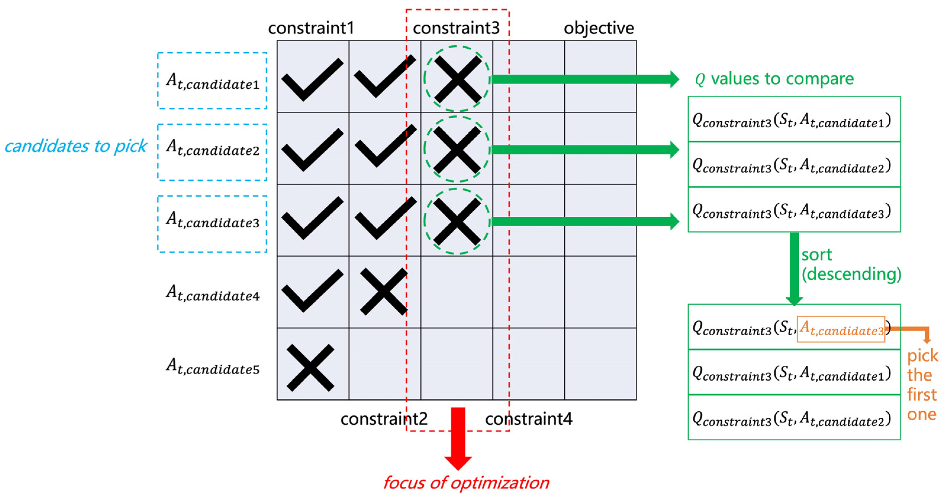
1. Test and filter action candidates, starting from the first constraint, until no candidates pass a specific test or all tests are passed. If all candidates fail on a constraint, the constraint becomes the focus of optimization; on the other hand, if there is at least one candidate satisfying all constraints (passing all the tests), the objective becomes the focus of optimization. Record the index of focus as $i$, $i\in \{constraint1,constraint2,\dots ,objective\}$.         2. Record indices of candidates reaching $i$ as $j_1,j_2,\dots$, $j_k\in \{candidates1,candidates2,\dots \}$.         3. Sort $Q_i\left(S_t,A_{j_1}\right),Q_i\left(S_t,A_{j_2}\right),\dots$ in descending order and pick the action corresponding to the first as $A_t$. If multiple actions attain the maximum $Q_i$ value at the same time, randomly pick one from them.

Take $A_t$, observe $R_{t+1},R_{t+1,constraint1},R_{t+1,constraint2},\dots$ and $S_{t+1}$

Append the vector         $move={\left[S_t,A_t,S_{t+1},R_{t+1},R_{t+1,constraint1},R_{t+1,constraint2},\dots \right]}^{\mathrm{T}}$     to $trajectory$: $trajectory\leftarrow \left[trajectory,move\right]$

Update the current state: $S_t\leftarrow S_{t+1}$

until the terminal state is reached

Update $Q_{objective},Q_{constraint1},Q_{constraint2},\dots$ with Monte Carlo,   according to the trajectory recoded

4. Simulation Results

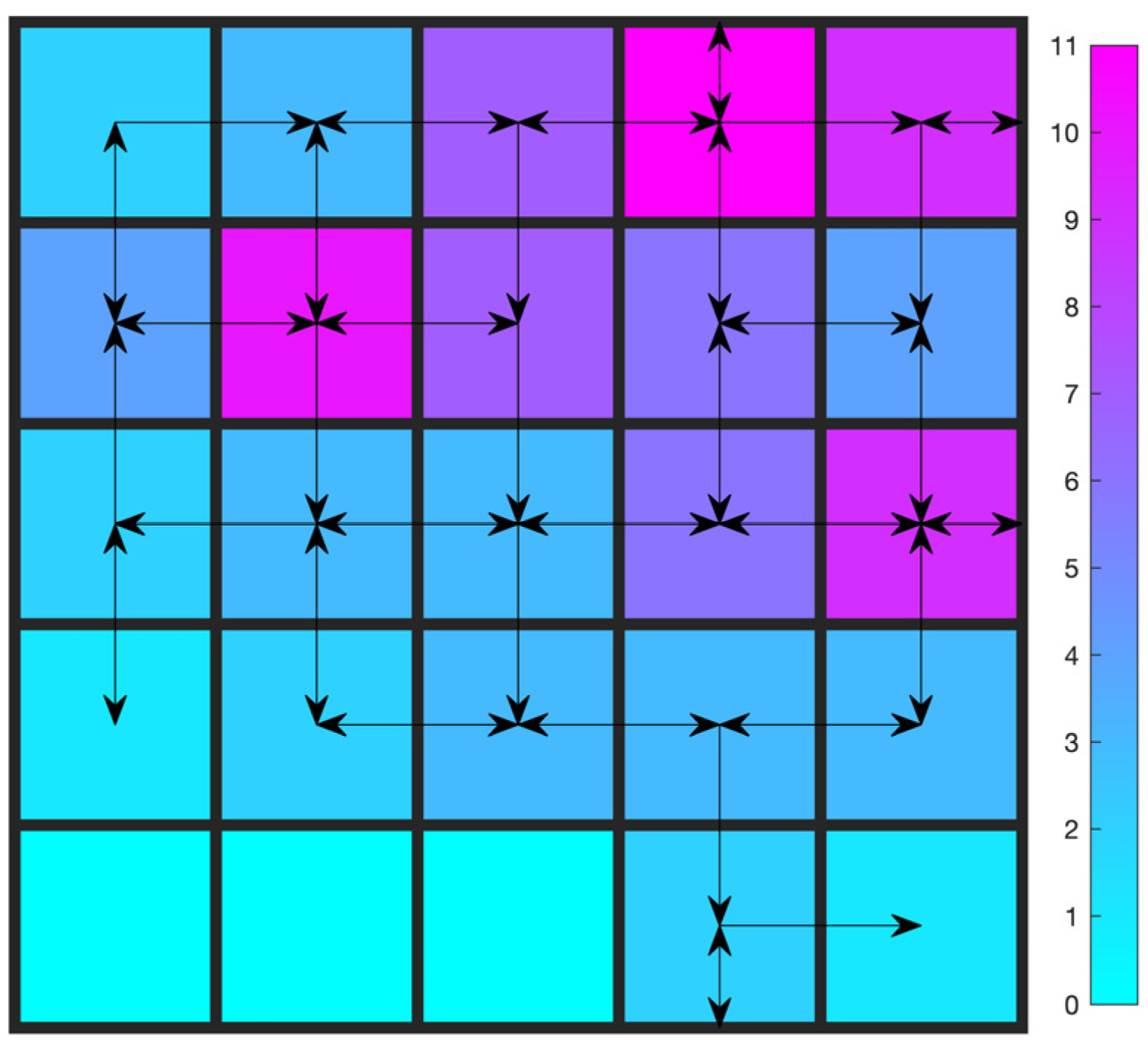
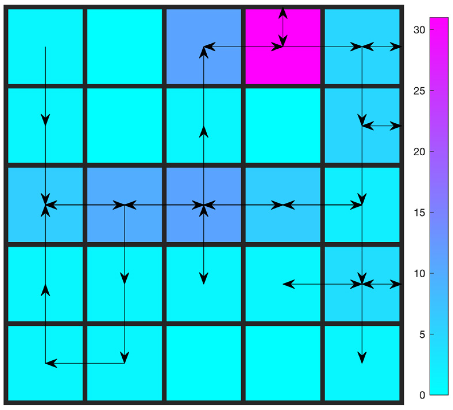
The effectiveness of the proposed Q-sorting is verified by two problems. The first one is the classic Gridworld, and the second one is the motor speed synchronization control. For both problems, cases of one constraint and two constraints are investigated. All learning processes start with random policies, which may be infeasible. The framework of Q-sorting can be applied to any value-based RL algorithm, like Monte Carlo or Q-learning. Here, for the simulation results, Monte Carlo is used. Source code and demos are provided in the supplementary materials.

4.1. Gridworld

A 5 × 5 Gridworld is considered, as shown in Figure 3. In the classic setting, the agent starts from the origin (the upper left) and tries to reach the destination (the lower right) with as few steps as possible. There are no constraints, but only the objective. In this paper, however, the Gridworld problem is adapted to include one or two constraints. In the case of one constraint, the agent collects three points upon each move (even those that leave the agent in the original position, like those against the wall). Throughout the whole episode, a minimum of 300 points is required. The objective is the same as that of the classic version: minimum steps. Upon simple inspection, it is quite easy to conclude that the optimal value of steps to reach the destination while satisfying the constraint is 100.

Simulation results are reported in Figure 4, which are obtained from 10 repeated simulations. The curve represents the mean, and the shaded region represents the standard deviation. The first two subplots show performances corresponding to the objective and the constraint, respectively. The last subplot illustrates the progress of the focus of optimization, as labeled in Figure 1. For a specific episode, the focus of optimization on each step is summed up and averaged over the whole episode to get the focus of episode, which is then plotted. All performance indices are averaged within a moving window containing the nearby 10 episodes.

From Figure 4, it can be observed that the averaged points collected are far above the constraint threshold at the very beginning of learning, which is the result of random policies upon initialization. On average, it takes the agent about 300 steps to reach the destination in the first episode, and the corresponding collected points are about 1000, which is certainly nonoptimal since the constraint requires only 300 points. After that, steps taken quickly approach the optimal value of 100, with the averaged points collected decreasing while staying above the constraint. With the decay of the exploration rate, the policy gradually converges to the optimal and feasible one, achieving the theoretically minimum number of steps 100.

The last subplot of Figure 4 shows the progress of the focus. Within the first 30 episodes, the focus value quickly climbs from 1, which corresponds to the constraint, to 2, which corresponds to the objective. This is because the random policies upon initialization easily satisfy the constraint. However, it is not always the case. A more difficult situation is presented later, where the agent has to consider another extra constraint.

The mechanism of filtering and sorting (Section 3) ensures that the agent considers the constraint in the first place while learning to maximize the return. This is reflected in the second subplot, where the points collected stay above the required threshold (300) most of the time. In other words, satisfaction with the constraint is ensured during the learning process, not just after the end of it.

The optimal trajectory after learning is shown in Figure 5. It is produced by executing the learned policy greedily. The color bar shows the number of visits for each cell.

The one-constraint Gridworld problem is then extended to include one more constraint: the number of turns. One turn is counted if both conditions are met: (a) the moving axis (either horizontal or vertical) of the current action is different from that of the previous one; (b) the current position is different from the previous one. At the beginning, the moving axis is undefined (null). The moving axis is updated only if the current position is different from the previous one.

In the simulation, two thresholds for the number of turns are tested. The first one is 20, the results of which are shown in Figure 6. The agent is required to collect at least 300 points with at most 20 turns, using as few steps as possible. It is to be noted that the constraint on the number of turns and the objective of the minimum steps are somehow contradictory. To constrain the number of turns, the agent is tempted to adopt a strategy that keeps going against the wall. However, doing so would probably increase the number of steps. It is difficult to balance the two. In the simulation, it was found that, apart from the horizontal and vertical positions, adding a third state variable, which represents the number of total steps taken so far, is helpful. And different from the first constraint, which is easily satisfied from the beginning by the random policies, the second constraint gets satisfied late in the middle of the learning. This is indicated by the third and last subplot of Figure 6, in which the focus index slowly increases from 1 to 3 and spends a lot of episodes around 2.

Trajectory after learning about the two-constraint Gridworld problem is shown in Figure 7. Comparing Figure 7 with Figure 5, the effects of the constraint on the number of turns are obvious. To satisfy the second constraint while collecting points, the agent adopts a strategy to keep going against the wall (the purple cell), which counts as no turns.

To make the comparison clearer, the threshold for the second constraint is further lowered from 20 to 5. Simulation results for the learning process and the trajectory after learning are shown in Figure 8 and Figure 9, respectively. It is a more difficult mission for the agent since now it has to collect at least 300 points with at most 5 turns. As a result, the focus index climbs more slowly than in Figure 4 and Figure 6. The agent spends a lot of time learning to constrain the number of turns to 5. After the end of learning, however, it successfully finds a policy that attains 300 points within 5 turns. In the final learned trajectory, the agent spends a lot of time on the lower left corner by going left against the wall.

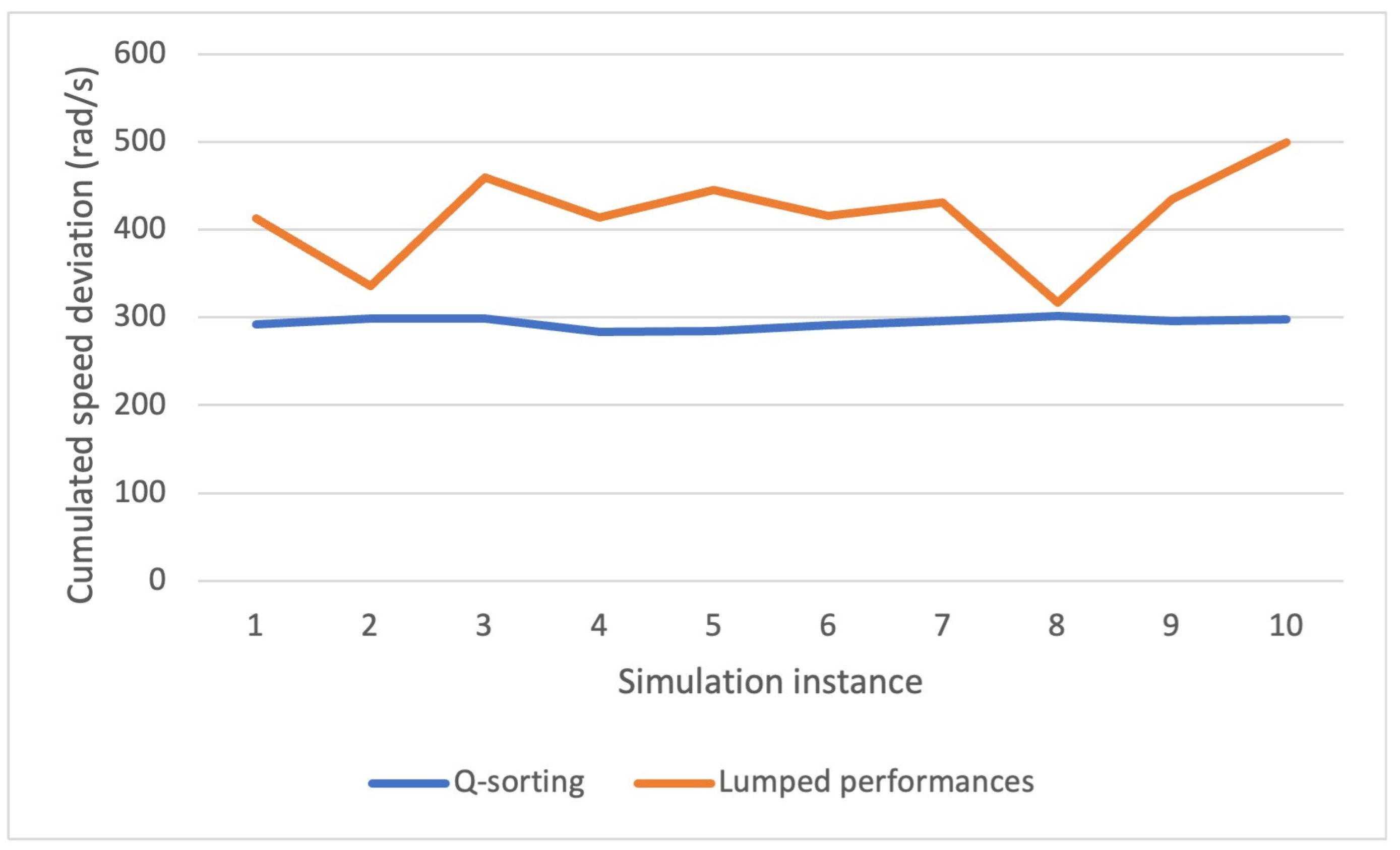
4.2. Motor Speed Synchronization Control

The motor speed synchronization problem can be found in [40,41]. To be short, the speed of the motor is required to change from an initial speed to a terminal one by following a reference trajectory. In this paper, it is modeled as a RL problem. The state variable is the time stamp, discretized with a step size of 0.1 s. The action variable is the motor torque, with the range $[-10,0]$ Nm for cases of one constraint and $[-10,5]$ Nm for cases of two constraints, both discretized with the quantization step $0.5$ Nm. A detailed problem setup can be found in the supplementary materials.

Two kinds of objectives are considered here. In the first one, the motor speed is required to decrease to negative values as fast as possible ($R_{t+1}=-1$). Whereas in the second one, it should be as slow as possible ($R_{t+1}=1$). As in the Gridworld problem, both cases of one constraint and two constraints are considered. In the case of one constraint, the sole requirement is that the deviation between the actual speed trajectory and the reference be smaller than a certain threshold. The deviation between two speed trajectories is calculated as ${\sum }_{t=0}{R}_{t+1,constraint1}$ where $R_{t+1,constraint1}$ is as follows:

$$R_{t+1,constraint1}=-\left|{\omega }_{t+1,ref}-{\omega }_{t+1,act}\right| (\mathrm{r}\mathrm{a}\mathrm{d}/\mathrm{s})$$

(5)

The reference speed trajectory is a simple line given by the following equation:

$${\omega }_{ref}\left(t\right)=\frac{{\omega }_0-{\omega }_T}{0-T}\cdot t+{\omega }_0$$

(6)

where ${\omega }_0=3000$ rpm (revolutions per minute), ${\omega }_T=0$, and $T=1$ s. In the case of two constraints, apart from the trajectory deviation, the number of “turns” by the actual motor speed along the whole process is also constrained to be larger than a certain value. Here, one “turn” is defined as a change in the sign of the rotational acceleration. For example, if the rotational acceleration of the motor is negative (the speed is going down) on the previous time step and positive (the speed is going up) on the current time step, it is counted as one turn. It will be interesting to see how the agent manages to satisfy both constraints.

Figure 10 shows motor speed trajectories after the end of learning for the two cases of objective under different thresholds of $c_1$ ranging from −600 to −100 rad/s. Cumulated $R_{t+1,constraint1}$ in Equation (2) against the threshold $c_1$ is also shown in the form ${\sum }_{t=0}{R}_{t+1,constraint1}$/$c_1$. If the value of ${\sum }_{t=0}{R}_{t+1,constraint1}$ is larger than that of $c_1$, the constraint is successfully satisfied.

It can be seen that all learned motor speed trajectories successfully satisfy the corresponding constraints. The objective performance index is also maximized, which can be inferred from the simulation results. For example, in the case where the objective is the shortest duration for the motor to reach negative speed values, if we tighten the constraint on deviation between the actual speed trajectory and the reference, the duration would be longer since the actual speed trajectory would have to lean towards the reference. On the other hand, if the constraint is loose, the duration would be shorter. The effects of the objective can also be observed by comparing the two subplots in Figure 10. For the shortest duration objective, speed trajectories are all under the reference, whereas for the longest duration objective, they are all above, which is reasonable.

Figure 11 shows simulation results for one of the instances in Figure 10, where the objective is the longest duration and the constraint threshold $c_1$ is −100 rad/s. This requires that the cumulated speed deviation along the whole process does not exceed 100 rad/s, which is quite a difficult task. As a result, the focus index increases at a rather slow pace because the agent spends a lot of time learning to satisfy the constraint. It is near the end of learning that the agent starts to consider the objective completely. The return settles on the optimal value 11, which corresponds to a duration of 1.1 s (because the time step is 0.1 s and the agent gets one unit reward upon each transition along the timeline), after about 2000 episodes. The constraint is satisfied after about 1500 episodes.

To further emphasize the effectiveness of the algorithm in satisfying the constraint while pursuing optimality, performances regarding different levels of the constraint in the process of learning are shown in Figure 12. The objective is the longest duration for the motor to reach negative speed values. Three levels of the constraint are compared, namely, $c_1=-1000$ rad/s, $c_1=-600$ rad/s, and $c_1=-\infty$ (which corresponds to the case of no constraints). It can be inferred that if no constraints are posed, the optimal policy is to output the maximum torque possible on each time step, which will also result in the maximum deviation from the reference speed trajectory. This is exactly the case in Figure 12, when $c_1=-\infty$. However, if specific constraints are posed for the level of deviation, the objective performance will be compromised in order to satisfy the constraint. Notice how the agent pushes itself against the limit of the constraint to maintain satisfaction with it while pursuing optimal objective performance. The tighter the constraint, the smaller the return.

Simulation results for the case of two constraints are shown in Figure 13, where $c_1$ for the first constraint is fixed to −500 rad/s. As has been discussed before, the second constraint corresponds to the number of “turns”, that is, the speed going up and down. A comparison between Figure 10 and Figure 13 will reveal the effects of the second constraint. If the number of speed turns is unconstrained, under the threshold $c_1=-500$ rad/s, the shortest duration for the motor to reach negative speed values is 0.6 s, according to Figure 10. However, if at least three or four turns are required, the shortest duration will increase to 0.8 s, according to Figure 13. This seems natural since alternating between acceleration and deceleration takes the agent more time to reach the target speed than full deceleration. In the second subplot of Figure 13, the first constraint is slightly violated (−500.828 vs. −500), which may be due to the inaccuracy of the learned function values. Figure 14 shows simulation results for one of the instances in Figure 13a, where the objective is the shortest duration with cumulative constraints $c_1=-500$ rad/s and $c_2=4$ turns. The agent learns to satisfy the first constraint after about 10 episodes and the second one after about 150 episodes.

Last but not least, the results of Q-sorting are compared with the method of lumped performances (LP), which integrates constraints into the objective function and turns the original problem into a constraint-free one. LP is, in effect, the Lagrangian relaxation with a fixed multiplier. Here, only one constraint is considered, namely, the deviation from the reference. Specifically, the reward signal is modified as follows:

$$R_{t+1,lumped}=\left\{\begin{array}{cc}-1-\beta \left|{\omega }_{t+1,ref}-{\omega }_{t+1,act}\right|,& \mathrm{o}\mathrm{b}\mathrm{j}\mathrm{e}\mathrm{c}\mathrm{t}\mathrm{i}\mathrm{v}\mathrm{e}:\mathrm{s}\mathrm{h}\mathrm{o}\mathrm{r}\mathrm{t}\mathrm{e}\mathrm{s}\mathrm{t}\mathrm{d}\mathrm{u}\mathrm{r}\mathrm{a}\mathrm{t}\mathrm{i}\mathrm{o}\mathrm{n}\\ 1-\beta \left|{\omega }_{t+1,ref}-{\omega }_{t+1,act}\right|,& \mathrm{o}\mathrm{b}\mathrm{j}\mathrm{e}\mathrm{c}\mathrm{t}\mathrm{i}\mathrm{v}\mathrm{e}:\mathrm{l}\mathrm{o}\mathrm{n}\mathrm{g}\mathrm{e}\mathrm{s}\mathrm{t}\mathrm{d}\mathrm{u}\mathrm{r}\mathrm{a}\mathrm{t}\mathrm{i}\mathrm{o}\mathrm{n}\end{array}\right.$$

(7)

The effects of the original constraint are controlled by the parameter $\beta$. Figure 15 shows learned speed trajectories for different values of $\beta$, ranging from 0.001, 0.003, …, to 0.025. For each trajectory, the deviation from the reference, the return, and the value of $\beta$ are shown, respectively. Obviously, the smaller the $\beta$, the smaller the effects of the constraint, and the larger the deviation from the reference. Figure 15 coincides with intuition. It is also observed that speed trajectories resulting from different values of $\beta$ exhibit similar shapes to those in Figure 10.

The method of LP comes with two main drawbacks. First, the relationship between the effects of the constraints and the value of $\beta$ is unclear. For example, one cannot easily determine the value of $\beta$ to express the requirement that the cumulated speed deviation should be below 300 rad/s. To attain a proper value of $\beta$, lots of trials and experiments are needed. Comparatively, in Q-sorting, the constraint is fed directly into the algorithm; no other proxy parameters are needed.

The second drawback is related to the performance consistency of the algorithm. Figure 16 shows motor speed trajectories for Q-sorting and LP, simulations of which are run repeatedly for 10 times each. The objective for both is to decrease the motor speed to negative values with as long a duration as possible. For Q-sorting, the cumulated speed deviation from the reference is required to be within 300 rad/s. For LP, it is controlled through the proxy parameter $\beta$, whose value is fixed to 0.005. Here, the value of $\beta$ is determined from Figure 15b, where the cumulated speed deviation (the constraint) is 275.2579 rad/s when $\beta =0.005$. The idea is to choose a value that results in a cumulated speed deviation near 300 rad/s.

Figure 17 shows the cumulated speed deviation for both methods in different simulation instances. Q-sorting provides great consistency, with the cumulative performance index concentrating around 300 rad/s, most of the time below it, just as the constraint requires. Comparatively, it ranges from 300 to 500 rad/s in the cases of LP, which implies that there is no deterministic relationship between the values of $\beta$ and the cumulative performance index of the constraint. One cannot count on the fixed value of $\beta$ for the satisfaction of a certain cumulative constraint. For reference, the standard deviations of the cumulated speed deviation for Q-sorting and LP over 10 repeated simulation runs are 6.1920 and 54.2635 rad/s, respectively.

In a word, compared to the conventional LP, Q-sorting not only provides greater ease of use by requiring only the constraint thresholds rather than trials and errors on the values of proxy parameters but also ensures better performance consistency and is thus more suitable for practical use.

5. Conclusions

An algorithm named Q-sorting for RL problems with multiple cumulative constraints is proposed. The core is a mechanism that dynamically determines the focus of optimization among different constraints/objective, at each step of learning. The focus and the action are determined through filtering and sorting of the Q table, which gives it the name Q-sorting. It is a plugin that can be readily applied to any value-based RL algorithm to provide the capability of satisfying cumulative constraints while pursuing optimality. It is verified with two adapted problems, namely, Gridworld and the motor speed synchronization control, each with one or two cumulative constraints. Simulation results show that the proposed method is able to learn an optimal policy that honors all cumulative constraints both during and after the learning process. This makes it suitable for safety-critical applications.

It has to be emphasized that although the idea of Q-sorting is effective, its performance heavily depends on the accuracy of Q values. That is because the algorithm uses $Q_{constraint}(S_t,a)$ to predict whether a specific action violates the constraint. An implementation developed in MATLAB using Monte Carlo to learn the value function is provided in the supplementary materials. Other tabular methods, such as Q-learning and SARSA, are also possible, but performances may differ.

This paper restricts the scenario to finite-time, episodic problems with deterministic environments and policies. Under this assumption, a determined policy with the same initial state will always result in the same cumulative performance index, so there is no need to express the cumulative constraints as expected/averaged values over multiple episodes. In problems with stochastic environments and policies, however, cumulative constraints can only be represented in an expected/averaged manner. Also, for problems with a discounted rather than episodic setting, it is sometimes desired to limit the average resources consumed on each step rather than the cumulated quantities. How to extend the idea of Q-sorting to the two cases above can be a future topic.

References

1. Sutton, R.S.; Barto, A.G. Reinforcement Learning: An Introduction; MIT Press: Cambridge, MA, USA, 2018; ISBN 978-0-262-19398-6. [Google Scholar]
2. Mnih, V.; Kavukcuoglu, K.; Silver, D.; Graves, A.; Antonoglou, I.; Wierstra, D.; Riedmiller, M. Playing Atari with Deep Reinforcement Learning. Nature 2013, 518, 529–533. [Google Scholar] [CrossRef] [PubMed]
3. Silver, D.; Huang, A.; Maddison, C.J.; Guez, A.; Sifre, L.; Van Den Driessche, G.; Schrittwieser, J.; Antonoglou, I.; Panneershelvam, V.; Lanctot, M.; et al. Mastering the Game of Go with Deep Neural Networks and Tree Search. Nature 2016, 529, 484. [Google Scholar] [CrossRef] [PubMed]
4. Geibel, P. Reinforcement Learning for MDPs with Constraints; Lecture Notes in Computer Science (including Subseries Lecture Notes in Artificial Intelligence Lecture Notes Bioinformatics); Springer: Berlin/Heidelberg, Germany, 2006; Volume 4212, pp. 646–653. [Google Scholar] [CrossRef]
5. Julian, D.; Chiang, M.; O’Neill, D.; Boyd, S. QoS and Fairness Constrained Convex Optimization of Resource Allocation for Wireless Cellular and Ad Hoc Networks. In Proceedings of the Twenty-First Annual Joint Conference of the IEEE Computer and Communications Societies, New York, NY, USA, 23–27 June 2002; IEEE: Piscataway, NJ, USA, 2002; Volume 2, pp. 477–486. [Google Scholar]
6. Yuan, J.; Yang, L. Predictive Energy Management Strategy for Connected 48V Hybrid Electric Vehicles. Energy 2019, 187, 115952. [Google Scholar] [CrossRef]
7. Zhang, R.; Xiong, K.; Lu, Y.; Fan, P.; Ng, D.W.K.; Letaief, K.B. Energy Efficiency Maximization in RIS-Assisted SWIPT Networks with RSMA: A PPO-Based Approach. IEEE J. Sel. Areas Commun. 2023, 41, 1413–1430. [Google Scholar] [CrossRef]
8. Zhang, R.; Xiong, K.; Lu, Y.; Gao, B.; Fan, P.; Letaief, K. Ben Joint Coordinated Beamforming and Power Splitting Ratio Optimization in MU-MISO SWIPT-Enabled HetNets: A Multi-Agent DDQN-Based Approach. IEEE J. Sel. Areas Commun. 2022, 40, 677–693. [Google Scholar] [CrossRef]
9. Liu, Y.; Halev, A.; Liu, X. Policy Learning with Constraints in Model-Free Reinforcement Learning: A Survey. In Proceedings of the IJCAI International Joint Conference on Artificial Intelligence, Montreal, QC, Canada, 19–27 August 2021; pp. 4508–4515. [Google Scholar] [CrossRef]
10. Altman, E. Constrained Markov Decision Processes; Routledge: Oxfordshire, UK, 1999; ISBN 1315140225. [Google Scholar]
11. Chow, Y.; Ghavamzadeh, M.; Janson, L.; Pavone, M. Risk-Constrained Reinforcement Learning with Percentile Risk Criteria. J. Mach. Learn. Res. 2018, 18, 6070–6120. [Google Scholar]
12. Tessler, C.; Mankowitz, D.J.; Mannor, S. Reward Constrained Policy Optimization. In Proceedings of the 7th International Conference on Learning Representations, ICLR 2019, New Orleans, LA, USA, 6–9 May 2019; pp. 1–15. [Google Scholar]
13. Bohez, S.; Abdolmaleki, A.; Neunert, M.; Buchli, J.; Heess, N.; Hadsell, R. Value Constrained Model-Free Continuous Control. arXiv 2019, arXiv:1902.04623. [Google Scholar]
14. Jayant, A.K.; Bhatnagar, S. Model-Based Safe Deep Reinforcement Learning via a Constrained Proximal Policy Optimization Algorithm. Adv. Neural Inf. Process. Syst. 2022, 35, 24432–24445. [Google Scholar]
15. Panageas, I.; Piliouras, G.; Wang, X. First-Order Methods Almost Always Avoid Saddle Points: The Case of Vanishing Step-Sizes. Adv. Neural Inf. Process. Syst. 2019, 32, 6474–6483. [Google Scholar]
16. Vidyasagar, M. Nonlinear Systems Analysis; SIAM: Philadelphia, PA, USA, 2002; ISBN 0898715261. [Google Scholar]
17. Glynn, P.W.; Zeevi, A. Bounding Stationary Expectations of Markov Processes; Institute of Mathematical Statistics: Waite Hill, OH, USA, 2008; Volume 4, pp. 195–214. [Google Scholar] [CrossRef]
18. Chow, Y.; Nachum, O.; Duenez-Guzman, E.; Ghavamzadeh, M. A Lyapunov-Based Approach to Safe Reinforcement Learning. Adv. Neural Inf. Process. Syst. 2018, 31, 8092–8101. [Google Scholar]
19. Chow, Y.; Nachum, O.; Faust, A.; Duenez-Guzman, E.; Ghavamzadeh, M. Lyapunov-Based Safe Policy Optimization for Continuous Control. arXiv 2019, arXiv:1901.10031. [Google Scholar]
20. Satija, H.; Amortila, P.; Pineau, J. Constrained Markov Decision Processes via Backward Value Functions. In Proceedings of the 37th International Conference on Machine Learning, ICML 2020, Virtual, 13–18 July 2020; pp. 8460–8469. [Google Scholar]
21. Achiam, J.; Held, D.; Tamar, A.; Abbeel, P. Constrained Policy Optimization. In Proceedings of the International Conference on Machine Learning; PMLR, Sydney, Australia, 6–11 August 2017; pp. 22–31. [Google Scholar]
22. Schulman, J.; Levine, S.; Abbeel, P.; Jordan, M.; Moritz, P. Trust Region Policy Optimization. In Proceedings of the International Conference on Machine Learning, PMLR, Lille, France, 7–9 July 2015; Volume 67, pp. 1889–1897. [Google Scholar]
23. Liu, Y.; Ding, J.; Liu, X. IPO: Interior-Point Policy Optimization under Constraints. In Proceedings of the AAAI 2020-34th AAAI Conference on Artificial Intelligence, New York, NY, USA, 7–12 February 2020; pp. 4940–4947. [Google Scholar] [CrossRef]
24. Boyd, S.P.; Vandenberghe, L. Convex Optimization; Cambridge University Press: Cambridge, UK, 2004; ISBN 0521833787. [Google Scholar]
25. Liu, Y.; Ding, J.; Liu, X. A Constrained Reinforcement Learning Based Approach for Network Slicing. In Proceedings of the 2020 IEEE 28th International Conference on Network Protocols (ICNP), Madrid, Spain, 13–16 October 2020. [Google Scholar] [CrossRef]
26. Liu, Y.; Ding, J.; Liu, X. Resource Allocation Method for Network Slicing Using Constrained Reinforcement Learning. In Proceedings of the 2021 IFIP Networking Conference (IFIP Networking), Espoo and Helsinki, Finland, 21–24 June 2021; pp. 1–3. [Google Scholar] [CrossRef]
27. Wei, H.; Liu, X.; Ying, L. Triple-Q: A Model-Free Algorithm for Constrained Reinforcement Learning with Sublinear Regret and Zero Constraint Violation. Proc. Mach. Learn. Res. 2022, 151, 3274–3307. [Google Scholar]
28. Rummery, G.; Niranjan, M. On-Line Q-Learning Using Connectionist Systems (Technical Report); University of Cambridge, Department of Engineering Cambridge: Cambridge, UK, 1994; Volume 37. [Google Scholar]
29. Wei, C.Y.; Jafarnia-Jahromi, M.; Luo, H.; Sharma, H.; Jain, R. Model-Free Reinforcement Learning in Infinite-Horizon Average-Reward Markov Decision Processes. In Proceedings of the 37th International Conference on Machine Learning ICML 2020, Virtual, 13–18 July 2020; pp. 10101–10111. [Google Scholar]
30. Singh, R.; Gupta, A.; Shroff, N.B. Learning in Constrained Markov Decision Processes. IEEE Trans. Control Netw. Syst. 2023, 10, 441–453. [Google Scholar] [CrossRef]
31. Bura, A.; HasanzadeZonuzy, A.; Kalathil, D.; Shakkottai, S.; Chamberland, J.F. DOPE: Doubly Optimistic and Pessimistic Exploration for Safe Reinforcement Learning. Adv. Neural Inf. Process. Syst. 2022, 35, 1047–1059. [Google Scholar]
32. Yang, T.Y.; Rosca, J.; Narasimhan, K.; Ramadge, P.J. Projection-Based Constrained Policy Optimization. In Proceedings of the 8th International Conference on Learning Representations, ICLR 2020, Addis Ababa, Ethiopia, 26–30 April 2020; pp. 1–24. [Google Scholar]
33. Morimura, T.; Peters, J. Derivatives of Logarithmic Stationary Distributions for Policy Gradient Reinforcement Learning. Neural Comput. 2010, 22, 342–376. [Google Scholar] [CrossRef] [PubMed]
34. Pankayaraj, P.; Varakantham, P. Constrained Reinforcement Learning in Hard Exploration Problems. In Proceedings of the 37th AAAI Conference on Artificial Intelligence, AAAI 2023, Washington, DC, USA, 7–14 February 2023; Volume 37, pp. 15055–15063. [Google Scholar] [CrossRef]
35. Calvo-Fullana, M.; Paternain, S.; Chamon, L.F.O.; Ribeiro, A. State Augmented Constrained Reinforcement Learning: Overcoming the Limitations of Learning with Rewards. IEEE Trans. Automat. Control, 2023; early access. [Google Scholar] [CrossRef]
36. McMahan, J.; Zhu, X. Anytime-Constrained Reinforcement Learning. Proc. Mach. Learn. Res. 2024, 238, 4321–4329. [Google Scholar]
37. Bai, Q.; Bedi, A.S.; Agarwal, M.; Koppel, A.; Aggarwal, V. Achieving Zero Constraint Violation for Constrained Reinforcement Learning via Primal-Dual Approach. In Proceedings of the 36th AAAI Conference on Artificial Intelligence, AAAI 2022, Virtually, 22 February–1 March 2022; Volume 36, pp. 3682–3689. [Google Scholar] [CrossRef]
38. Ma, Y.J.; Shen, A.; Bastani, O.; Jayaraman, D. Conservative and Adaptive Penalty for Model-Based Safe Reinforcement Learning. In Proceedings of the 36th AAAI Conference on Artificial Intelligence, AAAI 2022, Virtually, 22 February–1 March 2022; Volume 36, pp. 5404–5412. [Google Scholar] [CrossRef]
39. Xu, H.; Zhan, X.; Zhu, X. Constraints Penalized Q-Learning for Safe Offline Reinforcement Learning. In Proceedings of the 36th AAAI Conference on Artificial Intelligence, AAAI 2022, Virtually, 22 February–1 March 2022; Volume 36, pp. 8753–8760. [Google Scholar] [CrossRef]
40. Huang, J.; Zhang, J.; Huang, W.; Yin, C. Optimal Speed Synchronization Control with Disturbance Compensation for an Integrated Motor-Transmission Powertrain System. J. Dyn. Syst. Meas. Control 2018, 141, 041001. [Google Scholar] [CrossRef]
41. Huang, J.; Zhang, J.; Yin, C. Comparative Study of Motor Speed Synchronization Control for an Integrated Motor–Transmission Powertrain System. Proc. Inst. Mech. Eng. Part D J. Automob. Eng. 2020, 234, 1137–1152. [Google Scholar] [CrossRef]
Figure 1. Q-sorting.
Mathematics 12 02001 g001
Figure 2. Optimization of the policy.
Mathematics 12 02001 g002
Figure 3. Gridworld.
Mathematics 12 02001 g003
Figure 4. Simulation results: Gridworld with one constraint.
Mathematics 12 02001 g004
Figure 5. Trajectory after learning: Gridworld with one constraint.
Mathematics 12 02001 g005
Figure 6. Simulation results: Gridworld with two constraints (20 turns at most).
Mathematics 12 02001 g006
Figure 7. Trajectory after learning: Gridworld with two constraints (20 turns at most).
Mathematics 12 02001 g007
Figure 8. Simulation results: Gridworld with two constraints (5 turns at most).
Mathematics 12 02001 g008
Figure 9. Trajectory after learning: Gridworld with two constraints (5 turns at most).
Mathematics 12 02001 g009
Figure 10. Motor speed trajectory after learning (one constraint), x/y is for t = 0 R t + 1 , c o n s t r a i n t 1 / c 1 . (a) Objective: shortest duration and (b) objective: longest duration.
Mathematics 12 02001 g010
Figure 11. Simulation results: motor speed synchronization control with one constraint (objective: longest duration; constraint: c 1 = 100 rad/s).
Mathematics 12 02001 g011
Figure 12. Simulation results: motor speed synchronization control with different levels of the constraint (objective: longest duration).
Mathematics 12 02001 g012
Figure 13. Motor speed trajectories after learning (two constraints), x1|x2/y1|y2 is for t = 0 R t + 1 , c o n s t r a i n t 1 | t = 0 R t + 1 , c o n s t r a i n t 2 / c 1 | c 2 . (a) Objective: shortest duration and (b) objective: longest duration.
Mathematics 12 02001 g013
Figure 14. Simulation results: motor speed synchronization control with two constraints (objective: shortest duration; constraints: c 1 = 500 rad/s and c 2 = 4 turns).
Mathematics 12 02001 g014
Figure 15. Motor speed trajectories after learning for LP (one constraint). (a) Objective: shortest duration and (b) objective: longest duration.
Mathematics 12 02001 g015
Figure 16. Motor speed trajectories for Q-sorting and LP over 10 runs (objective: longest duration). (a) Q-sorting and (b) LP.
Mathematics 12 02001 g016
Figure 17. Cumulated speed deviation over 10 runs.
Mathematics 12 02001 g017
Disclaimer/Publisher’s Note: The statements, opinions and data contained in all publications are solely those of the individual author(s) and contributor(s) and not of MDPI and/or the editor(s). MDPI and/or the editor(s) disclaim responsibility for any injury to people or property resulting from any ideas, methods, instructions or products referred to in the content.