A Rate of Change and Center of Gravity Approach to Calculating Composite Indicator Thresholds: Moving from an Empirical to a Theoretical Perspective


Abstract
:1. Introduction
2. Literature Review
2.1. Common Threshold Setting Approaches
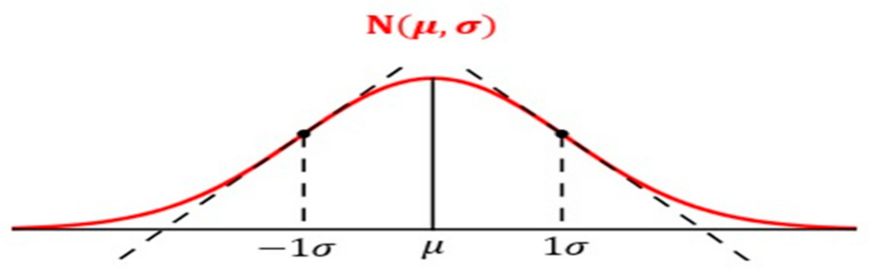
- Empirical–Statistical Approach
- The Z equation is defined as Z = (X − μ)/σ,
- Z = transformed value (measured in standard deviation units);
- X = value to be transformed (from the original dataset);
- μ = arithmetic average of the distribution;
- σ = standard deviation of the distribution.
- Trisect Method
- Max–Min Method
- Union of Minima
2.2. Proposed Principles for Composite Indicators Thresholds
- a.
- Thresholds must be independent of the data and/or alternatives to be evaluated.
- b.
- Thresholds must take into consideration the equivalence value of the elements that make up the measurement scale (its transformation function) to determine their rate of change at the equilibrium point and, from there, determine the best value for the scale threshold.
2.3. An RCCG Approach to Local Threshold Calculation: A Geometric Explanation
3. Theoretical Framework
3.1. Brief Mathematical Discussion of AHP/ANP Absolute Models and Their Use for Composite Indicators
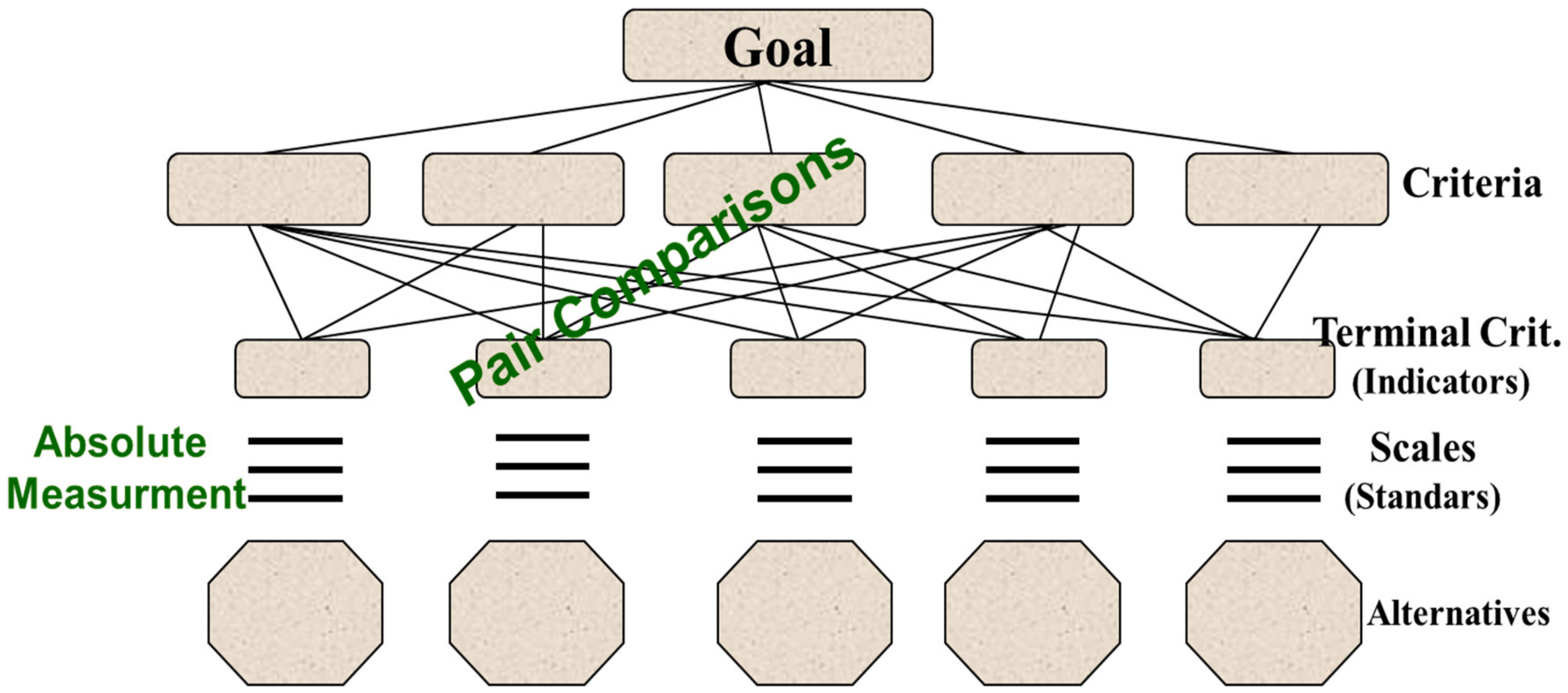
3.1.1. AHP Hierarchical Superposition Principle
- i = number of levels of the hierarchy;
- j = number of terminal criteria of the hierarchy (the measurement indicators);
- k = alternative number;
- wij = weight of criterion j at the level I;
- Sj(Alk) = local evaluation of alternative k in the scale belonging to the terminal criteria j (the measurement indicator j); the evaluation is made with a rating scale (the transformation function) in the absolute measurement mode;
- Agk = global evaluation of alternative k, evaluated in all terminal criteria (the measurement indicators).
3.1.2. Eigenvector Operator (Calculating the Weights)
- e = unitary vector {1,…,1};
- (A) = pairwise comparison matrix;
- W(i) = eigenvector, i.e., an absolute metric scale for complex systems;
- CI = consistency index (one wants to be as close as possible to the “n” value);
- RI = random consistency index (one wants to be as far away as possible to this value);
- CR = consistency ratio (CR ≤ 10% is considered an acceptable consistency ratio);
- N = dimension of the PCM.
3.2. AHP/ANP Relative and Absolute Measurement
3.3. Scales, Invariants and Thresholds
3.3.1. Scales
- Types of most used scales
- Nominal Scale: Invariant under one-to-one correspondence (bijective function).
- Ordinal Scale: Invariant against monotonic transformations.
- Interval Scale: Invariant against the transformation Y = a * X + b, with positive a and b.
- Ratio Scale: Invariant against the transformation Y = a * X, with “a” positive.
- Absolute Ratio Scale: Invariant against the transformation Y = X (identity function).
3.3.2. Examples of Thresholds in Scale Types
3.3.3. Representativeness of the Measurement Scale
3.4. PCM as a Transformation Function
3.5. Conclusions about Scales
- The complexity of the problem to be solved normally leads to the use of a large number of variables and indicators, aimed at analyzing the available alternatives.
- These indicators and scales must be specific to the problem and independent of their qualitative or quantitative nature.
- The AHP/ANP provides a mechanism with which to construct measurement and cardinal scales for all types of intensity scales. Only scales that constitute a measure have the arithmetic properties necessary to synthetize the many scales present in an AHP/ANP model, combine results from and to other methods, and perform sensitivity and stability analyses.
- The coordinates of a PCM eigenvector can be visualized as a transformation function, from ordinal to cardinal, in a coordinate plane.
- It is important to understand the nature and properties of the scales used by each methodology to use them appropriately (this is the responsibility of the professional user).
- Technological development has created an extensive number of figures and data. The challenge is to determine the relevant variables of a problem and find the necessary data and its representativeness or importance to evaluate the alternatives within the context of the problem.
- Numbers are important, but knowledge is even more important. Numbers, by themselves, may be totally invalid, useless, or irrelevant.
4. Calculation of the Local Threshold of a Scale
- Transformation function (vector of priorities of the scale at the equilibrium point);
- Rate of change (at the equilibrium point);
- Center of gravity (at the equilibrium point).
4.1. Transformation Function
| Indicator: Insufficient Level of Education | |||||
| Level | High | Moderate | Low | Very Low | Null |
| Value | 1 | 0.5524 | 0.1736 | 0.0847 | 0 |
4.2. Rate of Change
4.3. Center of Gravity
4.4. Application of an RCCG Approach in a Risk Model
4.5. Construction of LT Calculation Function
- It considers balance in terms of the parameters of the function; that is, if one parameter is changed, the other will also change to compensate (concept of center of gravity).
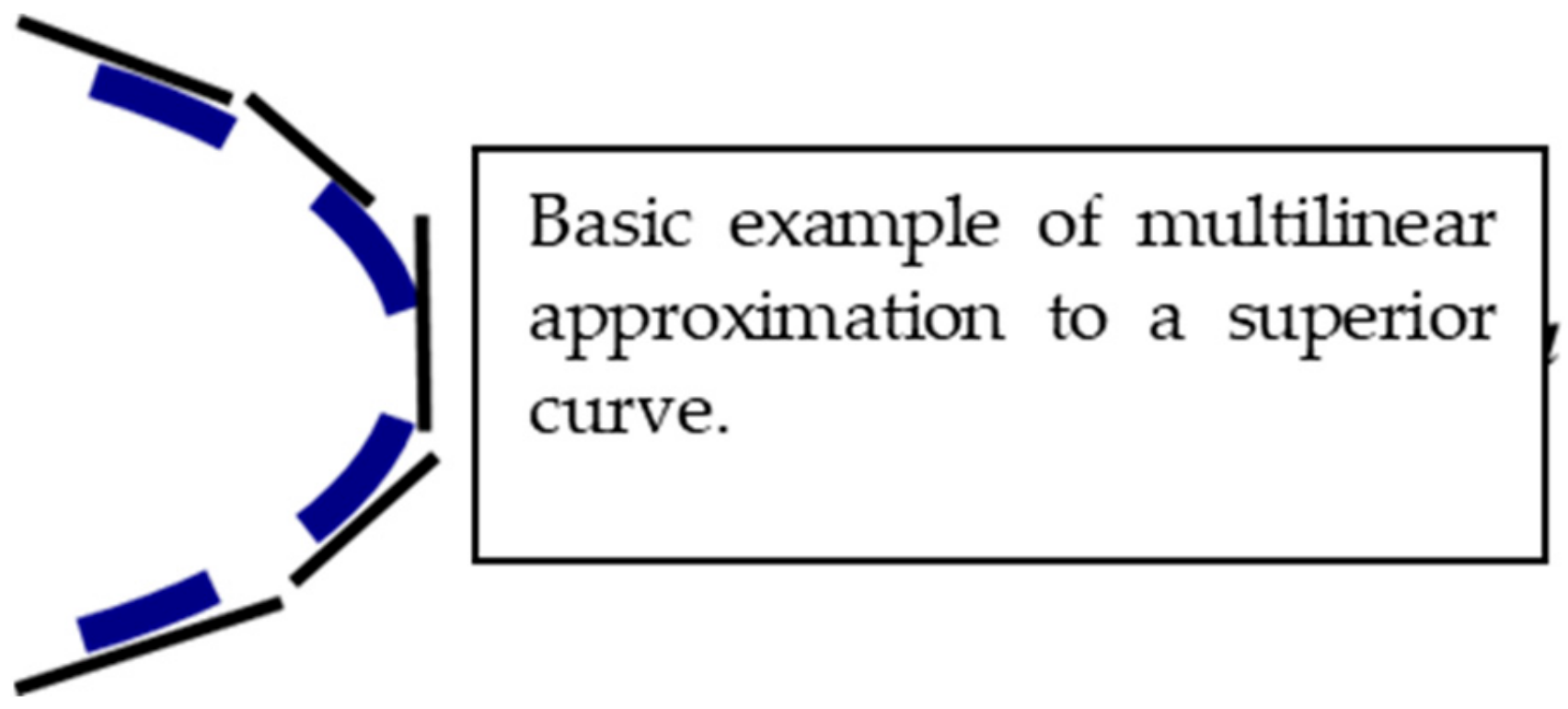
- It is always possible to interpolate a nonlinear function constructed by points using a weighted linear function as long as it is between two adjacent points of the function to be approximated (Taylor application).
4.6. Rate of Change and Center of Gravity in a Benefits Model
- 1.
- It is supposed that LT is located between the adjacent levels M and L. Although this is the general case, sometimes, the adjacent levels may be others. For example, LT could lie between the levels M = moderate and H = high, which would be strange in a risk model but not impossible. In this case, it is enough to replace “M” with “H” and “L” with “M” in Equation (9).
- 2.
- In a risks model, the aim is to stress the risk (maximum tolerable risk); while in a benefits model, the aim is to stress the benefit (minimum acceptable or tolerable benefit).
- 3.
- In a benefits model, the treatment is the same, but the reference point is changed to the highest level and the direction of the arrow is going down (reversed with respect to Figure 10). In this example, we take the reference point (RP) on M and go down through the transformation function. This is because in a profit model, one must start from the highest level and look for the minimum tolerable profit (profit threshold of the scale).
4.7. Some Singular and Reference Points for Risks and Benefits Models
- The Average point:
- Binary Scales:
- Special situations:
- Extreme Values in a Risk Model:
- Extreme Values in a Benefits Model:
4.8. Example of LT Calculation for a Risk Model
4.8.1. Interpretation of this Procedure by the Expert
4.8.2. Conclusion for the Local Threshold LT
4.8.3. Compensatory and Non-Compensatory Method
4.9. Global Threshold (GT)
- GT = global threshold;
- LTi = local threshold of indicator “i”;
- WGi = global weight of indicator “i”.
4.10. Combining Global Threshold with Compatibility Index G
4.10.1. Conditions of use
- Belonging and Representation
- Consistency
- Normalization
4.10.2. Properties
- Non-Negativity
- Triangular Inequality
4.10.3. Threshold of Compatibility
4.11. Calculation of Combining GT with G
- To avoid unwanted compensation;
- To avoid discarding a consensual alternative (acceptable for the majority) that does not comply with the GT condition in advance.
- I = indicator that makes the maximum contribution to G if the alternative changes its value in the scale;
- w(i) = weight of indicator “i”;
- G (Ai; TPi) = compatibility between the profiles of the alternative and the threshold profile in the “i” indicator.
4.12. Combining Two or More Models
4.13. Some Final Thoughts about Scales and Thresholds
- Scales of measurement
- Local and global thresholds
- 1.
- The local thresholds, and especially the global threshold, must represent an external element with respect to the set of alternatives and not be affected by the values that they may have; otherwise, adding, changing, or eliminating alternatives will cause the threshold values to vary, and this (in general) is not reasonable. The phrase “in general” is in parentheses because there are very particular cases where this could, in fact, be reasonable.
- 2.
- The global threshold must depend on the importance (the weight) of the terminal criteria (the indicators). In this way, the global threshold value will reflect the relative importance of the model components in the same way as the alternatives do, ensuring that it is applying the same rule of measurement in both cases. Furthermore, this form of building the global threshold makes it possible to build a virtual alternative (the threshold profile or TP) and to compare the specific behaviors of every alternative through the compatibility index G and not just their final value (the global threshold), which is not always a sufficient condition, as explained in Section 4.11.
5. Final Conclusions
Author Contributions
Funding
Data Availability Statement
Conflicts of Interest
Appendix A

| Item | Author(s) | Year | Title | Publication | Volume | Issue |
|---|---|---|---|---|---|---|
| 1 | Szabo, Zsuzsanna Katalin; Szadoczki, Zsombor; Bozoki, Sandor; Stanciulescu, Gabriela C.; Szabo, Dalma | 2021 | An Analytic Hierarchy Process Approach for Prioritisation of Strategic Objectives of Sustainable Development | Sustainability | 13 | 4 |
| 2 | Mao, Feng; Zhao, Xianfu; Ma, Peiming; Chi, Shiyun; Richards, Keith; Clark, Julian; Hannah, David M.; Krause, Stefan | 2019 | Developing composite indicators for ecological water quality assessment based on network interactions and expert judgment | Environmental Modelling & Software | 115 | |
| 3 | Ma Zhaipu; Zhao Jianhua; Wu Ling; Shi Changcan; Zhang Chunquan | 2010 | The quantitative research of composite immune indicator for crustacean | Fish & Shellfish Immunology | 28 | 1 |
| 4 | Wong, Antony King Fung; Kim, Seongseop (Sam); Lee, Suna; Elliot, Statia | 2021 | An application of Delphi method and analytic hierarchy process in understanding hotel corporate social responsibility performance scale | Journal of Sustainable Tourism | 29 | 7 |
| 5 | Orencio, Pedcris M.; Fujii, Masahiko | 2013 | A localized disaster-resilience index to assess coastal communities based on an analytic hierarchy process (AHP) | International Journal of Disaster Risk Reduction | 3 | |
| 6 | Zebardast, Esfandiar | 2013 | Constructing a social vulnerability index to earthquake hazards using a hybrid factor analysis and analytic network process (F’ANP) model | Natural Hazards | 65 | 3 |
| 7 | Londono-Pineda, Abraham; Cano, Jose Alejandro; Gomez-Montoya, Rodrigo | 2021 | Application of AHP for the Weighting of Sustainable Development Indicators at the Subnational Level | Economies | 9 | 4 |
| 8 | Asadzadeh, Asad; Koetter, Theo; Zebardast, Esfandiar | 2015 | An augmented approach for measurement of disaster resilience using connective factor analysis and analytic network process (F’ANP) model | International Journal of Disaster Risk Reduction | 14 | |
| 9 | Zhao, Ye; Li, Beiwei | 2021 | RETRACTED: Model and algorithm of innovation performance evaluation for coordination of supply and demand based on wireless sensor network (Retracted article. See vol. 2022, 2022) | Eurasip Journal on Advances in Signal Processing | 2021 | 1 |
| 10 | Oree, Vishwamitra; Hassen, Sayed Z. Sayed | 2016 | A composite metric for assessing flexibility available in conventional generators of power systems | Applied Energy | 177 | |
| 11 | Han, Hang; Li, Bo; Yang, Lei; Yang, Yu; Wang, Zhongmei; Mu, Xiwei; Zhang, Beibei | 2024 | Construction and application of a composite model for acid mine drainage quality evaluation based on analytic hierarchy process, factor analysis and fuzzy comprehensive evaluation: Guizhou Province, China, as a case | Water Environment Research | 96 | 2 |
| 12 | Cheng, Wanjing; Mo, Dongxu; Tian, Yajun; Xu, Wenqiang; Xie, Kechang | 2019 | Research on the Composite Index of the Modern Chinese Energy System | Sustainability | 11 | 1 |
| 13 | Zebardast, Esfandiar | 2022 | The Hybrid Factor Analysis and Analytic Network Process (F’ANP) model modified: Assessing community social resilience in Tehran metropolis | Sustainable Cities and Society | 86 | |
| 14 | Kadir, Swarna Bintay | 2021 | Viewing disaster resilience through gender sensitive lens: A composite indicator based assessment | International Journal of Disaster Risk Reduction | 62 | |
| 15 | Gomez-Limon, Jose A.; Arriaza, Manuel; Guerrero-Baena, M. Dolores | 2020 | Building a Composite Indicator to Measure Environmental Sustainability Using Alternative Weighting Methods | Sustainability | 12 | 11 |
| 16 | Abdul-Rahman, Mohammed; Alade, Wale; Anwer, Shahnawaz | 2023 | A Composite Resilience Index (CRI) for Developing Resilience and Sustainability in University Towns | Sustainability | 15 | 4 |
| 17 | Alizadeh, Mohsen; Ngah, Ibrahim; Hashim, Mazlan; Pradhan, Biswajeet; Pour, Amin Beiranvand | 2018 | A Hybrid Analytic Network Process and Artificial Neural Network (ANP-ANN) Model for Urban Earthquake Vulnerability Assessment | Remote Sensing | 10 | 6 |
| 18 | Esfandi, Saeed; Rahmdel, Ladan; Nourian, Farshad; Sharifi, Ayyoob | 2022 | The role of urban spatial structure in energy resilience: An integrated assessment framework using a hybrid factor analysis and analytic network process model | Sustainable Cities and Society | 76 | |
| 19 | Sevigny, Eric L.; Saisana, Michaela | 2016 | Measuring Interstate Variations in the Consequences of Illegal Drugs: A Composite Indicator Approach | Social Indicators Research | 128 | 2 |
| 20 | Kadoic, Nikola; Simic, Diana; Mesaric, Jasna; Redep, Nina Begicevic | 2021 | Measuring Quality of Public Hospitals in Croatia Using a Multi-Criteria Approach | International Journal of Environmental Research and Public Health | 18 | 19 |
| 21 | Singh, Rajesh Kumar; Murty, H.R.; Gupta, S.K.; Dikshit, A.K. | 2007 | Development of composite sustainability performance index for steel industry | Ecological Indicators | 7 | 3 |
| 22 | Hirwa, Hubert; Zhang, Qiuying; Qiao, Yunfeng; Peng, Yu; Leng, Peifang; Tian, Chao; Khasanov, Sayidjakhon; Li, Fadong; Kayiranga, Alphonse; Muhirwa, Fabien; Itangishaka, Auguste Cesar; Habiyaremye, Gabriel; Ngamije, Jean | 2021 | Insights on Water and Climate Change in the Greater Horn of Africa: Connecting Virtual Water and Water-Energy-Food-Biodiversity-Health Nexus | Sustainability | 13 | 11 |
| 23 | Haine, Kamel; Blumberga, Dagnija | 2021 | Evaluation of Solar Energy Efficiency by Composite Index over Four Continents | Environmental and Climate Technologies | 25 | 1 |
| 24 | Gomez-Limon, Jose A.; Riesgo, Laura | 2009 | Alternative approaches to the construction of a composite indicator of agricultural sustainability: An application to irrigated agriculture in the Duero basin in Spain | Journal of Environmental Management | 90 | 11 |
| 25 | Molinos-Senante, Maria; Gomez, Trinidad; Garrido-Baserba, Manel; Caballero, Rafael; Sala-Garrido, Ramon | 2014 | Assessing the sustainability of small wastewater treatment systems: A composite indicator approach | Science of the Total Environment | 497 | |
| 26 | Le Trinh Hai; Pham Hoang Hai; Tran Van Y; Hens, Luc | 2009 | Health and environmental sustainability indicators in Quang Tri Province, Vietnam | International Journal of Sustainable Development and World Ecology | 16 | 2 |
| 27 | Liborio, Matheus Pereira; Martinuci, Oseias da Silva; Machado, Alexei Manso Correa; Hadad, Renato Moreira; Bernardes, Patricia; Camacho, Vitor Augusto Luizari | 2021 | Adequacy and Consistency of an Intraurban Inequality Indicator Constructed through Principal Component Analysis | Professional Geographer | 73 | 2 |
| 28 | Potomkin, M.M.; Sedlyar, A.A.; Deineha, O.V.; Kravets, O.P. | 2020 | Comparison of the Methods Used in Multicriteria Decision-Making to Determine the Values of the Coefficients of Importance of Indicators that Characterize a Complex System | Cybernetics and Systems Analysis | 56 | 6 |
| 29 | Lee, Chien-Ming; Chou, Hsuan-Hsuan | 2018 | GREEN GROWTH IN TAIWAN—AN APPLICATION OF THE OECD GREEN GROWTH MONITORING INDICATORS | Singapore Economic Review | 63 | 2 |
| 30 | Dobos, Imre; Vorosmarty, Gyongyi | 2014 | Green supplier selection and evaluation using DEA-type composite indicators | International Journal of Production Economics | 157 | |
| 31 | Sun, Yian; Garrido-Baserba, Manel; Molinos-Senante, Maria; Donikian, Nubia A.; Poch, Manel; Rosso, Diego | 2020 | A composite indicator approach to assess the sustainability and resilience of wastewater management alternatives | Science of the Total Environment | 725 | |
| 32 | Wei, Kelun; Zhang, Fengjian; Zhang, Yuan; Wang, Xiaoyu; Yang, Ying | 2023 | Safety evaluation method for agricultural hydraulic structures | Pakistan Journal of Agricultural Sciences | 60 | 4 |
| 33 | Sharma, Vishal; Al-Hussein, Mohamed; Safouhi, Hassan; Boufergubene, Ahmed | 2008 | Municipal Infrastructure Asset Levels of Service Assessment for Investment Decisions Using Analytic Hierarchy Process | Journal of Infrastructure Systems | 14 | 3 |
| 34 | Reig, E.; Aznar, J.; Estruch, V. | 2010 | A comparative analysis of the sustainability of rice cultivation technologies using the analytic network process | Spanish Journal of Agricultural Research | 8 | 2 |
| 35 | Molinos-Senante, Maria; Munoz, Sebastian; Chamorro, Alondra | 2019 | Assessing the quality of service for drinking water supplies in rural settings: A synthetic index approach | Journal of Environmental Management | 247 | |
| 36 | Raha, Shrinwantu; Kumar Gayen, Shasanka | 2023 | Tourism potential zone mapping using the fuzzy analytic hierarchy process and geographical information system: a study on Jharkhand State, India | Asia–Pacific Journal of Regional Science | 7 | 1 |
| 37 | Omrani, Hashem; Valipour, Mahsa; Mamakani, Saeid Jafari | 2019 | Construct a composite indicator based on integrating Common Weight Data Envelopment Analysis and principal component analysis models: An application for finding development degree of provinces in Iran | Socio-economic Planning Sciences | 68 | |
| 38 | Yi, Pingtao; Wang, Lu; Zhang, Danning; Li, Weiwei | 2019 | Sustainability Assessment of Provincial-Level Regions in China Using Composite Sustainable Indicator | Sustainability | 11 | 19 |
| 39 | Chung, Kuo-Piao; Chen, Li-Ju; Chang, Yao-Jen; Chang, Yun-Jau | 2014 | Can composite performance measures predict survival of patients with colorectal cancer? | World Journal of Gastroenterology | 20 | 42 |
| 40 | Shu, Qingying; Scott, Marian; Todman, Lindsay; McGrane, Scott J. | 2021 | Development of a prototype composite index for resilience and security of water-energy-food (WEF) systems in industrialised nations | Environmental and Sustainability Indicators | 11 | |
| 41 | Gallego-Ayala, Jordi; Juizo, Dinis | 2012 | Performance evaluation of River Basin Organizations to implement integrated water resources management using composite indexes | Physics and Chemistry of the Earth | 50–52 | |
| 42 | Assavavipapan, Krirkchai; Opasanon, Sathaporn | 2016 | Thailand transportation infrastructure performance and the economics Measurement and relationship | Asia–Pacific Journal of Marketing and Logistics | 28 | 5 |
| 43 | Fadeeva, Anastasia; Tiwari, Ajay; Mann, Emily; Kiernan, Matthew D. | 2022 | A protocol for developing a complex needs indicator for veterans (CNIV) in the UK | Public Health in Practice | 4 | |
| 44 | Masoud, Ahmed M.N.; Belotti, Marika; Alfarra, Amani; Sorlini, Sabrina | 2022 | Multi-Criteria Analysis for Evaluating Constructed Wetland as a Sustainable Sanitation Technology, Jordan Case Study | Sustainability | 14 | 22 |
| 45 | Abdar, Zahra Karimian; Amirtaimoori, Somayeh; Mehrjerdi, Mohammad Reza Zare; Boshrabadi, Hossein Mehrabi | 2022 | A composite index for assessment of agricultural sustainability: the case of Iran | Environmental Science and Pollution Research | 29 | 31 |
| 46 | Le Trinh Hai; Pham Hoang Hai; Chu Lam Thai; Jean Huge; Albert Ahenkan; Le Xuan Quynh; Vu Van Hieu; Nguyen Le The Tung; Luc Hens | 2011 | Software for Sustainability Assessment: a Case Study in Quang Tri Province, Vietnam | Environmental Modeling & Assessment | 16 | 6 |
| 47 | Chuang, Li-Min; Lee, Yu-Po; Kuo, Chien-Chih | 2022 | The Intelligent Building Assessment Framework and Weight: Application of Fuzzy AHP | Journal of Robotics Networking and Artificial Life | 9 | 2 |
| 48 | Kang, SM | 2002 | A sensitivity analysis of the Korean composite environmental index | Ecological Economics | 43 | 2–3 |
| 49 | De Matteis, Domenico; Ishizaka, Alessio; Resce, Giuliano | 2019 | The ‘postcode lottery’ of the Italian public health bill analysed with the hierarchy Stochastic Multiobjective Acceptability Analysis | Socio-economic Planning Sciences | 68 | |
| 50 | Miller, Harvey J.; Witlox, Frank; Tribby, Calvin P. | 2013 | Developing context-sensitive livability indicators for transportation planning: a measurement framework | Journal of Transport Geography | 26 | |
| 51 | Fernandez Martinez, Pascual; de Castro-Pardo, Monica; Martin Barroso, Victor; Azevedo, Joao C. | 2020 | Assessing Sustainable Rural Development Based on Ecosystem Services Vulnerability | Land | 9 | 7 |
| 52 | El-Kholy, Amr M.; Akal, Ahmed Y. | 2020 | Proposed Sustainability Composite Index of Highway Infrastructure Projects and Its Practical Implications | Arabian Journal for Science and Engineering | 45 | 5 |
| 53 | Yin, Jie; Yin, Zhane; Xu, Shiyuan | 2013 | Composite risk assessment of typhoon-induced disaster for China’s coastal area | Natural Hazards | 69 | 3 |
| 54 | Altintas, Koray; Vayvay, Ozalp; Apak, Sinan; Cobanoglu, Emine | 2020 | An Extended GRA Method Integrated with Fuzzy AHP to Construct a Multidimensional Index for Ranking Overall Energy Sustainability Performances | Austainability | 12 | 4 |
| 55 | Londono Pineda, Abraham; Cruz Ceron, Jose Gabriel | 2019 | Evaluation of sustainable development in the sub-regions of Antioquia (Colombia) using multi-criteria composite indices: A tool for prioritizing public investment at the subnational level | Environmental Aevelopment | 32 | |
| 56 | Bovkir, Rabia; Ustaoglu, Eda; Aydinoglu, Arif Cagdas | 2023 | Assessment of Urban Quality of Life Index at Local Scale with Different Weighting Approaches | Social Indicators Research | 165 | 2 |
| 57 | Krajnc, D; Glavic, P | 2005 | A model for integrated assessment of sustainable development | Resources Conservation and Recycling | 43 | 2 |
| 58 | Le Trinh Hai; Pham Hoang Hai; Nguyen Ngoc Khanh; Nguyen Khanh Van; Tran Van Thuy; Le Thi Thu Hien; Chien, Vuong Quoc; Hoang Bac; Tran Anh Dung; Kuilman, Jan; Lai Vinh Cam; Hens, Luc | 2011 | SUSTAINABILITY ASSESSMENT FOR SOLAR PLANT AND WIND POWER PROJECTS FOR CON CO ISLAND, QUANG TRI PROVINCE, VIETNAM | Environmental Engineering and Management Journal | 10 | 5 |
| 59 | Yang, Zhijuan | 2022 | MARKET COMPETITION AND RISK ASSESSMENT OF NANOFIBER COMPOSITE MATERIALS | Revista Internacional de Contaminacion Ambiental | 38 | |
| 60 | Zhao, Jiangang; Song, Shuang; Zhang, Kai; Li, Xiaonan; Zheng, XinHui; Wang, Yajing; Ku, Gaoyani | 2023 | An investigation into the disturbance effects of coal mining on groundwater and surface ecosystems | Environmental Geochemistry and Health | 45 | 10 |
| 61 | Anqi, Ali E.; Mohammed, Azam A. | 2021 | Evaluating Critical Influencing Factors of Desalination by Membrane Distillation Process-Using Multi-Criteria Decision-Making | Membranes | 11 | 3 |
| 62 | Corona-Sobrino, Carmen; Garcia-Melon, Monica; Poveda-Bautista, Rocio; Gonzalez-Urango, Hannia | 2020 | Closing the gender gap at academic conferences: A tool for monitoring and assessing academic events | PLOS ONE | 15 | 12 |
| 63 | Ling, Jiean; Germain, Eve; Murphy, Richard; Saroj, Devendra | 2021 | Designing a Sustainability Assessment Framework for Selecting Sustainable Wastewater Treatment Technologies in Corporate Asset Decisions | Sustainability | 13 | 7 |
| 64 | Aleisa, Esra; Al-Jarallah, Rawa | 2018 | A triple bottom line evaluation of solid waste management strategies: a case study for an arid Gulf State, Kuwait | International Journal of Life Cycle Assessment | 23 | 7 |
| 65 | Wang, Qingsong; Lu, Shanshan; Yuan, Xueliang; Zuo, Jian; Zhang, Jian; Hong, Jinglan | 2017 | The index system for project selection in ecological industrial park: A China study | Ecological Indicators | 77 | |
| 66 | da Cruz, Marcelo Miguel; Gusmao Caiado, Rodrigo Goyannes; Santos, Renan Silva | 2022 | Industrial Packaging Performance Indicator Using a Group Multicriteria Approach: An Automaker Reverse Operations Case | Logistics—Basel | 6 | 3 |
| 67 | Hermans, Elke; Van den Bossche, Filip; Wets, Geert | 2008 | Combining road safety information in a performance index | Accident Analysis and Prevention | 40 | 4 |
| 68 | Moradabadi, S. Amirzadeh; Ziaee, S.; Boshrabadi, H. Mehrabi; Keikha, A. | 2020 | Effect of Agricultural Sustainability on Food Security of Rural Households in Iran | Journal of Agricultural Science and Technology | 22 | 2 |
| 69 | Shen, Ge; Yang, Xiuchun; Jin, Yunxiang; Xu, Bin; Zhou, Qingbo | 2019 | Remote sensing and evaluation of the wetland ecological degradation process of the Zoige Plateau Wetland in China | Ecological Indicators | 104 | |
| 70 | Li, Hongxia; Chen, Lei; Tian, Fangyuan; Zhao, Lin; Tian, Shuicheng | 2022 | Comprehensive Evaluation Model of Coal Mine Safety under the Combination of Game Theory and TOPSIS | Mathematical Problems in Engineering | 2022 | |
| 71 | Sebastian, Roshni Mary; Kumar, Dinesh; Alappat, Babu J. | 2019 | Identifying appropriate aggregation technique for incinerability index | Environmental Progress & Sustainable Energy | 38 | 3 |
| 72 | Bisht, Tribhuwan Singh; Kumar, Dinesh; Alappat, Babu J. | 2022 | Selection of optimal aggregation function for the revised leachate pollution index (r-LPI) | Environmental Monitoring and Assessment | 194 | 3 |
| 73 | Mirza, Sahar; Butt, Hira Jannat; Khalid, Iqra; Raza, Danish; Akmal, Farkhanda; Khan, Samiullah | 2022 | SPATIAL SITE SELECTION FOR INDUSTRIES USING DECISION RULES—A CASE STUDY OF SARGODHA DIVISION | Fresenius Environmental Bulletin | 31 | 6 |
| 74 | May, Nadine; Guenther, Edeltraud; Haller, Peer | 2017 | Environmental Indicators for the Evaluation of Wood Products in Consideration of Site-Dependent Aspects: A Review and Integrated Approach | Sustainability | 9 | 10 |
| 75 | Herva, Marta; Roca, Enrique | 2013 | Ranking municipal solid waste treatment alternatives based on ecological footprint and multi-criteria analysis | Ecological Indicators | 25 | |
| 76 | Cabrera-Barona, Pablo; Blaschke, Thomas; Kienberger, Stefan | 2017 | Explaining Accessibility and Satisfaction Related to Healthcare: A Mixed-Methods Approach | Social Indicators Research | 133 | 2 |
| 77 | Nhamo, Luxon; Mabhaudhi, Tafadzwanashe; Mpandeli, Sylvester; Dickens, Chris; Nhemachena, Charles; Senzanje, Aidan; Naidoo, Dhesigen; Liphadzi, Stanley; Modi, Albert T. | 2020 | An integrative analytical model for the water-energy-food nexus: South Africa case study | Environmental Science & policy | 109 | |
| 78 | Cerreta, Maria; Panaro, Simona; Poli, Giuliano | 2021 | A Spatial Decision Support System for Multifunctional Landscape Assessment: A Transformative Resilience Perspective for Vulnerable Inland Areas | Sustainability | 13 | 5 |
| 79 | Bravo, Raissa Zurli Bittencourt; Leiras, Adriana; Oliveira, Fernando Luiz Cyrino; Cunha, Ana Paula Martins do Amaral | 2023 | DRAI: a risk-based drought monitoring and alerting system in Brazil | Natural Hazards | 117 | 1 |
| 80 | Young, Alyssa J.; Eaton, Will; Worges, Matt; Hiruy, Honelgn; Maxwell, Kolawole; Audu, Bala Mohammed; Marasciulo, Madeleine; Nelson, Charles; Tibenderana, James; Abeku, Tarekegn A. | 2022 | A practical approach for geographic prioritization and targeting of insecticide-treated net distribution campaigns during public health emergencies and in resource-limited settings | Malaria Journal | 21 | 1 |
| 81 | Ding, Xue; Qin, Mengling; Yin, Linsen; Lv, Dayong; Bai, Yao | 2023 | Research on FinTech Talent Evaluation Index System and Recruitment Strategy: Evidence From Shanghai in China | Sage Open | 13 | 4 |
| 82 | Go, Dun-Sol; Kim, Young-Eun; Yoon, Seok-Jun | 2020 | Development of the Korean Community Health Determinants Index (K-CHDI) | PLOS ONE | 15 | 10 |
| 83 | Aguilar-Rivera, Noe | 2019 | A framework for the analysis of socioeconomic and geographic sugarcane agro industry sustainability | Socio-economic Planning Sciences | 66 | |
| 84 | Gong, Adu; Huang, Zhiqing; Liu, Longfei; Yang, Yuqing; Ba, Wanru; Wang, Haihan | 2023 | Development of an Index for Forest Fire Risk Assessment Considering Hazard Factors and the Hazard-Formative Environment | Remote Sensing | 15 | 21 |
| 85 | Abdrabo, Karim I.; Kantoush, Sameh A.; Esmaiel, Aly; Saber, Mohamed; Sumi, Tetsuya; Almamari, Mahmood; Elboshy, Bahaa; Ghoniem, Safaa | 2023 | An integrated indicator-based approach for constructing an urban flood vulnerability index as an urban decision-making tool using the PCA and AHP techniques: A case study of Alexandria, Egypt | Urban Climate | 48 | |
| 86 | Boggia, A.; Fagioli, F.F.; Paolotti, L.; Ruiz, F.; Cabello, J.M.; Rocchi, L. | 2023 | Using accounting dataset for agricultural sustainability assessment through a multi-criteria approach: an Italian case study | International Transactions in Operational Research | 30 | 4 |
| 87 | Diaz-Balteiro, Luis; Voces, Roberto; Romero, Carlos | 2011 | Making Sustainability Rankings Using Compromise Programming. An Application to European Paper Industry | Silva Fennica | 45 | 4 |
| 88 | Xu, Qingwei; Xu, Kaili; Zhou, Fang | 2020 | Safety Assessment of Casting Workshop by Cloud Model and Cause and Effect-LOPA to Protect Employee Health | International Journal of Environmental Research and Public Health | 17 | 7 |
| 89 | Fallah-Alipour, Siavash; Boshrabadi, Hossein Mehrabi; Mehrjerdi, Mohammad Reza Zare; Hayati, Dariush | 2018 | A Framework for Empirical Assessment of Agricultural Sustainability: The Case of Iran | Sustainability | 10 | 12 |
| 90 | Jato-Espino, Daniel; Yiwo, Ebenezer; Rodriguez-Hernandez, Jorge; Carlos Canteras-Jordana, Juan | 2018 | Design and application of a Sustainable Urban Surface Rating System (SURSIST) | Ecological Indicators | 93 | |
| 91 | Morkunas, Mangirdas; Volkov, Artiom | 2023 | The Progress of the Development of a Climate-smart Agriculture in Europe: Is there Cohesion in the European Union? | Environmental Management | 71 | 6 |
| 92 | Zebardast, Esfandiar; Mazaherian, Hamed; Rahmani, Mehrdad; Nouri, Mohammadjavad | 2024 | Developing a Methodology for Identifying Urban Neighborhoods with Severe Housing Deprivation in Iran | Social Indicators Research | ||
| 93 | Lee, Kil Seong; Chung, Eun-Sung | 2007 | Development of integrated watershed management schemes for an intensively urbanized region in Korea | Journal of Hydro-environment Research | 1 | 2 |
| 94 | Lu, Linjun; Gu, Ziyuan; Huang, Di; Liu, Zhiyuan; Chen, Jun | 2017 | An evaluation framework for the public information guidance system | KSCE Journal of Civil Engineering | 21 | 5 |
| 95 | Cao, Chunyan | 2022 | UTILIZATION AND VALUE OF LOW-CA 1 ON MATERIALS IN PRODUCT DESIGN BASED ON ENVIRONMENTAL PROTECTION CONCEPTS | fFesenius Environmental Bulletin | 31 | 5 |
| 96 | Wu, Jiansheng; Lin, Xin; Wang, Meijuan; Peng, Jian; Tu, Yuanjie | 2017 | Assessing Agricultural Drought Vulnerability by a VSD Model: A Case Study in Yunnan Province, China | Sustainability | 9 | 6 |
| 97 | Seydehmet, Jumeniyaz; Lv, Guang-Hui; Abliz, Abdugheni; Shi, Qing-Dong; Abliz, Abdulla; Turup, Abdusalam | 2018 | Irrigation Salinity Risk Assessment and Mapping in Arid Oasis, Northwest China | Water | 10 | 7 |
| 98 | Zhao, Guodang; Guo, Xuyang; Wang, Xin; Zheng, Dezhi | 2023 | Evaluation of Sustainability for Coal Consumption Using a Multiattribute Decision-Making Model | Complexity | 2023 | |
| 99 | Randelovic, Milan; Nedeljkovic, Slobodan; Jovanovic, Mihailo; Cabarkapa, Milan; Stojanovic, Vladica; Aleksic, Aleksandar; Randelovic, Dragan | 2020 | Use of Determination of the Importance of Criteria in Business-Friendly Certification of Cities as Sustainable Local Economic Development Planning Tool | Symmetry—Basel | 12 | 3 |
| 100 | Chung, Eun-Sung; Lee, Kil Seong | 2009 | Identification of Spatial Ranking of Hydrological Vulnerability Using Multi-Criteria Decision Making Techniques: Case Study of Korea | Water Resources Management | 23 | 12 |
| 101 | Wang, Jiangjiang; Zhou, Yuan; Lior, Noam; Zhang, Guoqing | 2021 | Quantitative sustainability evaluations of hybrid combined cooling, heating, and power schemes integrated with solar technologies | Energy | 231 | |
| 102 | Wang, Yebao; Du, Peipei; Liu, Baijing; Sheng, Shanzhi | 2023 | Vulnerability of mariculture areas to oil-spill stress in waters north of the Shandong Peninsula, China | Ecological Indicators | 148 | |
| 103 | Lin, Lin; Wu, Zening; Liang, Qiuhua | 2019 | Urban flood susceptibility analysis using a GIS-based multi-criteria analysis framework | Natural Hazards | 97 | 2 |
| 104 | He, Zhihao; Su, Chunjie; Cai, Zelin; Wang, Zheng; Li, Rui; Liu, Jiecheng; He, Jianqiang; Zhang, Zhi | 2022 | Multi-factor coupling regulation of greenhouse environment based on comprehensive growth of cherry tomato seedlings | Scientia Horticulturae | 297 | |
| 105 | Yang, Xiaoqing; Du, Rongcheng; He, Daiwei; Li, Dayong; Chen, Jingru; Han, Xiaole; Wang, Ziqing; Zhang, Zhi | 2023 | Optimal combination of potassium coupled with water and nitrogen for strawberry quality based on consumer-orientation | Agricultural Water Management | 287 | |
| 106 | Song, Jinglu; Huang, Bo; Li, Rongrong | 2018 | Assessing local resilience to typhoon disasters: A case study in Nansha, Guangzhou | PLOS ONE | 13 | 3 |
| 107 | Ortega-Momtequin, Marcos; Rubiera-Morollon, Fernando; Perez-Gladish, Blanca | 2021 | Ranking residential locations based on neighborhood sustainability and family profile | International Journal of Sustainable Development and World Ecology | 28 | 1 |
| 108 | Rahman, Md. Mostafizur; Szabo, Gyorgy | 2021 | A Geospatial Approach to Measure Social Benefits in Urban Land Use Optimization Problem | Land | 10 | 12 |
| 109 | Zhou, De; Lin, Zhulu; Liu, Liming; Zimmermann, David | 2013 | Assessing secondary soil salinization risk based on the PSR sustainability framework | Journal of Environmental Management | 128 | |
| 110 | Bansal, Neha; Mukherjee, Mahua; Gairola, Ajay | 2022 | Evaluating urban flood hazard index (UFHI) of Dehradun city using GIS and multi-criteria decision analysis | Modeling Earth Eystems and Environment | 8 | 3 |
| 111 | Wang, Sen; Tian, Jian; Namaiti, Aihemaiti; Lu, Junmo; Song, Yuanzhen | 2023 | Spatial pattern optimization of rural production-living-ecological function based on coupling coordination degree in shallow mountainous areas of Quyang County, Hebei Province, China | Frontiers in Ecology and Evolution | 11 |
References
- Bandura, R. A Survey of Composite Indices Measuring Country Performance: 2006 Update; United Nations Development Programme: New York, NY, USA, 2006. [Google Scholar]
- Rovan, J. Composite Indicators. In International Encyclopedia of Statistical Science; Springer: Berlin/Heidelberg, Germany, 2011. [Google Scholar] [CrossRef]
- UNDP. Human Development Index. Available online: https://hdr.undp.org/data-center/human-development-index#/indicies/HDI (accessed on 23 June 2024).
- McGillivray, M.; Feeny, S.; Hansen, P.; Knowles, S.; Ombler, F. What are valid weights for the Human Dvelopment Index? A Discrete Choice Experiment for the United Kingdom? Soc. Indic. Res. 2023, 165, 679–694. [Google Scholar] [CrossRef]
- Merriam-Webster. Merriam-Webster Dictionary. Available online: https://www.merriam-webster.com/dictionary/threshold#:~:text=%3A%20the%20place%20or%20point%20of,effect%20begins%20to%20be%20produced (accessed on 23 June 2024).
- Bravo, R.; Leiras, A.; Oliveira, F.; Cunha, A. DRAI: A risk-based drought monitoring and alerting sysem in Brazil. Nat. Hazards 2023, 117, 113–142. [Google Scholar] [CrossRef]
- Corona-Sobrino, C.; García-Melón, M.; Poveda-Bautista, R.; Gonzalez-Urango, H. Closing the gender gap at academic conferences: A tool for monitoring and assessing academic events. PLoS ONE 2020, 15, e0243549. [Google Scholar] [CrossRef] [PubMed]
- Saaty, T.L. Decision making—The Analytic Hierarchy and Network Processes (AHP/ANP). J. Syst. Sci. Syst. Eng. 2004, 13, 1–35. [Google Scholar] [CrossRef]
- Saaty, T.L. Theory and Applications of the Analytic Network Process; RWS Publications: Pittsburgh, PA, USA, 2005. [Google Scholar]
- Molinos-Senante, M.; Muñoz, S.; Chamorro, A. Assessing the quality of service for drinking water supplies in rural settings: A synthetic index approach. J. Environ. Manag. 2019, 247, 613–623. [Google Scholar] [CrossRef] [PubMed]
- Aguilar-Rivera, N. A framework for the analysis of socioeconomic and geographic sugarcane T agro industry sustainability. Socio-Econ. Plan. Sci. 2019, 66, 149–160. [Google Scholar] [CrossRef]
- Garuti, C.; Cerda, A.; Cabezas, C. (Eds.) Multicriteria Decision-Making for Risks of Natural Disaster in Social Project Assessments; Springer: Cham, Switzerland, 2022; Volume 2. [Google Scholar]
- Chung, K.-P.; Chen, L.-J.; Chang, Y.-J.; Chang, Y.-J. Can composite performance measures predict survival of patients with colorectal cancer? World J. Gastroenterol. 2014, 20, 15805–15814. [Google Scholar] [CrossRef] [PubMed]
- Abdar, Z.K.; Amirtaimoori, S.; Mehrjedi, M.R.Z.; Boshrabadi, H.M. A composite index for assessment of agricultural sustainability: The case of Iran. Environ. Sci. Pollut. Res. 2022, 29, 47337–47349. [Google Scholar] [CrossRef] [PubMed]
- Go, D.-S.; Kim, Y.-E.; Yoon, S.-J. Development of the Korean Community Health Determinants Index (K-CHDI). PLoS ONE 2020, 15, e0240304. [Google Scholar] [CrossRef] [PubMed]
- Boggia, A.; Fagioli, F.F.; Paolotti, L.; Ruiz, F.; Cabello, J.M.; Rocchi, L. Using accounting dataset for agricultural sustainability assessment through a multi-criteria approach: An Italian case study. Int. Trans. Oper. Res. 2023, 30, 2071–2093. [Google Scholar] [CrossRef]
- Wang, Y.; Du, P.; Liu, B.; Sheng, S. Vulnerability of mariculture areas to oil-spill stress in waters north of the Shandong Peninsula, China. Ecol. Indic. 2023, 148, 110107. [Google Scholar] [CrossRef]
- Bansal, N.; Mukherjee, M.; Gairola, A. Evaluating urban flood hazard index (UFHI) of Dehradun city using GIS and multi-criteria decision analysis. Model. Earth Syst. Environ. 2022, 8, 4051–4064. [Google Scholar] [CrossRef]
- Allahyari, M.; Damalas, C.; Ebadattalab, M. Determinants of integrated pest management adoption for olive fruit fly (Bactrocera oleae) in Roudbar, Iran. Crop Prot. 2016, 84, 113–120. [Google Scholar] [CrossRef]
- Rasouli, F.; Sadighi, H.; Minaei, S. Factors affecting agricultural mechanization: A case study on sunflower seed farms in Iran. J. Agric. Sci. Technol. 2009, 11, 39–48. [Google Scholar]
- Gissel, A.; Knauth, P. Assessment of shift systems in the German industry and service sector: A computer application of the Besiak procedure. Int. J. Ind. Ergon. 1998, 21, 233–242. [Google Scholar] [CrossRef]
- Gonzalez-Urango, H.; Mu, E.; Florek-Paszkowska, A.; Pereyra-Rojas, M. Validation and use of a framework to assess challenges to virtual education in the context of emergency remote teaching: Peru and Spain. In Proceedings of the Central European Conference on Information and Intelligent Systems (CECIIS), Dubrovnik, Croatia, 20–22 September 2023. [Google Scholar]
- Cheng, S.; Wang, C.; Lin, J.; Horng, C.; Lu, M.; Asch, S.; Hillborne, L.; Liu, M.; Chen, C.; Huang, A. Adherence to quality indicators and survival in patients with breast cancer. Med. Care 2009, 47, 217–225. [Google Scholar] [CrossRef]
- Couralet, M.; Guérin, S.; Le Vaillant, M.; Loirat, P.; Minvielle, E. Constructing a composite quality score for the care of acute myocardial infarction patients at discharge: Impact on hospital ranking. Med. Care 2011, 49, 569–576. [Google Scholar] [CrossRef] [PubMed]
- OECD. Handbook on Constructing Composite Indicators: Methodology and User Guide; OECD: Paris, France, 2008. [Google Scholar]
- Saaty, T.L. Fundamentals of Decision Making and Priority Theory with the Analytic Hierarchy Process; RWS Publications: Pittsburgh, PA, USA, 1994. [Google Scholar]
- Saaty, T.L. Principia Mathematica Decernendi: Mathematical Principles of Decision Making; RWS Publications: Pittsburgh, PA, USA, 2010. [Google Scholar]
- Salomon, V. Absolute Measurement and Ideal Synthesis on AHP. Int. J. Anal. Hierarchy Process 2016, 8, 538–545. [Google Scholar] [CrossRef]
- Britannica, T. (Ed.) Weber’s Law; Encyclopedia Britannica Inc.: Chicago, IL, USA, 2020. [Google Scholar]
- Nieder, A.; Miller, E.K. Coding of Cognitive Magnitude: Compressed Scaling of Numerical Information in the Primate Prefrontal Cortex. Neuron 2003, 37, 149–157. [Google Scholar] [CrossRef] [PubMed]
- Dehaene, S. The neural basis of the Weber-Fechner law: A logarithmic mental number line. Trends Cogn. Sci. 2003, 7, 145–147. [Google Scholar] [CrossRef] [PubMed]
- Saaty, T.L. Scales from measurements, not measurements from scales. In Proceedings of the 17th International Conference on Multicriteria Decision Making, Whistler, BC, Canada, 6–11 August 2004. [Google Scholar]
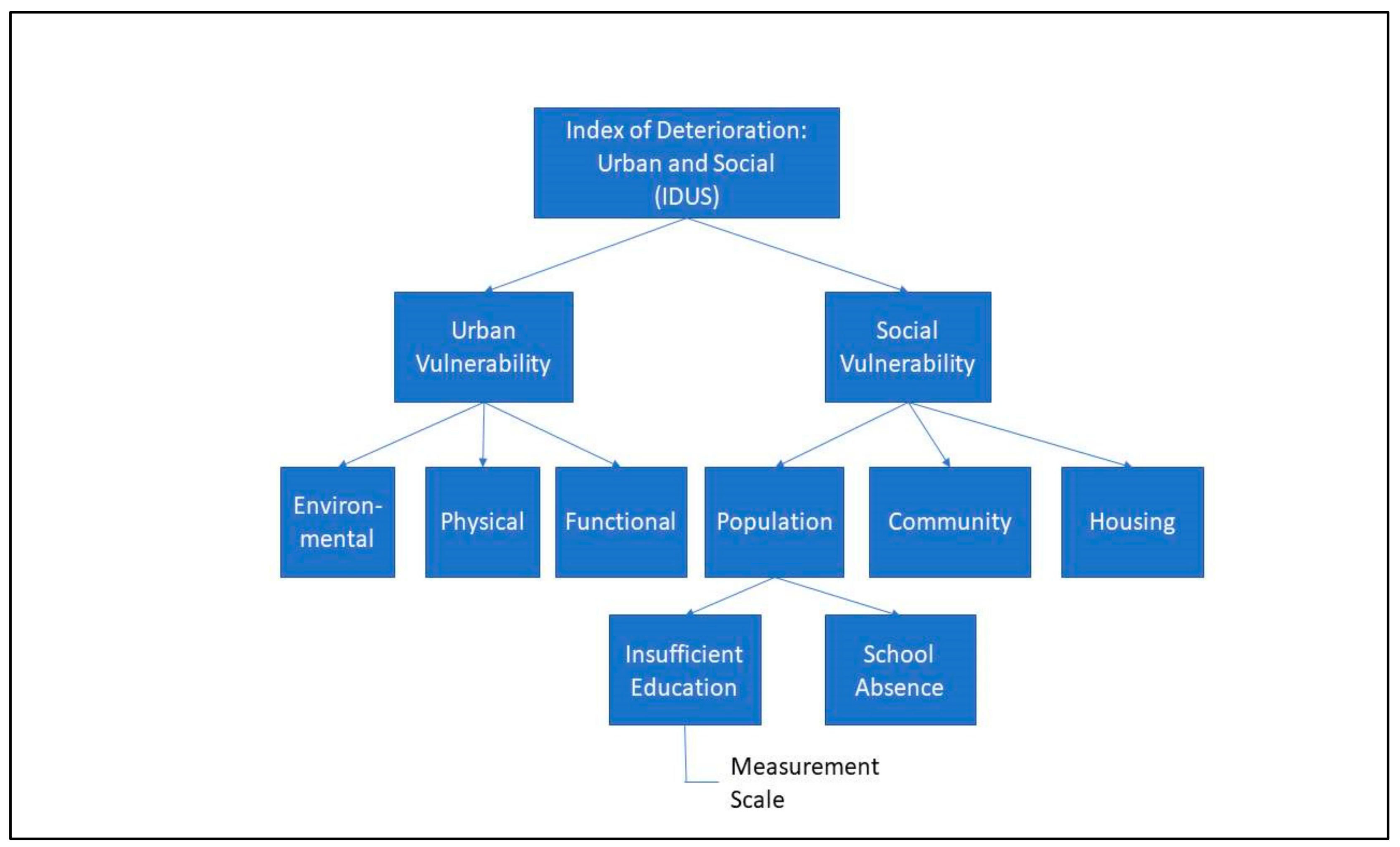
- IDUS (Ministerio de Desarrollo y Familia). Manual de Escalas Para la Cuantificación del Índice de Deterioro Urbano y Social (IDUS); Ministerio de Desarrollo y Familia: Santiago, Chile, 2019. [Google Scholar]
- Orton, A. Understanding rate of change. Math. Sch. 1984, 13, 23–26. [Google Scholar]
- Munda, G. Social Multi-Criteria Evaluation for a Sustainable Economy; Springer: Berlin, Germany, 2008. [Google Scholar]
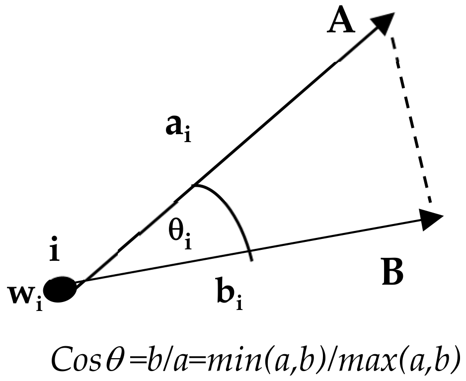
- Garuti, C. New advances of the compatibility index “G” in weighted environments. Int. J. Anal. Hierarchy Process 2016, 8, 514–536. [Google Scholar] [CrossRef]
- Garuti, C. (Ed.) A Set Theory Justification of Garuti’s Compatibility Index: Generalization of Jaccard Index Working within Weighted Environments; Nova Science Publishers: New York, NY, USA, 2022; Volume 30. [Google Scholar]


| Item | Source | Title | Contribution |
|---|---|---|---|
| 1 | Molinos-Senante et al. (2019) [10] Journal of Env. Management | Assessing the sustainability of small wastewater treatment systems: A composite indicator approach. | Quality of service for drinking water is assessed. If the max. quality CI score of 1 threshold is not reached, corrective action suggested. |
| 2 | Chung, et al. (2014) [13] World Journal of Gastroenterology | Can composite performance measures predict survival of patients with colorectal cancer? | Life expectancy evaluation composite indicator is based on its correlation of colon rectal cancer with life expectation. |
| 3 | Abdar et al. (2022) [14] Env. Sci. & Pollution Research | A composite index for assessment of agricultural sustainability: the case of Iran | The interval of standard meviation from the mean (ISDM) was applied for CI thresholds, e.g., unsustainable: CI < mean-standard deviation. |
| 4 | Corona-Sobrino et al. (2020) [7] PLOS One | Closing the gender gap at academic conferences: A tool for monitoring and assessing academic events | They use European Union gender set parameters as thresholds to create an action semaphore red/orange/green. |
| 5 | Bravo et al. (2023) [6] Natural Hazards | DRAI: a risk-based drought monitoring and alerting system in Brazil | The DRAI system generates alerts from statistical analysis based on the hazard, vulnerability, and risk indices following a normal distribution. An alert is generated whenever an index exceeds the value of the average of its historical series plus two SD. |
| 6 | Go, D. et al. [15] PLOS One | Development of the Korean Community Health Determinants Index (K-CHDI) | Authors develop a CI for health determinant index and validated it based on its correlation with life expectation data various communities. |
| 7 | Aguilar-Rivera, N. (2019) [11] Socio-Econ. Planning Sciences | A framework for the analysis of socio-economic and geographic sugarcane agro- industry sustainability | In this study, the normalized CI scale (0–1) is divided in four parts corresponding to the anchors high (1), medium (0.75), low (0.5), and very low (0.25). |
| 8 | Boggia et al. [16] Intl. Trans. in Oper. Research | Using accounting dataset for agricultural sustainability assessment through a multi-criteria approach: an Italian case study | Authors use the multiple reference point weak-strong composite indicators (MRP-WSCI) method, which allows decision-makers to set various reference levels for the indicators, such as aspiration levels (what is admissible) and aspiration levels (what is desirable), for each indicator. |
| 9 | Wang, et al. [17] Ecological Indicators | Vulnerability of mariculture areas to oil-spill stress in waters north of the Shandong Peninsula, China | To describe the spatial variations in vulnerability, the normalized values were divided into five classes by quartile distribution: extremely low, relatively low, medium, relative high, and extremely high. |
| 10 | Bansal, et al. [18] Modeling Earth Syst. and Env. | Evaluating urban flood hazard index (UFHI) of Dehradun city using GIS and multi-criteria decision analysis. | Authors use the natural breaks (or Jenks) classification method to identify very high, high, medium, and low flow hazard. Note: This method is best used with unevenly distributed data but not skewed toward either end of the distribution. |
| Levels of Risk Exposition According to BESIAK | |
|---|---|
| Reference point (Thresholds) | Risk Level |
| BESIAK total ≤ 300 | Low |
| 300 < BESIAK total ≤ 600 | Moderate |
| BESIAK total > 600 | High |
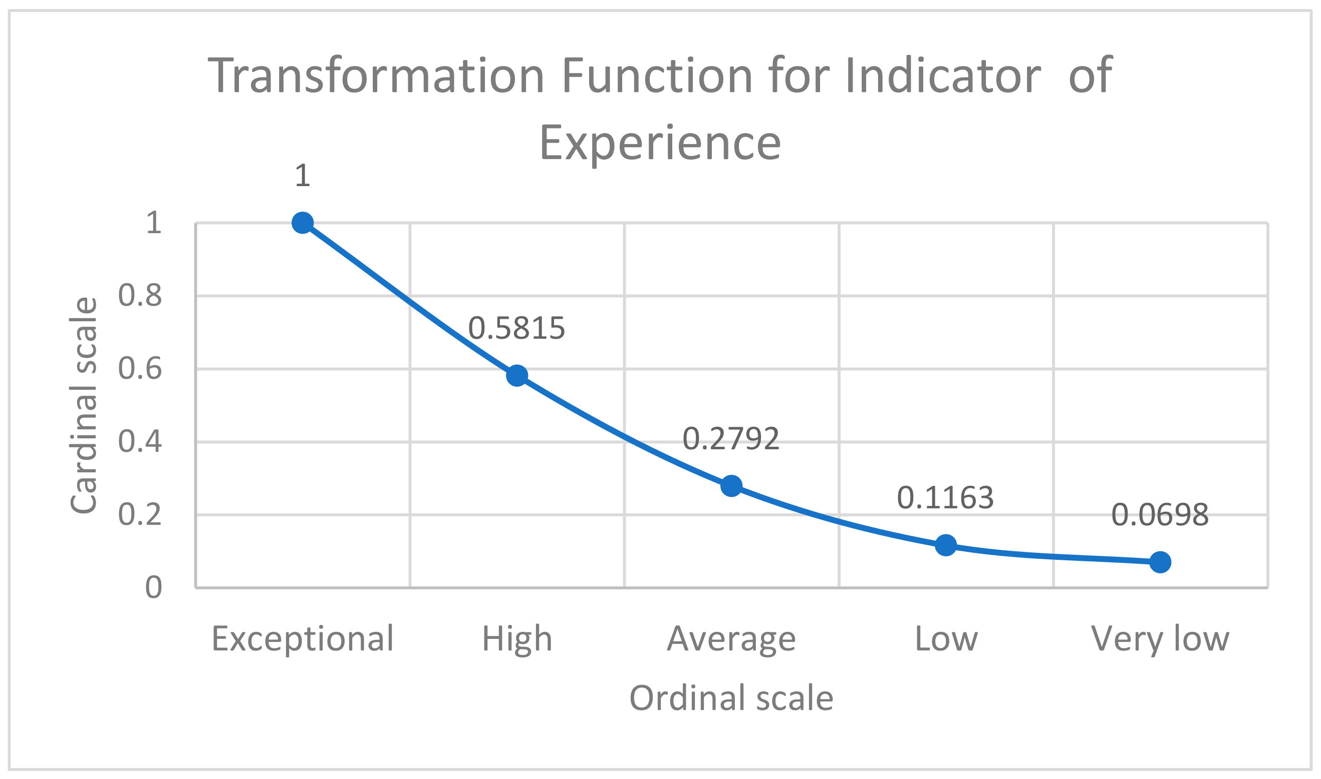
| Qualitative Scale | Quantitative Scale | Absolute Ratio Scale |
|---|---|---|
| Exceptional | 15 or more years of experience | 1.0000 |
| A lot | Between 8 to 14 years of experience | 0.5815 |
| Average | Between 4 and 7 years of experience | 0.2792 |
| Some | Between 1 and 3 years of experience | 0.1163 |
| Very little | Less than 1 year of experience | 0.0698 |
| Work Experience | Outstanding | A Lot | Average | Some | Very Little | Absolute Ratio Scale |
|---|---|---|---|---|---|---|
| Outstanding > 14 | 1 | a12 | a13 | a14 | a15 | 1 |
| A Lot (8–14) | 1 | a23 | a24 | a25 | 0.5815 | |
| Average (4–7) | 1 | a34 | a35 | 0.2792 | ||
| Some (1–3) | 1 | a45 | 0.1163 | |||
| Very little < 1 | 1 | 0.0698 |
| Scale Type | Invariant | Scale Threshold Example |
|---|---|---|
| Nominal | Bijective Function (one to one correspondence) | Car license plates ending in 3 and 4 (excluded from traffic circulation) |
| Ordinal | Monotone Function (increasing or decreasing) | Minimum grade: 4.0. (minimum grade for course approval) |
| Intervals (arbitrary zero) | Y = aX + b. (a, b > 0) (Straight line equation passing by b) | Temperature: 37 °C (maximum acceptable temperature to allow entry into a facility) |
| Ratio (dimensional, requires a known zero) | Y = aX. (a > 0) (Straight line equation passing by 0) | Speed: 50 km/h (maximum allowed speed) |
| Absolute Ratio (dimensionless, does not require a known zero) | Y = X (Identity Function) | Risk: 0.2485 (24.85%); maximum acceptable risk to implement a project in a given territory |
| Ordinal Scale of Insufficient Education Level | High | Moderate | Low | Very Low | Cardinal Scale of Insufficient Education Level |
|---|---|---|---|---|---|
| High | 1 | 2 | 7 | 9 | 1 |
| Moderate | 1/2 | 1 | 4 | 6 | 0.5524 |
| Low | 1/7 | 1/4 | 1 | 3 | 0.1736 |
| Very Low | 1/9 | 1/6 | 1/3 | 1 | 0.0847 |
| Ordinal |  | Cardinal | |||
| Terminal Criteria (Indicators) | LT(i) | WG(i) | LT(i) ∗ WG(i) |
|---|---|---|---|
| Exposure to greenhouse gas emission sources | 0.2999 | 0.5288 | 0.1586 |
| Exposure to pollutants (binary variable: 0–1) | 0 | 0.1454 | 0 |
| Exposure to noise emissions | 0.2999 | 0.1604 | 0.0481 |
| Exposure to micro garbage dump | 0.2494 | 0.1654 | 0.0413 |
| GT | - | 1.0 | 0.2480 |
| Metric Topology (Distance) | Order Topology (Compatibility) |
|---|---|
| D(a,b) = D(b,a) (Symmetry) | G(A,B) = G(B,A) |
| D(a,b) = 0 ⇔ a = b (Non null value) | G(A,B) = 1 ⇔ A = B |
| D(a,c) ≤ D(a,b) + D(b,c) (triangular inequality) | G(A,C) ≤ G(A,B) + G(B,C) |
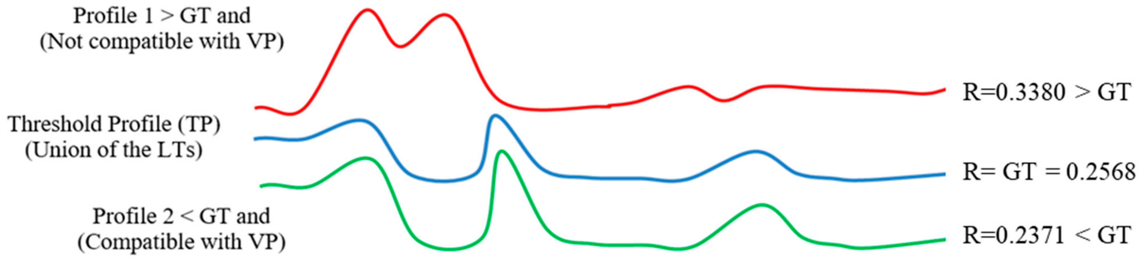
| lternative/Scenario | GT (Risks Model) | G | Result |
|---|---|---|---|
| A1 | A1 > GT Exceeds acceptable risk | G(A1;TP) < 85% Non compatible profile (not adjustable or too complex to be adjusted) | Rejected Alternative |
| A2 | A2 < GT Does not exceed acceptable risk | G(A2;TP) > 85% Compatible profile | Selectable alternative (no adjustment required) |
| A3 | A3 < GT Does not exceed acceptable risk | G(A3:TP) < 85% Non-compatible profile but possible to be adjusted | Alternative possible to be adjusted |
| A4 | A4 > GT Exceeds acceptable risk | G(A4;TP) > 85% Compatible profile | Alternative possible to be adjusted |
Disclaimer/Publisher’s Note: The statements, opinions and data contained in all publications are solely those of the individual author(s) and contributor(s) and not of MDPI and/or the editor(s). MDPI and/or the editor(s) disclaim responsibility for any injury to people or property resulting from any ideas, methods, instructions or products referred to in the content. |
© 2024 by the authors. Licensee MDPI, Basel, Switzerland. This article is an open access article distributed under the terms and conditions of the Creative Commons Attribution (CC BY) license (https://creativecommons.org/licenses/by/4.0/).
Share and Cite
Garuti, C.; Mu, E. A Rate of Change and Center of Gravity Approach to Calculating Composite Indicator Thresholds: Moving from an Empirical to a Theoretical Perspective. Mathematics 2024, 12, 2019. https://doi.org/10.3390/math12132019
Garuti C, Mu E. A Rate of Change and Center of Gravity Approach to Calculating Composite Indicator Thresholds: Moving from an Empirical to a Theoretical Perspective. Mathematics. 2024; 12(13):2019. https://doi.org/10.3390/math12132019
Chicago/Turabian StyleGaruti, Claudio, and Enrique Mu. 2024. "A Rate of Change and Center of Gravity Approach to Calculating Composite Indicator Thresholds: Moving from an Empirical to a Theoretical Perspective" Mathematics 12, no. 13: 2019. https://doi.org/10.3390/math12132019
APA StyleGaruti, C., & Mu, E. (2024). A Rate of Change and Center of Gravity Approach to Calculating Composite Indicator Thresholds: Moving from an Empirical to a Theoretical Perspective. Mathematics, 12(13), 2019. https://doi.org/10.3390/math12132019