
Computation of Green’s Function in a Strongly Heterogeneous Medium Using the Lippmann–Schwinger Equation: A Generalized Successive Over-Relaxion plus Preconditioning Scheme

Abstract
:1. Introduction
2. Methodology
2.1. L–S Equation for Green’s Function in a Medium with Slight Attenuation
2.2. Solution with Over-Relaxion plus Preconditioning
3. Choice of and
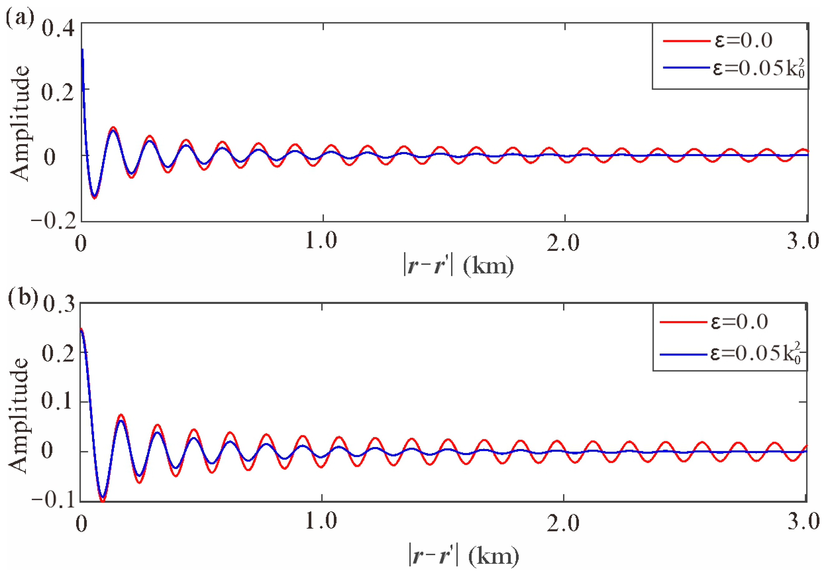
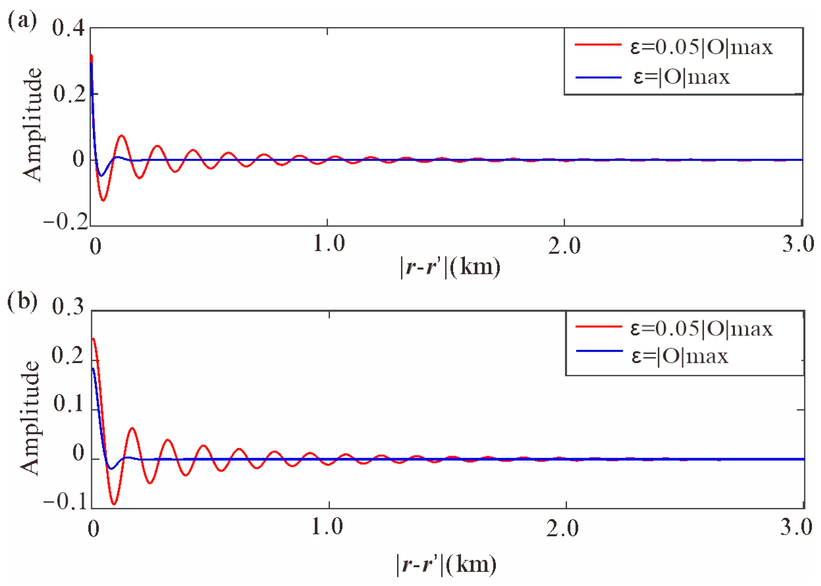
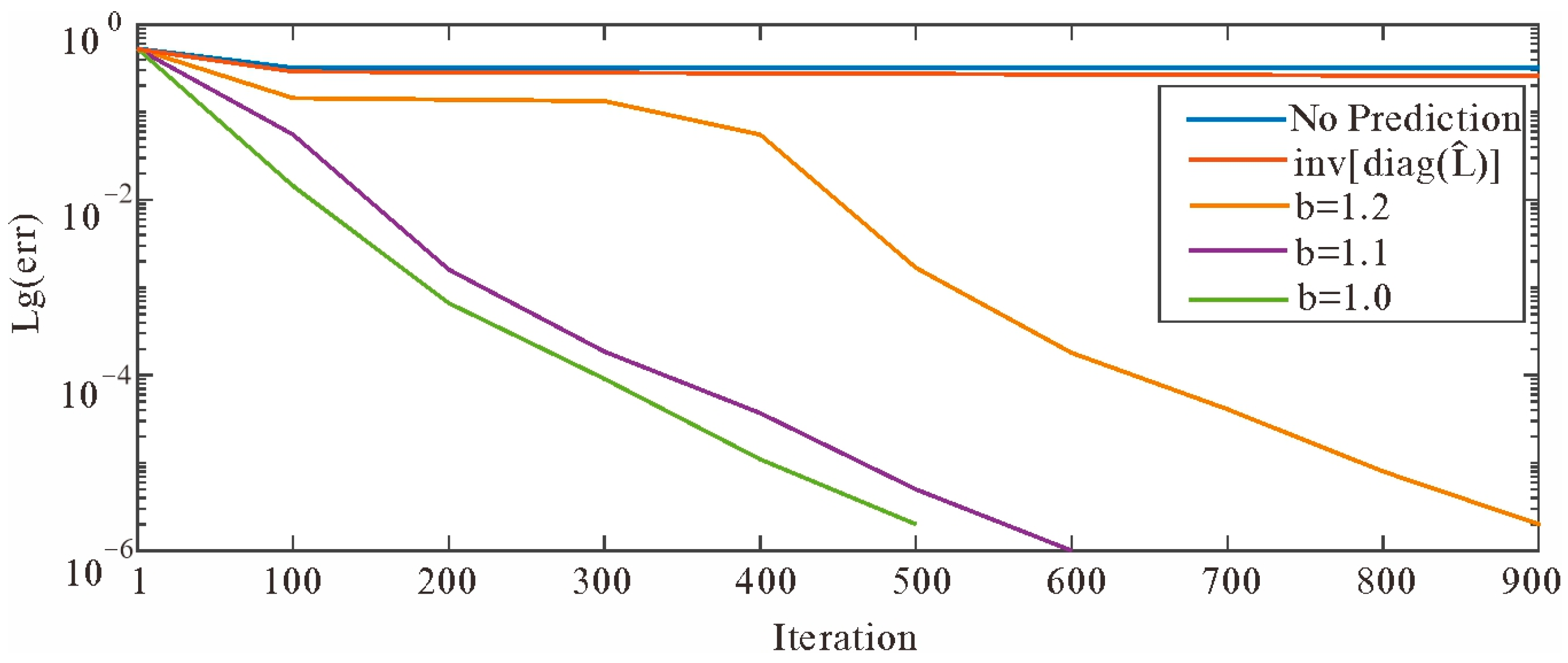
3.1. Influence of and Its Optimal Choice
3.2. Influence of and Its Optimal Choice
4. Numerical Test
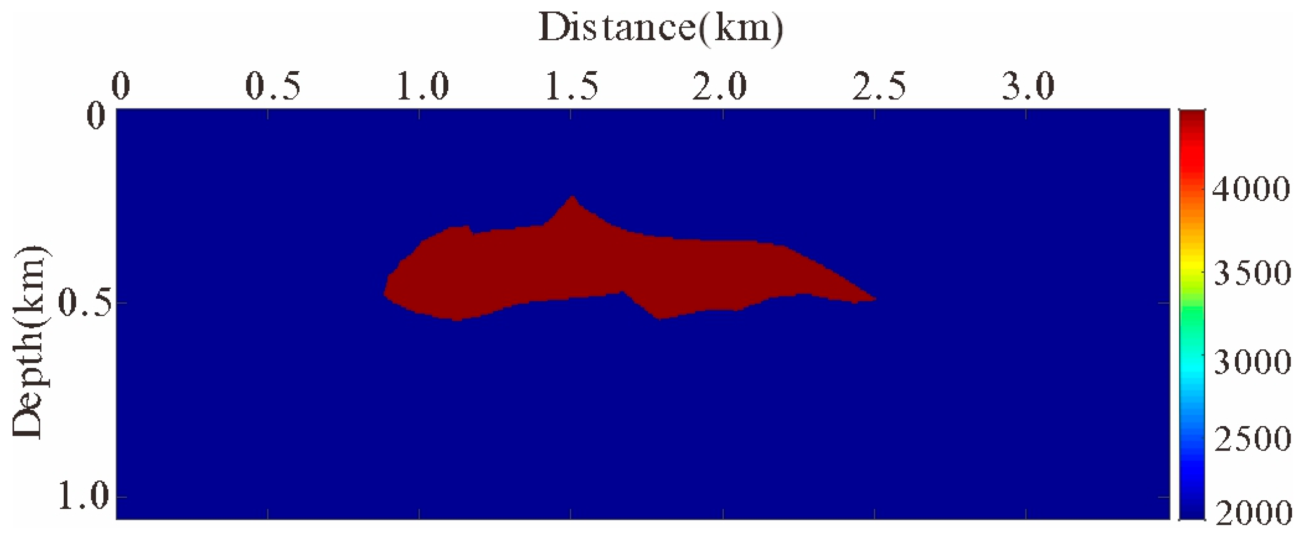
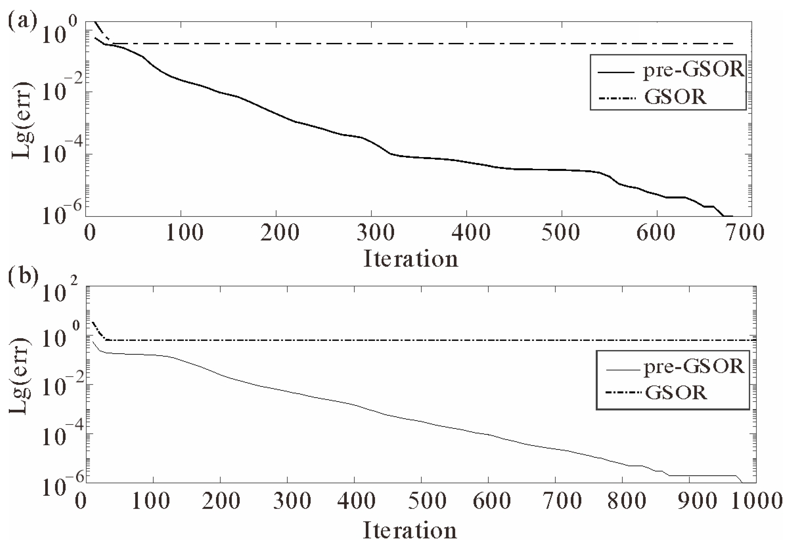
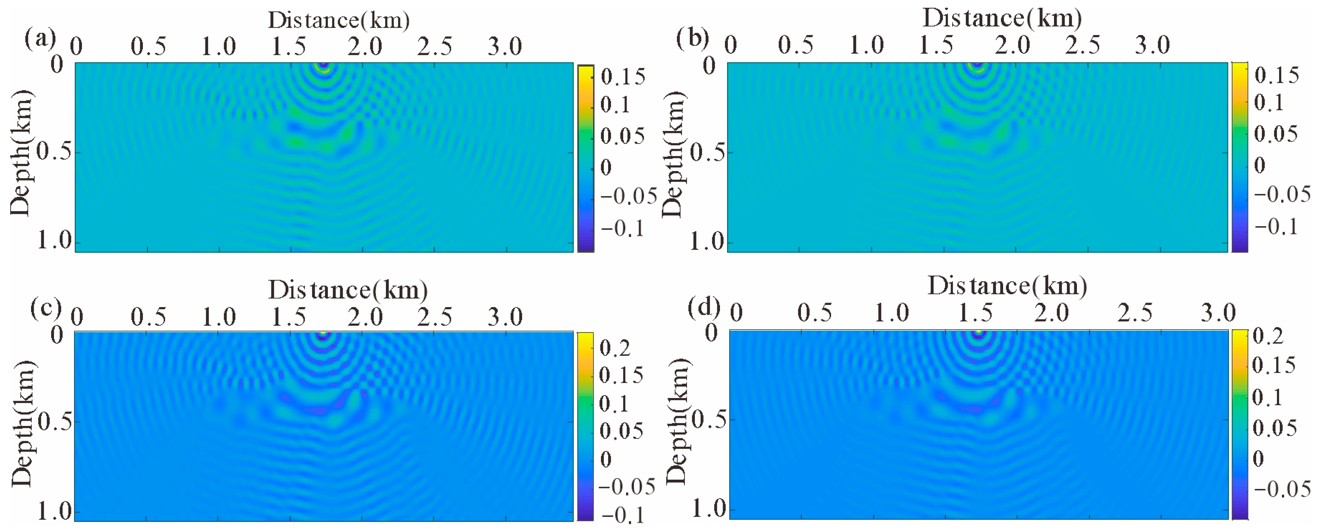
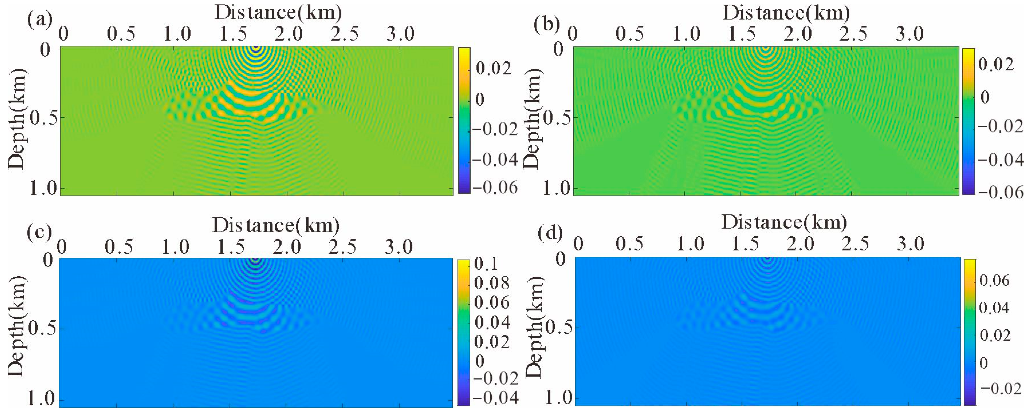
4.1. Single Salt Model
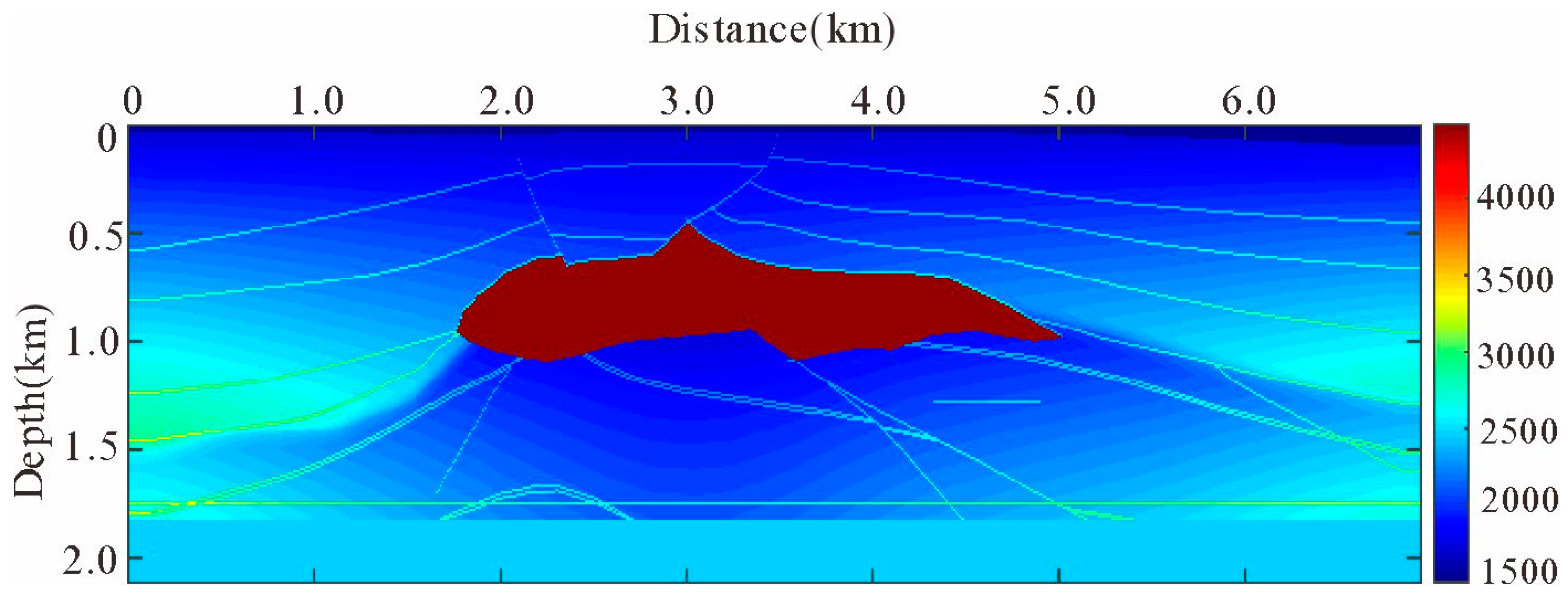
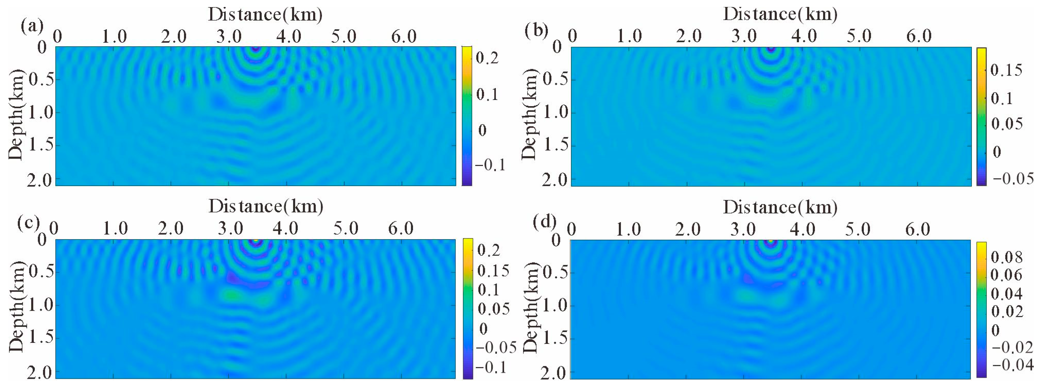
4.2. SEG/EAGE Salt Model
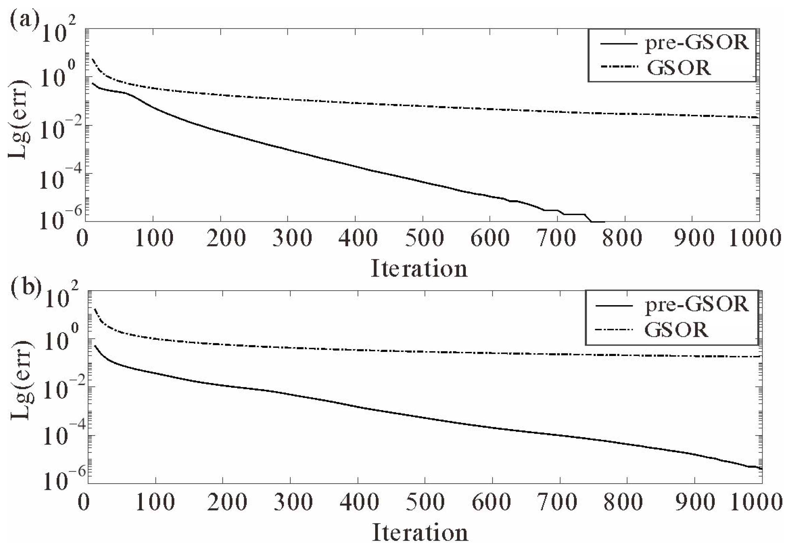
5. Analysis of Computation Efficiency and Memory Remand
6. Conclusions
Author Contributions
Funding
Data Availability Statement
Conflicts of Interest
References
- Sun, J. High-frequency asymptotic scattering theories and their applications in numerical modeling and imaging of geophysical fields: An overview of the research history and the state-of-the-art, and some new developments. J. Jilin Univ. (Earth Sci. Ed.) 2016, 46, 1231–1259. [Google Scholar]
- Cerveny, V. Seismic Ray Theory; Cambridge University Press: Cambridge, UK, 2001. [Google Scholar]
- Bleistein, N. Mathematical Methods for Wave Phenomena; USA Academic Press: Salt Lake City, UT, USA, 2012. [Google Scholar]
- Popov, M.M.; Semtchenok, N.M.; Popov, P.M.; Verdel, A.R. Depth migration by the Gaussian beam summation method. Geophysics 2010, 75, S81–S93. [Google Scholar] [CrossRef]
- Shi, X.; Sun, J.; Sun, H.; Liu, M.; Liu, Z. The time-domain depth migration by the summation of delta packets. Chin. J. Geophys. 2016, 59, 2641–2649. [Google Scholar]
- Sun, J. The history, the state of the art and the future trend of the research of Kirchhoff-type migration theory: A comparison with optical diffraction theory, some new result and new understanding, and some problems to be solved. J. Jilin Univ. (Earth Sci. Ed.) 2012, 42, 1521–1552. [Google Scholar]
- Huang, X.; Sun, H.; Sun, J. Born modeling for heterogeneous media using the Gaussian beam summation based Green’s function. J. Appl. Geophys. 2016, 131, 191–201. [Google Scholar] [CrossRef]
- Huang, X.; Sun, J.; Sun, Z. Local algorithm for computing complex travel time based on the complex eikonal equation. Phys. Rev. E 2016, 93, 043307. [Google Scholar] [CrossRef] [PubMed]
- Huang, X. Integral equation methods with multiple scattering and Gaussian beams in inhomogeneous background media for solving nonlinear inverse scattering problems. IEEE Trans. Geosci. Remote Sens. 2020, 59, 5345–5351. [Google Scholar] [CrossRef]
- Schuster, G.T. Reverse-time migration = generalized diffraction stack migration. In Proceedings of the SEG International Exposition and Annual Meeting, Salt Lake City, UT, USA, 6 October 2002. [Google Scholar]
- Schuster, G.T. Seismic Inversion; Society of Exploration Geophysicists: Yulsa, OK, USA, 2017. [Google Scholar]
- Zhang, G. Generalized Diffraction-Stack Migration. Ph.D. Thesis, The University of Utah, Salt Lake City, UT, USA, 2012. [Google Scholar]
- Zhang, G.; Dai, W.; Zhou, M.; Luo, Y.; Schuster, G.T. Generalized diffraction-stack migration and filtering of coherent noise. Geophys. Prospect. 2014, 62, 427–442. [Google Scholar] [CrossRef]
- Wu, R.S. Wave propagation, scattering and imaging using dual-domain one-way and one-return propagators. Pure Appl. Geophys. 2003, 160, 509–539. [Google Scholar] [CrossRef]
- Wu, R.; Xie, X.; Wu, X. One-way and one-return approximations (De Wolf approximation) for fast elastic wave modeling in complex media. Adv. Geophys. 2007, 48, 265–322. [Google Scholar]
- Innanen, K.A. Born series forward modelling of seismic primary and multiple reflections: An inverse scattering shortcut. Geophys. J. Int. 2009, 177, 1197–1204. [Google Scholar] [CrossRef]
- Jakobsen, M.; Wu, R. Renormalized scattering series for frequency-domain waveform modelling of strong velocity contrasts. Geophys. J. Int. 2016, 206, 880–899. [Google Scholar] [CrossRef]
- Huang, L.; Fehler, M.; Zheng, Y.; Xie, X.B. Seismic-Wave Scattering, Imaging, and Inversion. Commun. Comput. Phys. 2020, 28, 1–40. [Google Scholar]
- Jakobsen, M. T-matrix approach to seismic forward modelling in the acoustic approximation. Stud. Geophys. Geod. 2012, 56, 1–20. [Google Scholar] [CrossRef]
- Eftekhar, R.; Hu, H.; Zheng, Y. Convergence acceleration in scattering series and seismic waveform inversion using non-linear Shanks transformation. Geophys. J. Int. 2018, 214, 1732–1743. [Google Scholar] [CrossRef]
- Huang, K. A critical history of renormalization. Int. J. Mod. Phys. A 2013, 28, 1330050. [Google Scholar] [CrossRef]
- Jakobsen, M.; Wu, R. Accelerating the T-matrix approach to seismic full-waveform inversion by domain decomposition. Geophys. Prospect. 2018, 66, 1039–1059. [Google Scholar] [CrossRef]
- Jakobsen, M.; Wu, R.S.; Huang, X.G. Seismic waveform modeling in strongly scattering media using renormalization group theory. In Proceedings of the SEG International Exposition and Annual Meeting, Anaheim, CA, USA, 14 October 2018. [Google Scholar]
- Jakobsen, M.; Wu, R.; Huang, X. Convergent scattering series solution of the inhomogeneous Helmholtz equation via renormalization group and homotopy continuation approaches. J. Comput. Phys. 2020, 409, 109343. [Google Scholar] [CrossRef]
- Osnabrugge, G.; Leedumrongwatthanakun, S.; Vellekoop, I.M. A convergent Born series for solving the inhomogeneous Helmholtz equation in arbitrarily large media. J. Comput. Phys. 2016, 322, 113–124. [Google Scholar] [CrossRef]
- Huang, X.; Jakobsen, M.; Wu, R. On the applicability of a renormalized Born series for seismic wavefield modelling in strongly scattering media. J. Geophys. Eng. 2020, 17, 277–299. [Google Scholar] [CrossRef]
- Xu, Y.; Sun, J.; Shang, Y.; Meng, X.; Wei, P. The generalized over-relaxation iterative method for Lippmann-Schwinger equation and its convergence. Chin. J. Geophys. 2021, 64, 249–262. [Google Scholar]
- Xu, Y.; Sun, J.; Shang, Y. A parallel computation method for scattered seismic waves using Nyström discretization and FFT fast convolution. Chin. J. Geophys. 2021, 64, 2877–2887. [Google Scholar]
- Petryshyn, W.V. On a general iterative method for the approximate solution of linear operator equations. Math. Comput. 1963, 17, 1–10. [Google Scholar] [CrossRef]
- Kleinman, R.E.; Van den Berg, P.M. Iterative methods for solving integral equations. Radio Sci. 1991, 26, 175–181. [Google Scholar] [CrossRef]
- Golub, G.H.; Van Loan, C.F. Matrix Computations, 4th ed.; Johns Hopkins University Press: Baltimore, MD, USA, 2013. [Google Scholar]
- Hondori, E.J.; Mikada, H.; Goto, T.N.; Takekawa, J. A MATLAB Package for Frequency Domain Modeling of Elastic Waves. In Proceedings of the 75th EAGE Conference & Exhibition Incorporating SPE EUROPEC, London, UK, 10–13 June 2013. [Google Scholar]


| a | b | Frequency (f/Hz) | |||||
|---|---|---|---|---|---|---|---|
| 10 | 20 | 30 | 40 | 50 | 60 | ||
| 0.4 | 1.0 | 190 | 314 | >1000 | >1000 | >1000 | >1000 |
| 1.1 | 110 | 320 | >1000 | >1000 | >1000 | >1000 | |
| 1.2 | 105 | 360 | >1000 | >1000 | >1000 | >1000 | |
| 0.5 | 1.0 | 142 | 300 | 672 | >1000 | >1000 | >1000 |
| 1.1 | 129 | 306 | >1000 | >1000 | >1000 | >1000 | |
| 1.2 | 121 | 323 | >1000 | >1000 | >1000 | >1000 | |
| 0.6 | 1.0 | 183 | 303 | 459 | 585 | 713 | 733 |
| 1.1 | 150 | 303 | >1000 | >1000 | 799 | 785 | |
| 1.2 | 141 | 309 | >1000 | >1000 | >1000 | >1000 | |
| a | b | Frequency (f/Hz) | ||||
|---|---|---|---|---|---|---|
| 10 | 20 | 30 | 40 | 50 | ||
| 0.6 | 1.0 | 966 | >1000 | >1000 | >1000 | >1000 |
| 2.0 | 768 | >1000 | >1000 | 503 | 211 | |
| 3.0 | 755 | >1000 | >1000 | 931 | 225 | |
| 0.7 | 1.0 | 919 | >1000 | >1000 | >1000 | >1000 |
| 2.0 | 758 | 976 | 864 | 412 | 163 | |
| 3.0 | 757 | >1000 | >1000 | 605 | 172 | |
| 0.8 | 1.0 | 959 | >1000 | >1000 | >1000 | >1000 |
| 2.0 | 763 | 896 | 711 | 353 | 133 | |
| 3.0 | 760 | >1000 | >1000 | 439 | 135 | |
| Model | Pre-GSOR | FDFD | ||
|---|---|---|---|---|
| CPU Time (s) | Memory (M) | CPU Time (s) | Memory (M) | |
| Single Salt | 1.43 | 1.55 | 48.98 | 19.2 |
| SEG/EAGE Salt | 3.1 | 3.1 | 38.4 | 49.92 |
Disclaimer/Publisher’s Note: The statements, opinions and data contained in all publications are solely those of the individual author(s) and contributor(s) and not of MDPI and/or the editor(s). MDPI and/or the editor(s) disclaim responsibility for any injury to people or property resulting from any ideas, methods, instructions or products referred to in the content. |
© 2024 by the authors. Licensee MDPI, Basel, Switzerland. This article is an open access article distributed under the terms and conditions of the Creative Commons Attribution (CC BY) license (https://creativecommons.org/licenses/by/4.0/).
Share and Cite
Xu, Y.; Sun, J.; Shang, Y. Computation of Green’s Function in a Strongly Heterogeneous Medium Using the Lippmann–Schwinger Equation: A Generalized Successive Over-Relaxion plus Preconditioning Scheme. Mathematics 2024, 12, 2066. https://doi.org/10.3390/math12132066
Xu Y, Sun J, Shang Y. Computation of Green’s Function in a Strongly Heterogeneous Medium Using the Lippmann–Schwinger Equation: A Generalized Successive Over-Relaxion plus Preconditioning Scheme. Mathematics. 2024; 12(13):2066. https://doi.org/10.3390/math12132066
Chicago/Turabian StyleXu, Yangyang, Jianguo Sun, and Yaoda Shang. 2024. "Computation of Green’s Function in a Strongly Heterogeneous Medium Using the Lippmann–Schwinger Equation: A Generalized Successive Over-Relaxion plus Preconditioning Scheme" Mathematics 12, no. 13: 2066. https://doi.org/10.3390/math12132066
APA StyleXu, Y., Sun, J., & Shang, Y. (2024). Computation of Green’s Function in a Strongly Heterogeneous Medium Using the Lippmann–Schwinger Equation: A Generalized Successive Over-Relaxion plus Preconditioning Scheme. Mathematics, 12(13), 2066. https://doi.org/10.3390/math12132066