Integrated Optimization of Production Scheduling and Haulage Route Planning in Open-Pit Mines

Abstract

In mining, deposits are divided into blocks, forming the basis for open-pit mine planning, covering production and haulage route planning. Current studies often stage optimization and lack the consideration of road capacity, leading to suboptimal solutions. A novel approach integrates production scheduling and haulage route planning through a bilevel optimization model. The upper-level model integrates ore mining constraints to establish a mixed-integer production scheduling model, minimizing haulage costs. Spatiotemporal correlation constraints for block mining are determined using a two-stage algorithm. The lower-level model incorporates road capacity, forming a haulage route optimization model based on multicommodity network flow. A solution algorithm with a distance penalty strategy facilitates feedback between the upper and lower levels, achieving optimal solutions. Tested on a real open-pit coal mine with over 5 million blocks, this approach reduces haulage costs by 10.06% compared to stage optimization. Additionally, this approach allows for adjusting haulage demand in both temporal and spatial dimensions, effectively preventing road congestion. This study advances rational mining processes and enhances the efficiency of open-pit mining haulage systems.

1. Introduction

In the mining industry, deposits are subdivided into three-dimensional rectangular blocks to facilitate open-pit mining planning [1]. The ore grade of a block can be determined based on its mineral content, allowing for the assessment of its mining value and the identification of economic blocks. Depending on the variations in valuable mineral content, mined blocks are either transported as waste to nearby waste dumps or sent to processing plants for selective crushing and processing as ore [2].

Open-pit mine scheduling problems (OPMSPs) revolve around the management of various blocks, including mining scheduling (determining the timing and quantity of block extraction), dump scheduling (allocating blocks to waste dumps or processing plants), and haulage route planning (defining optimal transportation routes between loading and unloading locations) [3]. Mining and dump scheduling are often considered components of the broader production scheduling problem [4]. Typically, these processes are optimized in stages, with predefined mining schedules used to determine waste allocation or haulage routes planned based on predetermined dump schedules [5]. However, this approach has inherent limitations, as optimizing these components independently may result in suboptimal solutions for the entire mining complex [6].

Previous studies primarily focused on ore extraction as the main cost driver, with limited attention paid to material movement and handling [7]. In contrast, haulage costs account for up to half of the total operating costs in open-pit mining, amounting to millions of dollars [2]. When determining the optimal route between loading and unloading locations, it is crucial to consider global optimality rather than merely opting for the shortest route within the road network [8,9,10]. Despite this, existing pathfinding algorithms in mining operations often prioritize finding the shortest route without considering the capacity limitations of road segments [11,12]. This oversight can lead to congestion and excessive energy consumption during the scheduling process [13,14]. Therefore, achieving a globally optimal route, rather than simply the shortest route, is imperative.

Due to the limited road availability in open-pit mine networks, adjusting haulage routes alone may be insufficient to prevent road congestion issues, especially when operating under a predetermined production schedule. The production schedule, which dictates mining activities, volumes, and the choice of dump and processing plants, significantly impacts the selection and capacity utilization of haulage routes. Therefore, integrating production scheduling and haulage route planning is crucial for achieving a globally optimal solution in open-pit mining operations.

To address these issues, this study proposes an integrated optimization approach for production scheduling and haulage route planning in open-pit mines. The approach considers actual constraints such as the block mining sequence and road capacity. It formulates production scheduling optimization and haulage route planning as a bilevel optimization model to minimize haulage costs. Additionally, the study develops a solution algorithm incorporating a haulage distance penalty strategy.

1.1. Literature Review

The production scheduling problem in open-pit mines, particularly those involving large-scale blocks, is a challenging combinatorial optimization problem that is NP-hard. Samavati et al. [15] proposed a metaheuristic method based on local branching, which considers the minimum resource constraints within each period. Moreno et al. [16] enhanced their linear programming model with constraints on ore storage capacity to account for the effect of the waste dump on production scheduling. Fu, Asad, and Topal [7] presented a mixed-integer programming (MIP) model that addresses the open-pit mining and dump scheduling problem with the aim of maximizing the net present value. However, this model does not focus on the impact of haulage routes on costs. Elsayed et al. [6] introduced an evolutionary approach based on differential evolution, aiming to achieve high-quality solutions with reasonable computational costs.

The mining sequence of blocks plays a critical role in the design of open-pit mining schedules. It determines the spatiotemporal relationships involved in block extraction. This leads to the precedence constrained production scheduling problem (PCPSP), which involves scheduling tasks over a defined time horizon and assigning them to specific destinations. The scheduling must consider production capacity and precedence constraints and aim to maximize profits. However, solving the PCPSP, especially for practical-sized instances with hundreds of thousands or even millions of open-pit blocks, is nearly impossible [17].

To address this challenge, several studies have explored scenarios where block destinations are predetermined, aiming to find feasible solutions [3,18]. Additionally, clustering methods are used to scale down the problem and enhance computational traceability. Boland et al. [19] formulated the problem as a MIP model, applied aggregation to schedule mining, considered individual blocks for processing decisions, and solved it using the CPLEX solver. Several studies have focused on developing heuristic algorithms to address large-scale PCPSP problems, including genetic algorithms [20], tabu searches [21], and particle swarming algorithms [22].

The ultimate destination for material excavated in open-pit mining is either a waste dump or a processing plant. Choi et al. [23] introduced a new methodology for determining optimal truck haulage routes in large open-pit mines using multicriteria evaluation and least-cost path analysis. To address the truck–shovel allocation problem during the hauling process, Bakhtavar and Mahmoudi [11] proposed a two-stage model based on the shortest route. The first phase determines the amount of ore sent from the shovels, and in the second phase, the allocation of trucks to each shovel is determined. Several studies have examined the effects of road attributes on the hauling process. Choi and Nieto [24] developed a novel least-cost path algorithm to analyse haulage routes in open-pit mines. This algorithm considers terrain undulations and curves along the route, aiming to minimize truck transport time and fuel consumption. X. Li et al. [25] created an open-pit mine truck routing model that incorporates dynamic energy consumption, accounting for both road resistance and potential energy performed while lifting ore and rocks during haulage.

In summarizing previous studies, it is evident that these studies primarily focus on the block mining sequencing problem for open-pit mine production scheduling, with insufficient research conducted on haulage planning for ore or waste materials. Studies on open-pit mine haulage have primarily focused on optimizing truck–shovel allocation or analysing the effect of road attributes on the haulage process (e.g., elevation and road resistance). Additionally, most studies on route choice are based on the shortest route, and insufficient attention has been paid to road capacity.

1.2. Main Contributions

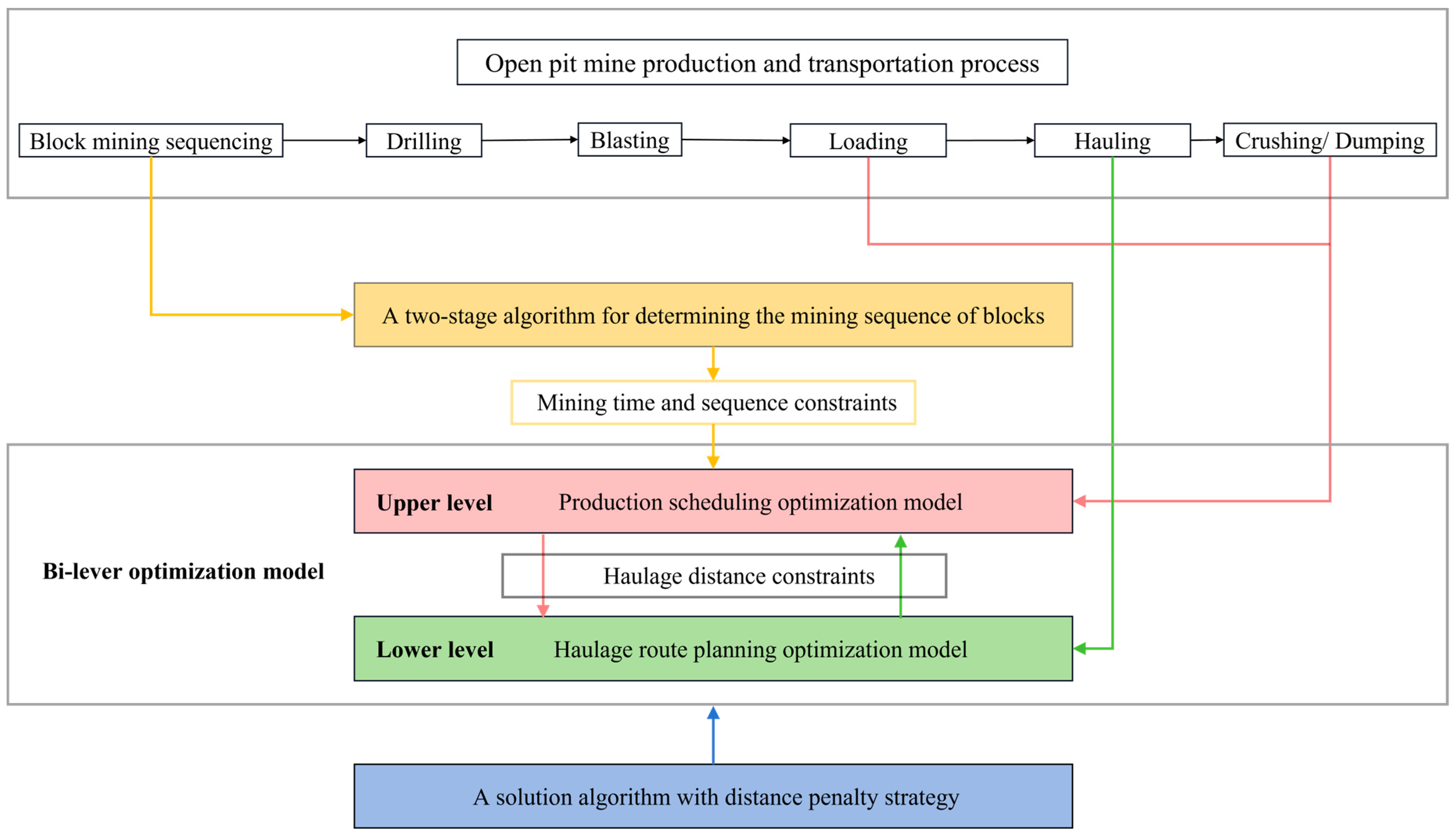
To address the shortcomings of stage optimization in production and transportation, and to enrich the methods for route planning in open-pit mines, this study investigates the integrated optimization of production scheduling and haulage route planning. The specific contributions are as follows:

(1) This study establishes the coupling relationship between the production scheduling problem and haulage route planning of open-pit mines by considering the haulage distance. A bilevel optimization model is constructed with the production scheduling optimization model as the upper-level model and the haulage route planning optimization model as the lower-level model, enabling the integrated optimization of the production scheduling problem and haulage route planning.

(2) To incorporate the spatiotemporal constraints of open-pit mining, a two-stage algorithm is proposed in the upper-level model to determine the mining sequence of blocks. In the lower-level model, road capacity is considered and a multicommodity flow model is developed to optimize the haulage routes.

(3) By designing a solution algorithm with a distance penalty strategy, a feedback mechanism between the upper- and lower-level models is established, enabling the solution of the bilevel optimization model for open-pit mine production scheduling and haulage route planning.

The structure of the remaining sections in this article is as follows: Section 2 presents an integrated optimization approach to production scheduling and haulage route planning. The proposed algorithm is described in Section 3, the computational results are presented in Section 4, and the conclusions are presented in Section 5.

2. Methodology

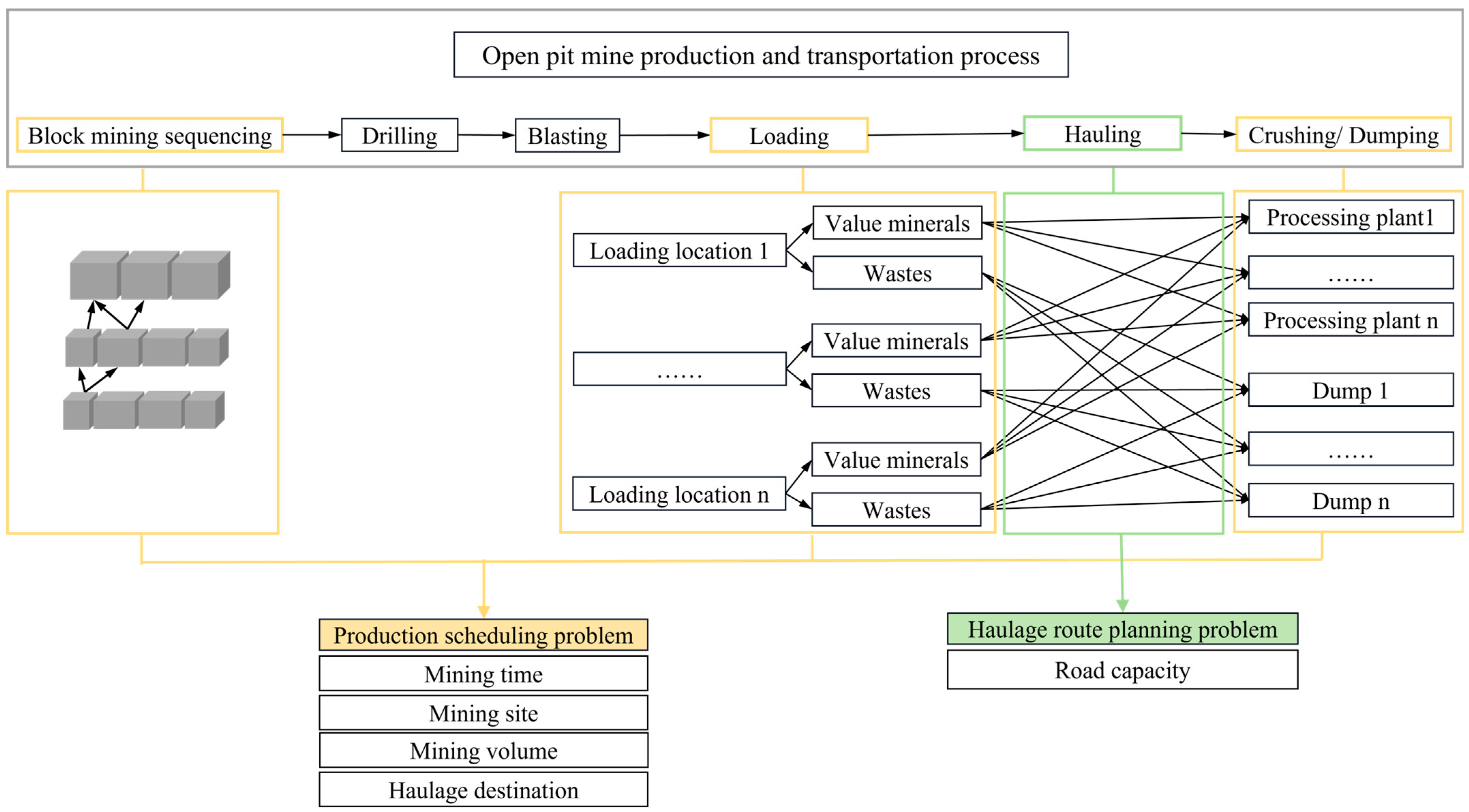
2.1. Problem Description

Open-pit mine production and transportation consist of block mining sequencing, drilling, blasting, loading, hauling, and crushing/dumping segments [11], as shown in Figure 1. After determining the spatiotemporal relationships of mining during the block mining sequencing phase, drilling and blasting operations are performed to form loading locations. Subsequently, mining trucks haul the mined ore or waste to either the processing plant or dump.

The first problem addressed in this study is the open-pit mine production scheduling problem, which involves determining when, where, and how much to mine, as well as where to deliver the mined material.

The second problem examined in this study is the haulage route planning problem, which specifically focuses on how road capacity affects route selection during hauling operations.

The third problem addressed in this study is achieving the integrated optimization of production scheduling and haulage route planning. The relationship between production scheduling and haulage route planning is characterized by coupling, where the production scheduling plan significantly influences the origin, destination, and volume of haulage route planning. Conversely, the specific routes selected also affect the haulage costs resulting from the production scheduling plan.

The research framework of this study is shown in Figure 2. To solve the open-pit mine production scheduling and haulage route planning problems, corresponding optimization models are constructed. The spatiotemporal correlation constraints in the production scheduling optimization model are determined by proposing a two-stage algorithm. To address the integrated optimization of production scheduling and haulage route planning, this study constructs a bilevel optimization model comprising a production scheduling optimization model and a haulage route planning optimization model. The coupling relationship between the upper- and lower-level models is expressed through haulage distance constraints. Moreover, a solution algorithm with a distance penalty strategy is proposed in Section 3 to solve the bilevel optimization model.

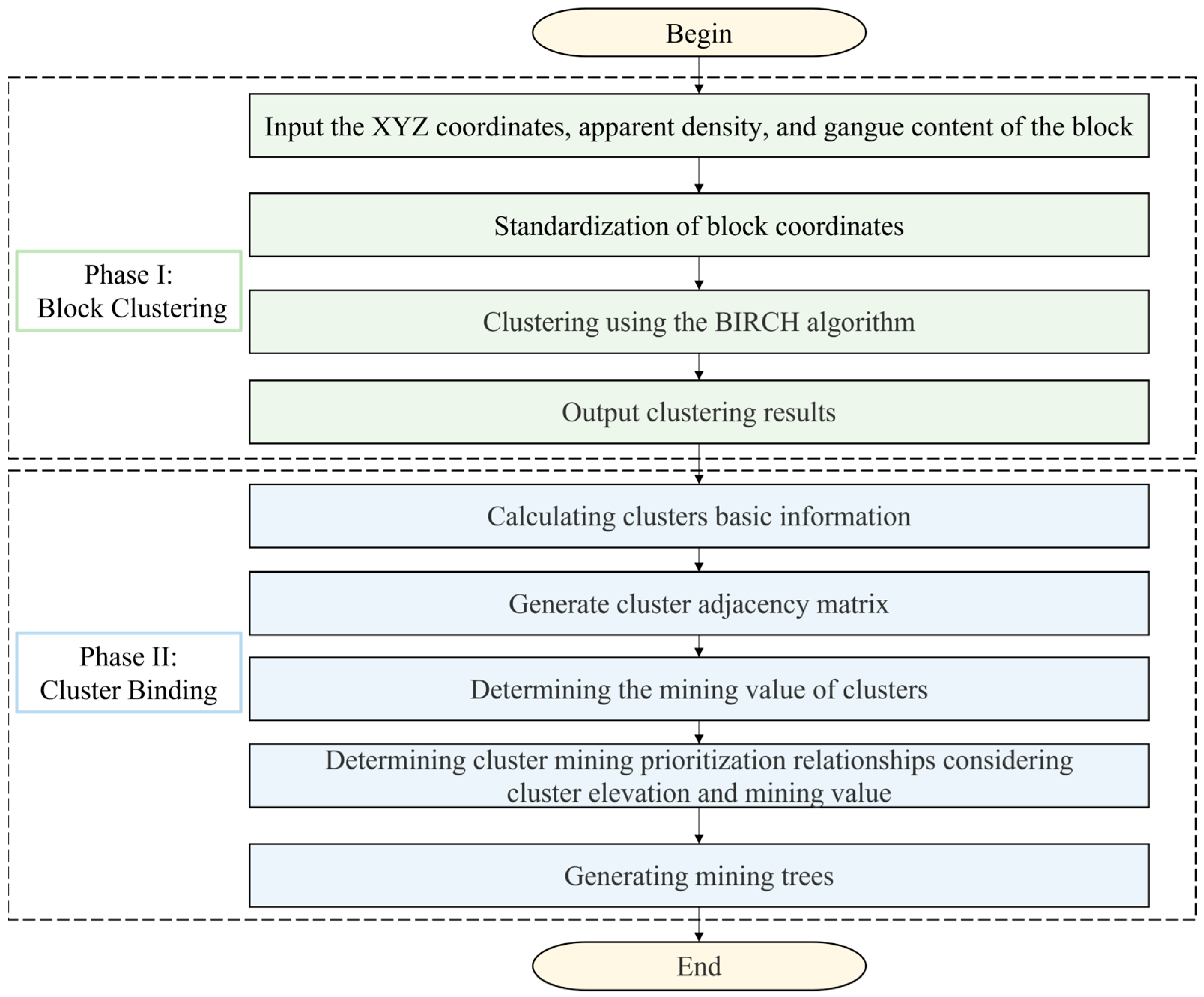
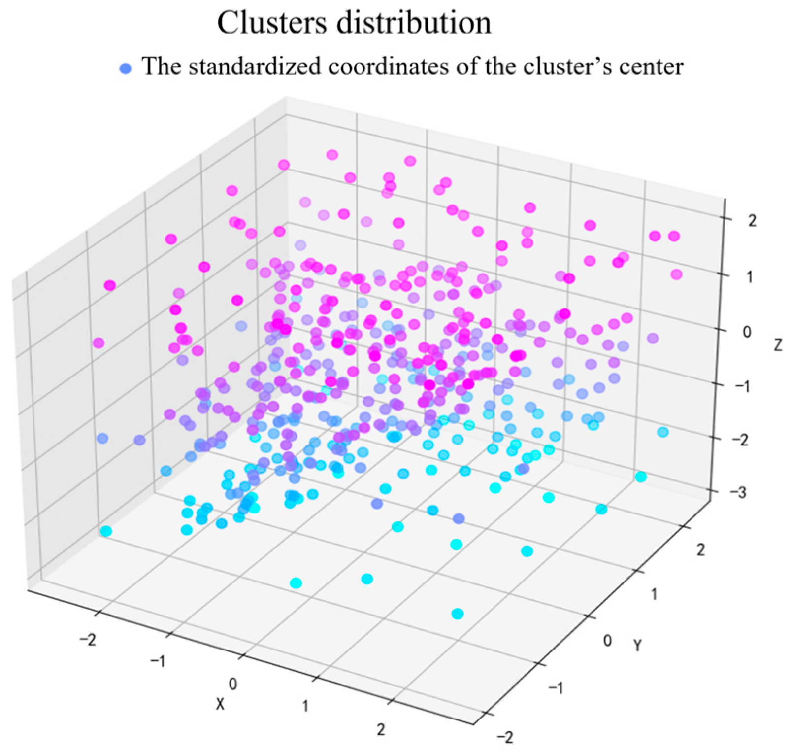
2.2. Block Mining Sequence

The mining sequence of the blocks determines the spatiotemporal constraints for production scheduling. However, open-pit mining often involves a large number of blocks, ranging from 2 million to 10 million. Optimizing production scheduling based on the original scale of blocks would result in optimization models that are difficult to solve or impractically time-consuming [3].

To address this, a two-stage preprocessing algorithm is proposed in this study to determine the mining sequence of blocks, aiming to reduce computation time and complexity. The algorithm flowchart is presented in Figure 3. The primary idea is to aggregate the blocks in the first stage, forming clusters to mitigate the difficulty in solving the optimization problem caused by the extensive number of decision variables [18,19]. In the second stage, these clusters are combined to form a mining tree, which determines the mining sequence [26]. Please refer to Algorithm 1 for detailed information.

(1)

Block clustering

Estimating the number of clusters formed by blocks in open-pit mines is challenging in practical scenarios. Unlike clustering algorithms such as k-means, which require the input of the number of clusters, the balanced iterative reducing and clustering using hierarchies (BIRCH) algorithm overcomes the need for predefined cluster numbers. The BIRCH algorithm uses a clustering feature tree to quickly cluster data, requiring three parameters: the branching factor $Br$, the spatial threshold, and the cluster count (optional). Algorithm details are available in Lang and Schubert [27] and Lorbeer et al. [28]. The BIRCH algorithm is known for its speed and ability to handle large datasets [27]. Therefore, it is employed for clustering blocks, aiming to reduce the dimensionality of decision variables.

(2)

Cluster binding

Once the blocks are aggregated into clusters, it is necessary to determine the mining sequence for each cluster. The fundamental tree algorithm is used to associate and bind the clusters. The binding process starts from the bottom up, starting with the block that has the highest average grade at the lowest level and finding the adjacent upper block. If these two blocks are found, they are bound together, and the process continues upward until no blocks are found above. Multiple mining trees are generated based on this process.

Algorithm 1. Two-stage algorithm for determining the mining sequence of blocks.
1	# Phase I: Block Clustering
2	Input: the XYZ coordinates, apparent density, and gangue content of the block
3	Standardization of block coordinates
4	clustering using the BIRCH algorithm
5	return cluster results and central coordinates of clusters
6	end
7	# Phase II: Cluster Binding
8	Input: cluster results, central coordinates of clusters, and block XYZ coordinate lengths
9	calculating cluster boundaries, mass, and valuable mineral content
10	generate cluster adjacency matrix
11	identifying clusters with positive valuable mineral content and establishing node set
12	calculating the mining value of clusters within the node set
13	calculating the level of clusters based on elevation
14	calculating the mining sequence of clusters within the node set
15	$\mathrm{establishing} \mathrm{a} \mathrm{set} seen$ to record occurrences of clusters
16	for each cluster $c$ within the node set:
17	$\mathrm{updating} \mathrm{set} seen$
18	$\mathit{if} \mathrm{the} \mathrm{current} \mathrm{cluster} \mathrm{within} \mathrm{the} \mathrm{set} seen$:
19	$\mathrm{set} \mathrm{the} \mathrm{mining} \mathrm{tree} tre{e}_c$ to empty
20	continue
21	$\mathrm{assign} \mathrm{the} \mathrm{current} \mathrm{cluster} \mathrm{to} \mathrm{the} \mathrm{set} \mathrm{of} \mathrm{adjacent} \mathrm{clusters} n\_set$
22	$\mathit{while} \mathrm{the} \mathrm{number} \mathrm{of} \mathrm{clusters} \mathrm{within} \mathrm{the} \mathrm{set} n\_set$ > 0:
23	$\mathrm{assign} \mathrm{the} \mathrm{clusters} \mathrm{from} \mathrm{the} \mathrm{set} n\_set$ $\mathrm{to} \mathrm{the} \mathrm{temporary} \mathrm{cluster} \mathrm{storage} \mathrm{set} tem\_set$
24	$\mathrm{add} \mathrm{the} \mathrm{clusters} \mathrm{from} \mathrm{the} \mathrm{set} tem\_set$$\mathrm{to} \mathrm{the} \mathrm{mining} \mathrm{tree} tre{e}_c$
25	$\mathrm{updating} \mathrm{set} seen$
26	$\mathrm{the} \mathrm{set} n\_set$ is reset to an empty set
27	$\mathit{for}\mathrm{each} \mathrm{cluster} \mathrm{within} \mathrm{the} \mathrm{set} tem\_set$:
28	$\mathrm{identify} \mathrm{clusters} \mathrm{from} \mathrm{the} \mathrm{neighboring} \mathrm{upper} \mathrm{level} \mathrm{and} \mathrm{exclude} \mathrm{those} \mathrm{that} \mathrm{have} \mathrm{already} \mathrm{been} \mathrm{recorded} \mathrm{in} \mathrm{the} \mathrm{set} seen$
29	$\mathrm{add} \mathrm{clusters} \mathrm{to} \mathrm{the} \mathrm{set} n\_set$
30	$\mathrm{remove} \mathrm{duplicate} \mathrm{clusters} \mathrm{from} \mathrm{the} \mathrm{set} n\_set$
31	return the mining tree
32	end

Algorithm 1 generates clusters composed of multiple blocks and mining trees determined by multiple clusters. The sequence of clusters within the mining tree represents the spatiotemporal development sequence during mining. The subsequent cluster $c$ can be mined only after mining the temporal and spatial precursor cluster $c^{\prime }$ (as shown by $c5$ and $c1$ in Figure 4). The subsequent integrated optimization of open-pit mine production scheduling and haulage route planning is based on these clusters and mining trees.

2.3. Production Scheduling Optimization Model

The upper-level model constructs a MIP model for the open-pit mine production scheduling problem. It is based on the following assumptions:

Assumption 1: 

All haulage vehicles are manually driven.

Assumption 2: 

Blocks within a cluster are mined simultaneously without prioritization.

Assumption 3: 

There is no priority relationship in the mining of clusters between different loading locations, but there is a priority relationship for the mining of clusters within the same mining tree.

The symbols used in the upper-level model are defined in

Table 1. Symbol table of the production scheduling optimization model.

Notation	Definition
Subscripts and sets
$t$	Mining time (month)
$o$	Loading location
$d$	Unloading location
$c$	Clusters
$T$	Mining time set
$O$	Loading location set
$D$	Unloading location set
$D_c$	Unloading location alternative set of clusters $c$
$Dv$	Processing plant set
$Cl$	Cluster set
$M_c$	Prioritized mining cluster set for cluster $c$$, M_c=\{m_{c1},\dots ,m_{cq}\}$
Input variable
$w_c$	The weight of the cluster $c$ (×104 t)
$w{v}_c$	The weight of value minerals contained in clusters $c$ (×104 t)
$h_{o,d}$	The elevation difference between loading location $o$ and unloading location $d$ (m)
$n_{c,o}$	Binary variable, if cluster $c$ is loaded at loading location $o$$, n_{c,o}=1$$, \mathrm{else} n_{c,o}=0$
$n{v}_d$	Binary variable, if unloading location $d$$\mathrm{is} \mathrm{the} \mathrm{processing} \mathrm{plant}, n{v}_d=1$$, \mathrm{else} n{v}_d=0$
$n{u}_{c,d}$	Binary variable, if cluster $c$ can be unloaded at unloading location $d$$, n{u}_{c,d}=1$$, \mathrm{else} n{u}_{c,d}=0$
$g_d$	The processing capacity at unloading location $d$ (×104 t/month)
$g_d^{\min }$	The minimum amount of value mineral required for the processing plant $d$ (×104 t)
$m_o$	The mining capacity at loading location $o$ (×104 t/month)
${\lambda }_1$	Haulage cost ($/104 t/m)
${\lambda }_2$	Unit material haulage change unit elevation cost ($/104 t/m)
Intermediate variable
$l_{o,d}$	Distance between loading and unloading locations (m)
Decision variables
$x_{t,c}$	Binary variable, if the cluster $c$ is mined in period $t$$, x_{t,c}=1$$, \mathrm{else} x_{t,c}=0$
$y_{t,c,d}$	The proportion of mined clusters $c$ hauled to unloading location $d$ in period $t$

.

Taking an overarching view of open-pit mining, where the mineral quantity remains constant and market fluctuations in mineral prices are not considered, the mine’s intrinsic value remains static. Within this context, the predominant factor leading to cost variations is the expenditure associated with haulage. Consequently, haulage costs emerge as a pivotal metric for evaluating the rationality of production scheduling in open-pit mining operations. Therefore, the optimization goal of the production scheduling model is to minimize haulage costs. The objective function takes into account the influence of differences in elevation and haulage distances on these costs and can be mathematically expressed as follows (Equation (1)).

$$\min {\displaystyle \sum _{t\in T}{\displaystyle \sum _{c\in Cl}{\displaystyle \sum _{o\in O}{\displaystyle \sum _{d\in D_c}{n}_{c,o}{w}_c{y}_{t,c,d}({\lambda }_1{l}_{o,d}+{\lambda }_2{h}_{o,d})}}}}$$

(1)

where $n_{c,o}$ is a binary variable indicating whether cluster $c$ is loaded at loading location $o$. $w_c$ is the weight of cluster $c$. $y_{t,c,d}$ is the proportion of cluster $c$ hauled to unloading location $d$ in period $t$. ${\lambda }_1$ is the haulage cost. ${\lambda }_2$ is the unit material haulage change unit elevation cost. $l_{o,d}$ is the distance from loading location $o$ of cluster $c$ to unloading location $d$. $h_{o,d}$ is the elevation difference between the loading location $o$ of cluster $c$ and the unloading location $d$. $T$ is the mining time set. $Cl$ is the cluster set. $O$ is the loading location set. $D_c$ is the unloading location alternative set of clusters $c$.

(1)

Unloading location selection constraints

When cluster $c$ is mined in period $t$, the ore or waste materials from cluster $c$ can be hauled to different unloading locations $d$, as expressed by Equation (2).

$$x_{t,c}\ge {\displaystyle \sum _{d\in D_c}{y}_{t,c,d}},\forall t\in T,\forall c\in Cl,$$

(2)

where $x_{t,c}$ is a binary variable indicating whether cluster $c$ is mined in period $t$.

(2)

Mining complete constraints

The sum of the proportions of haulage from cluster $c$ to each unloading location must be 1, indicating complete mining of the cluster. This constraint is expressed by Equation (3).

$${\displaystyle \sum _{\forall t\in T}{\displaystyle \sum _{d\in D_c}{y}_{t,c,d}}=1},\forall c\in Cl.$$

(3)

(3)

Mining time and sequence constraints

Clusters can be mined at different times, as expressed by Equation (4). Due to spatial constraints in open-pit mining, the subsequent cluster $c$ can only be mined once the spatial predecessor cluster $c^{\prime }$ has been mined. Based on the mining tree described in Section 2.2, it is possible to determine the prioritized mining cluster set for cluster $c$, i.e., $M_c$. Therefore, the mining sequence constraint can be expressed by Equation (5).

$${\displaystyle \sum _{t\in T}{\displaystyle \sum _{d\in D_c}{x}_{t,c}{y}_{t,c,d}=1}},\forall c\in Cl,$$

(4)

$$x_{t,c}\le {\displaystyle \sum _{t^{\prime }\in T}{\displaystyle \sum _{d\in D_{c^{\prime }}}{x}_{t^{\prime },c^{\prime }}{y}_{t^{\prime },c^{\prime },d}}},\forall t\in T,\forall c\in Cl,\forall c^{\prime }\in M_c.$$

(5)

(4)

Mining capacity constraints

The mining capacity is constrained by the quantity and capabilities of the mining equipment. Let $m_o$ denote the mining capacity at loading location $o$; the mining capacity constraint is represented by Equation (6).

$$0\le {\displaystyle \sum _{c\in Cl}{\displaystyle \sum _{d\in D_c}{n}_{c,o}{w}_c{y}_{t,c,d}}}\le m_o,\forall t\in T,\forall o\in O.$$

(6)

(5)

Processing plant value mineral requirement

To meet the quality requirements of valuable minerals (e.g., coal), any processing plant must fulfil the minimum amount requirement for valuable minerals, as expressed by Equation (7).

$$g_d^{\min }\le {\displaystyle \sum _{t\in T}{\displaystyle \sum _{c\in Cl}n{u}_{c,d}{w}_c{y}_{t,c,d}}},\forall d\in Dv,$$

(7)

where $Dv$ is the set of processing plants.

(6)

Value mineral content constraints

The amount of valuable minerals delivered to each processing plant from cluster $c$ cannot exceed the total content of valuable minerals in that cluster $c$. Let the variable $n{v}_d$ be a binary variable; if the unloading location $d$ is a processing plant, $n{v}_d=1$; otherwise, $n{v}_d=0$. Therefore, this constraint can be expressed by Equation (8).

$${\displaystyle \sum _{t\in T}{\displaystyle \sum _{d\in D_c}n{v}_d{w}_c{y}_{t,c,d}}}\le w{v}_c,\forall c\in Cl,$$

(8)

where $w{v}_c$ is the weight of the value minerals contained in cluster $c$.

(7)

Processing capacity constraints

The unloading locations are limited by the size of the site and the capacity of the processing equipment, resulting in a finite capacity for handling material. Let $g_d$ represent the processing capacity at unloading location $d$. This constraint can be expressed by Equation (9).

$$0\le {\displaystyle \sum _{c\in Cl}n{u}_{c,d}{w}_c{y}_{t,c,d}}\le g_d,\forall t\in T,\forall d\in D,$$

(9)

where $D$ is the set of unloading locations.

(8)

Haulage distance constraints

The haulage distance between loading and unloading locations can be determined by the ratio of the total haulage distance for the haulage task between loading and unloading locations to the total haulage volume, i.e., the unit material hauling distance, as expressed by Equation (10).

$$l_{o_k,d_k}=\frac{{\displaystyle \sum _{(i,j)\in E}{L}_{i,j}{z}_{i,j}^k}}{p_k},\forall k\in K,$$

(10)

where $i/j$ is the road node. $K$ is the set of haulage tasks in period $T$. $p_k$ is the haulage volume for haulage tasks $k$. $L_{ij}$ is the length of the road segment $\left(i,j\right)$. $z_{ij}^k$ is the haulage volume for haulage task $k$ on road segment $\left(i,j\right)$. $E$ is the set of road segments. $o_k/d_k$ is the loading/unloading location for haulage task $k$.

(9)

Variable constraints

The binary variables $x_{t,c}$ and continuous variables $y_{t,c,d}$ should, respectively, satisfy Equations (11) and (12).

$$x_{t,c}\in \left\{0,1\right\},\forall t\in T,\forall c\in Cl,$$

(11)

$$y_{t,c,d}\in \left[0,1\right],\forall t\in T,\forall c\in Cl,\forall d\in D_c.$$

(12)

2.4. Haulage Route Planning Optimization Model

Once the loading and unloading locations, mining time, and haulage volume are determined in the upper-level model for open-pit mining, the next step involves defining the specific haulage routes. Therefore, the lower-level model takes into account the limitation of road capacity and constructs a multicommodity network flow model to specify the routes between loading and unloading locations.

The following symbols in

Table 2. Symbol table of the haulage route planning optimization model.

Notation	Definition
Subscripts and sets
$i,j$	Road nodes
$k$	Haulage tasks
$K$	The set of haulage tasks in period $T$
$E$	The set of road segments
$V$	The set of road nodes
Input variables
$o_k/d_k$	Loading/unloading location for haulage task $k$
$p_k$	Haulage volume for haulage task $k$ (×104 t)
$u_{ij}$	Maximum road capacity of segment $\left(i,j\right)$ (×104 t/month)
$L_{ij}$	Length of road segment $\mathrm{Length} \mathrm{of} \mathrm{road} \mathrm{segment} \left(i,j\right)$ (m)
Decision variable
$z_{ij}^k$	Haulage volume for haulage task $k$ on road segment $\mathrm{on} \mathrm{road} \mathrm{segment} \left(i,j\right)$ (×104 t)

are used in the lower-level model.

Based on the decision variables $y_{t,c,d}$ of the upper-level model and the weight of clusters $w_c$, the set of haulage tasks $K$ is determined, as outlined in Algorithm 2. In transportation within open-pit mines, managers are most concerned with haulage costs, as these account for more than 50% of the total operating costs [2]. The haulage distance most directly reflects the situation of haulage costs. Therefore, to meet the haulage requirements and reduce haulage costs, the optimization objective of the haulage route planning optimization model is to minimize the haulage distance of haulage task $k$, as expressed by Equation (13).

$$\min {\displaystyle \sum _{(i,j)\in E}{\displaystyle \sum _{k\in K}{L}_{ij}{z}_{ij}^k}}$$

(13)

(1)

Network flow conservation constraints

For each haulage task, a quantity of $p_k$ of material is hauled from the loading location $o_k$, and no material is hauled to the loading location.

$${\displaystyle \sum _{j\in V}{z}_{o_{k}j}^k}-{\displaystyle \sum _{j\in V}{z}_{j{o}_k}^k}=p_k,\forall k\in K.$$

(14)

For each haulage task, a quantity of $p_k$ of material is hauled to the unloading location $d_k$, and no material is hauled out from the unloading location.

$${\displaystyle \sum _{j\in V}{z}_{d_{k}j}^k}-{\displaystyle \sum _{j\in V}{z}_{j{d}_k}^k}=-p_k,\forall k\in K,$$

(15)

The flow at the intermediate nodes of the road network is conserved, meaning the quantity of material hauled into and out of these nodes is equal for any haulage task.

$${\displaystyle \sum _{j\in V}{z}_{ij}^k}-{\displaystyle \sum _{j\in V}{z}_{ji}^k}=0,\forall k\in K,\forall i\in V,i\ne o_k,d_k,$$

(16)

(2)

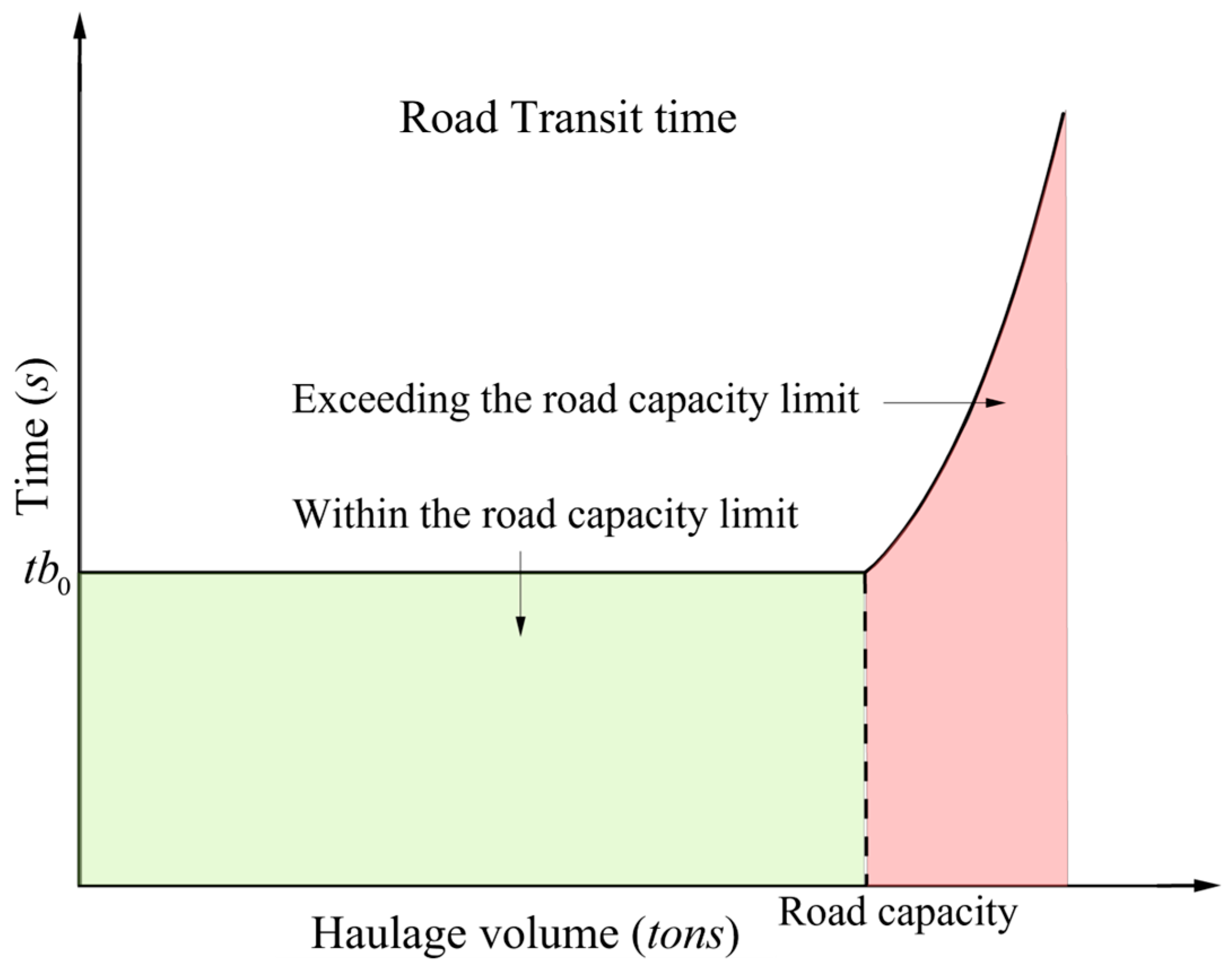
Road capacity constraints

For any haulage task, the haulage volume on each road segment must not exceed the road capacity of that segment.

$${\displaystyle \sum _{k\in K}{z}_{ij}^k}\le u_{ij},\forall (i,j)\in E,$$

(17)

where $u_{ij}$ is the maximum road capacity of segment $(i,j)$, representing the maximum amount of minerals that can be hauled per unit time. It can be determined by the number of mining trucks traveling through the segment per unit time and the load capacity of each truck.

(3)

Variable constraints

The haulage volume for any haulage task must not be negative.

$$z_{ij}^k\ge 0,\forall (i,j)\in E,\forall k\in K.$$

(18)

Algorithm 2. Updating haulage tasks
1	$\mathrm{Input}: \mathrm{upper}-\mathrm{level} \mathrm{model} \mathrm{decision} \mathrm{variable} y_{t,c,d}$$\mathrm{and} \mathrm{the} \mathrm{weight} \mathrm{of} \mathrm{cluster} w_c$
2	for each loading location $o$ of the set of loading locations $O$:
3	for each unloading location $d$ in the set of unloading locations $D$:
4	for each mining time $t$ in the set of mining times $T$:
5	$\mathit{for} \mathrm{each} \mathrm{of} \mathrm{the} \mathrm{clusters} \mathrm{of} \mathrm{the} \mathrm{cluster} \mathrm{set} Cl$:
6	if the cluster can be unloaded at $d$$\text{←}n{u}_{c,d}$
7	determining the proportion of clusters to be hauled
8	$\mathrm{determining} \mathrm{loading} \mathrm{locations} \mathrm{for} \mathrm{cluster} \mathrm{mining} \text{←}{n}_{c,o}$
9	If the mining haulage ratio ≠ 0 and the loading location ≠ 0:
10	determine the haulage volume $p$
11	add temporary haulage task $(t,o,d,p)$
12	$\mathrm{calculating} \mathrm{the} \mathrm{average} \mathrm{haulage} \mathrm{volume} \mathrm{for} \mathrm{loading} \mathrm{and} \mathrm{unloading} \mathrm{locations}, \mathrm{obtaining} \mathrm{haulage} \mathrm{tasks} (o,d,p)$ forming a set of haulage tasks $K$
13	return the set of haulage tasks $K$
14	end

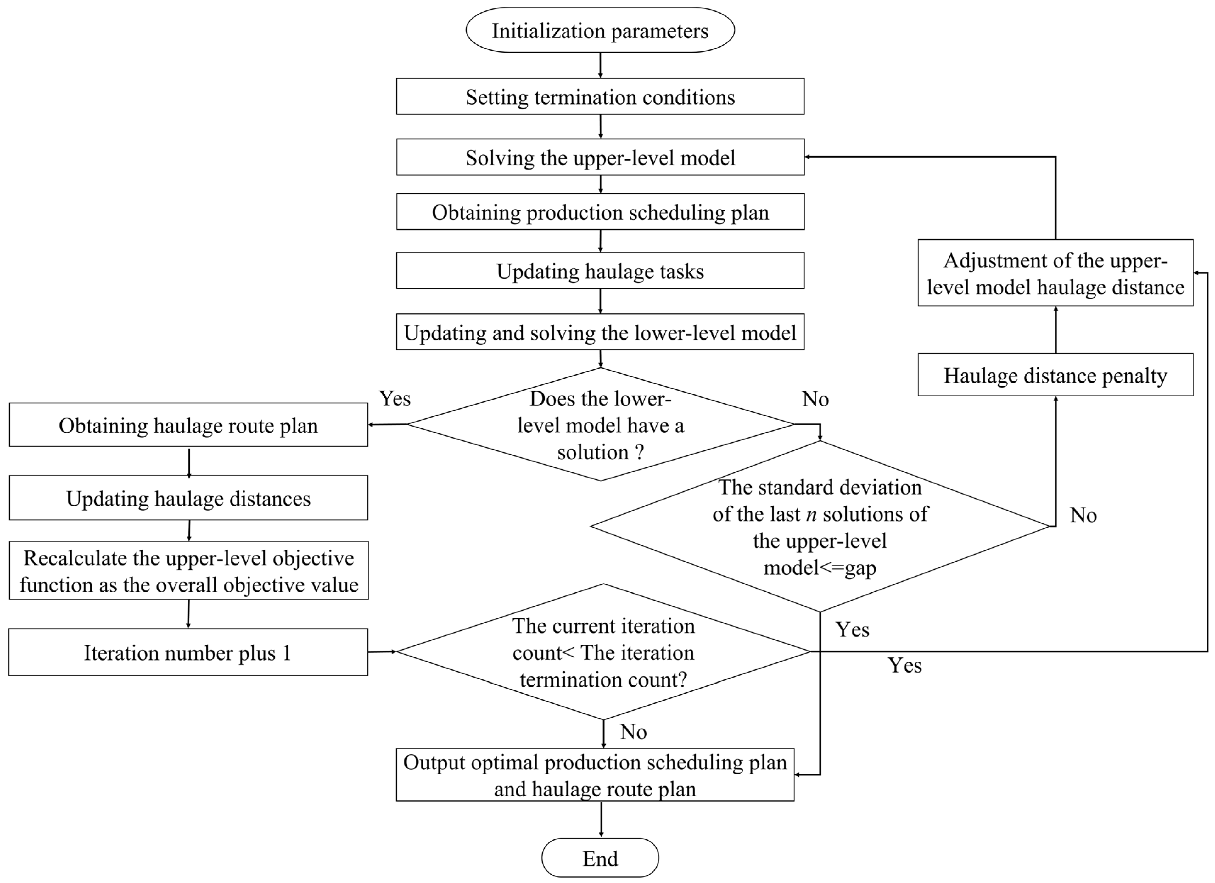
3. Solution Algorithm

The model developed in this study is a bilevel optimization model. To solve the model, a solution algorithm with a distance penalty strategy is designed, as illustrated in Figure 5. The algorithm establishes a feedback mechanism between the upper- and lower-level models through haulage distance feedback.

The upper-level model is solved using the initial haulage distance to obtain the production scheduling plan, which specifies the loading and unloading locations, mining time, and haulage volume. These results are subsequently passed into the lower-level model.

A failure of the lower-level model to generate feasible solutions indicates that the production scheduling plan determined by the upper-level model cannot find suitable routes for haulage tasks within the road capacity constraints. In such cases, it becomes necessary to readjust and resolve the production scheduling plan in the upper-level model.

To solve the model, designing an appropriate solving strategy is necessary. Distance-based solving strategies have been adopted in many studies [29,30]. In this study, haulage distance is a critical factor affecting material transport. Therefore, a distance penalty strategy is introduced in this study to help solve the bilevel model. The details of this strategy are as follows:

Distance increase penalty: Increase the distance by $u_{break}$ meters between the loading and unloading locations with the maximum haulage volume among all haulage tasks.

Distance decrease penalty: Decrease the distance by $u_{break}$ meters between the loading and unloading locations with the median haulage volume among all haulage tasks.

The purpose of the distance increase penalty is primarily to reduce the amount of material transported between loading and unloading locations where the maximum volume is being hauled. On the other hand, the distance decrease penalty aims to increase the haulage volume between loading and unloading locations with lower haulage volume, thereby allowing more unloading locations to be included in haulage route planning.

If the lower-level model cannot find a solution, haulage distance penalties are applied. The upper-level model is subsequently resolved to generate a new production scheduling plan. However, if the lower-level model finds a solution, it determines a haulage route plan specifying the routes between loading and unloading locations. The haulage distance is updated accordingly, and the upper-level objective function value is recalculated as the total objective value. This iterative solving process continues until the algorithm termination condition is met.

The recalculated upper-level objective function value, obtained after solving the lower-level model, represents the total objective value. This is because the upper-level objective value is determined by the initial haulage distance or the haulage distance updated with penalties. This value reflects only the haulage cost of the production scheduling plan at the current iteration. After successfully solving the lower-level model, the haulage distance is updated to reflect the actual distances between the loading and unloading locations. Therefore, recalculating the upper-level objective function value after solving the lower-level model provides the total objective value for the model.

Before each optimization in the lower-level model, it is necessary to determine the haulage task information, which includes the loading and unloading locations as well as the haulage volume. This determination is based on the decision variables $y_{t,c,d}$ of the upper-level model and the weights of the clusters $w_c$. The specific process is detailed in Algorithm 2. Similarly, before each optimization in the upper-level model, it is necessary to update the haulage distances based on the decision variables $z_{ij}^k$ of the lower-level model. The specific process is outlined in Algorithm 3.

Algorithm 3. Updating haulage distances
1	$\mathrm{Inputs}: \mathrm{lower}-\mathrm{level} \mathrm{model} \mathrm{decision} \mathrm{variable} z_{ij}^k$
2	for each haulage task $k$ in the set of haulage tasks $K$:
3	$\mathrm{determining} \mathrm{loading} \mathrm{location} o_k$$, \mathrm{unloading} \mathrm{location} d_k$$, \mathrm{and} \mathrm{haulage} \mathrm{volume} p_k$ for haulage task $k$
4	for each road segment in the road network segment set $E$:
5	calculating the total haulage distance for the haulage task $k$
6	$\mathrm{calculating} \mathrm{the} \mathrm{ratio} \mathrm{of} \mathrm{total} \mathrm{haulage} \mathrm{distance} \mathrm{to} p_k$
7	updating haulage distance
8	return haulage distances
9	end

The termination conditions of algorithms have various types, such as a fixed number of iterations, error or convergence criteria, time constraints, and so on [29,30,31]. To ensure the efficacy of the algorithm, two termination conditions are established. The first condition is based on the number of algorithm iterations, while the second condition is triggered when the standard deviation of the most recent $n$ solutions of the upper-level model falls below a specified gap value. The introduction of these termination conditions is primarily motivated by the finite nature of loading and unloading locations in open-pit mines. Additionally, considering the constraints of road capacity, the haulage route plans generated by the lower-level model are limited in feasibility. Setting this termination condition is essential for preventing excessive feedback and potential loops within the algorithm caused by distance updates.

4. Case Study

4.1. Data Description

A case study is conducted utilizing block data from an actual open-pit coal mine in China and road network data for a specific period. The open-pit coal mine consists of 5,828,219 blocks. The blocks are processed using the two-stage algorithm mentioned in Section 2.2 to determine the mining sequence. In this context, the BIRCH algorithm’s parameter $Br$ is set to 60, with a threshold of 0.6 [32]. This process ultimately results in the formation of 453 clusters, as depicted in Figure 6. From these, 20 mining trees are formed, and a total of 207 clusters are selected for mining.

The road network data are derived from the actual road network of an open-pit coal mine during a specific month in 2023. Road length and node coordinate information are extracted from the road network using QGIS and transformed into a topological road network. Elevation information for loading and unloading locations is obtained from online maps. The road network consists of 75 road segments, including 14 unloading locations, as shown in Figure 7. The open-pit mine comprises 20 mining trees, resulting in the selection of 20 loading locations from the existing loading locations and the designation of existing unloading locations as unloading locations. Additionally, four locations are chosen as processing plants, as outlined in

Table 3. The IDs for the loading/unloading locations.

Location Type	Set of IDs
Loading	1 3 4 5 7 8 9 10 11 18 19 22 23 24 28 32 35 36 37 38
Unloading	2 6 12 13 14 16 17 20 26 27 31 33 34 39 65
Processing plant	2 13 14 26

. In this case study, the initial distances between each loading and unloading location correspond to the shortest route distances.

The open-pit coal mine intends to extract a total of 31,346,700 tons of material, which includes 8,378,200 tons of coal.

Table 4. Loading location mining requirements and processing plant coal requirements.

Loading Location ID	Total Mining Volume (×104 t)	Coal Volume (×104 t)	Processing Plant ID	Coal Volume Requirements (×104 t)
1	991.38	110.24	2	70
3	421.22	39.59	13	120
4	196.31	19.42	14	50
5	342.50	25.42	26	180
7	118.39	25.53	-	-
8	84.63	10.74	-	-
9	53.27	16.49	-	-
10	32.31	7.55	-	-
11	30.95	25.72	-	-
18	51.73	36.80	-	-
19	24.95	21.57	-	-
22	83.64	55.21	-	-
23	31.42	26.20	-	-
24	188.94	39.63	-	-
28	45.63	3.00	-	-
32	80.47	70.16	-	-
35	91.24	74.15	-	-
36	129.86	120.45	-	-
37	126.63	105.60	-	-
38	9.18	4.35	-	-

provides the specific mining volumes for each loading location, as well as the coal volume required for processing plants to meet quality standards. The study period is 12 months. According to the mining design document provided by the coal mine operation and management company and relevant literature [33], set $m_o=4$ million tons per month, $g_d=4$ million tons per month, $u_{ij}=3.85$ million tons per month, ${\lambda }_1=1.69$ USD/10⁴ t/m, and ${\lambda }_2=1.41$ USD/10⁴ t/m.

The experiment is implemented using Python and the Gurobi solver (https://www.gurobi.com/ (accessed on 19 June 2024)). The distance penalty value $u_{break}$ is set to 500 m. The number of iterations for the first termination condition is set to 30. For the second termination condition, $n$ is set to 100 and the gap value is set to 0.001.

4.2. Results Analysis and Discussion

The iterative plot of the total objective value is represented in Figure 8. It is evident that the optimum is achieved at the third iteration, yielding an objective value of USD 20,885,328.25. Further details on the monthly haulage volumes at the loading and unloading locations can be found in Figure 9. The generated routes, totalling 39 routes, are presented in

Table 5. Haulage routes.

Route ID	Route	Route ID	Route
1	[1, 53, 67, 56, 57, 50, 17]	21	[19, 38, 71, 70, 72, 2]
2	[1, 53, 67, 58, 59, 52, 26]	22	[19, 38, 71, 70, 40, 43, 46, 57, 50, 17]
3	[3, 73, 74, 54, 56, 67, 58, 59, 52, 13]	23	[22, 66, 55, 67, 58, 59, 52, 13]
4	[3, 73, 74, 54, 56, 57, 50, 17]	24	[22, 66, 55, 67, 56, 57, 50, 17]
5	[3, 73, 74, 54, 56, 67, 58, 59, 52, 26]	25	[23, 69, 68, 67, 58, 59, 52, 13]
6	[4, 73, 74, 54, 56, 57, 50, 17]	26	[23, 69, 68, 67, 56, 57, 50, 17]
7	[4, 73, 74, 54, 56, 67, 58, 59, 52, 26]	27	[24, 69, 68, 67, 58, 59, 52, 13]
8	[5, 75, 76, 47, 49, 60, 63, 27]	28	[24, 69, 68, 67, 56, 57, 50, 17]
9	[7, 71, 70, 72, 2]	29	[28, 44, 46, 43, 40, 14]
10	[7, 71, 70, 40, 43, 46, 57, 50, 17]	30	[28, 44, 46, 57, 50, 17]
11	[8, 45, 44, 46, 43, 40, 70, 72, 2]	31	[32, 76, 47, 31]
12	[8, 45, 44, 46, 43, 40, 14]	32	[35, 43, 40, 14]
13	[8, 45, 44, 46, 57, 50, 17]	33	[35, 43, 46, 57, 50, 17]
14	[9, 45, 44, 46, 43, 40, 70, 72, 2]	34	[36, 68, 67, 58, 59, 62, 61, 64, 12]
15	[9, 45, 44, 46, 57, 50, 17]	35	[36, 68, 67, 56, 57, 46, 43, 40, 14]
16	[10, 54, 56, 67, 58, 59, 52, 13]	36	[37, 53, 67, 58, 59, 52, 13]
17	[10, 54, 56, 57, 50, 17]	37	[37, 53, 67, 56, 57, 50, 17]
18	[11, 74, 54, 56, 57, 50, 17]	38	[38, 71, 70, 72, 2]
19	[11, 74, 54, 56, 67, 58, 59, 52, 26]	39	[38, 71, 70, 40, 43, 46, 57, 50, 17]
20	[18, 60, 49, 48, 33]	-	-

.

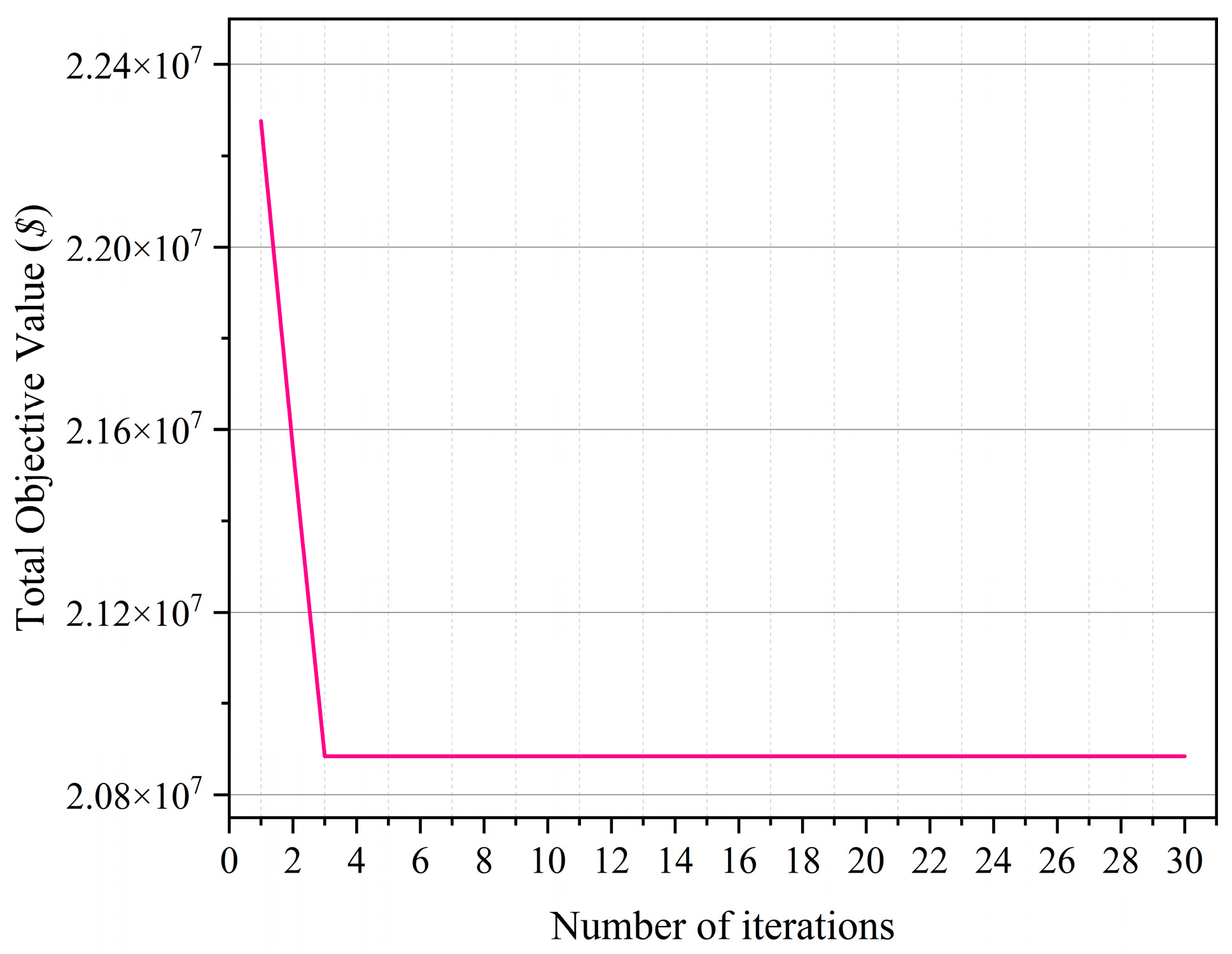
4.2.1. Comparison of the Optimized Results

To compare the effects of optimization, the traditional approach of selecting loading and unloading locations based on the shortest distance is utilized for production scheduling and haulage route planning (referred to as the staged optimization approach). The results are presented in

Table 6. Results comparison.

	Staged Optimization Approach	Integrated Optimization Approach	Improvement
Total objective value (USD)	23,221,832.77	20,885,328.25	−10.06%
The number of segments exceeding road capacity	5	0	−5

. To reflect the additional costs resulting from segments exceeding road capacity, the widely used BPR function road resistance model is adopted as the comprehensive road resistance function for open-pit mines [34,35], as shown in Equation (19). In this study, this model clarifies the relationship between the total material volume of mining truck haulage on road segments and the road capacity. When the haulage volume on a road segment is within the road capacity, trucks can move freely without congestion, resulting in free flow. In this scenario, assuming the trucks are traveling at the speed limit of the road segment (usually set at 30 km/h), the travel time for the trucks on the segment is fixed. However, when the haulage volume exceeds the road capacity, trucks may experience congestion, queues, or detours, leading to a reduction in speed and an increase in transit time, as shown in

Table 7. Extra transit time for average monthly haulage volume on road segments.

Segment Exceeding road Capacity	The Haulage Volume (×104 t)	Transit Time (s)	Transit Time Considering Road Capacity (s)	Extra Time (s)
(67, 58)	414.86	59.33	70.53	11.20
(58, 59)	414.86	28.47	33.84	5.37
(59, 52)	414.86	47.84	56.87	9.03
(57, 50)	386.70	213.06	243.42	30.36
(50, 17)	386.70	5.63	6.43	0.80
Total	2017.98	354.33	411.09	56.76

. Therefore, the relationship between transit time and haulage volume on the road segment $ij$ in this study can be shown in Figure 10.

$$t{b}_{ij}=t{b}_0[1+\alpha {(\frac{p_{ij}}{u_{ij}})}^{\beta }],$$

(19)

where $t{b}_{ij}$ is the travel time for trucks on road segment $ij$. $t{b}_0$ is the linear travel time based on the length of the road segment, i.e., $t{b}_0=L_{ij}/v$. The speed limit of the road segment for open-pit mines is 30 km/h, i.e., $v=8.33$ m/s. $p_{ij}$ is the haulage volume on road segment $ij$. $\alpha$ and $\beta$ are constant values of 0.13 and 4 [34,35,36], respectively. By converting the units of haulage cost (1.69 USD/10⁴ t/m) and speed (8.33 m/s), the haulage cost per unit time (i.e., transit time cost) becomes 14.08 USD/10⁴ t/s. Since the more precise haulage cost per unit time is not the focus of this paper, the haulage cost per unit time in this study is fixed and does not change with reduced speed.

Segment Exceeding road Capacity	The Haulage Volume (×104 t)	Transit Time (s)	Transit Time Considering Road Capacity (s)	Extra Time (s)
(67, 58)	414.86	59.33	70.53	11.20
(58, 59)	414.86	28.47	33.84	5.37
(59, 52)	414.86	47.84	56.87	9.03
(57, 50)	386.70	213.06	243.42	30.36
(50, 17)	386.70	5.63	6.43	0.80
Total	2017.98	354.33	411.09	56.76

Therefore, the additional cost resulting from segments exceeding road capacity during the mining cycle can be calculated to be USD 3,830,147.07 by multiplying the total haulage volume for road segments, the extra transit time, and the transit time cost.

Table 6 shows that the total haulage cost of the staged optimization approach is USD 23,221,832.77, whereas the total haulage cost of the integrated optimization approach is USD 20,885,328.25, representing a decrease of 10.06%. This demonstrates that implementing an integrated optimization of production scheduling and haulage route planning effectively reduces haulage costs. Additionally, the staged optimization approach resulted in five segments exceeding the road capacity limit. In contrast, the integrated optimization approach considers road capacity constraints, resulting in no segments exceeding the road capacity limits. This is accomplished by changes to the haulage volume and some haulage routes. For further details on the haulage routes, please refer to Section 4.2.3.

In conclusion, this study provides an efficient approach for the integrated optimization of production scheduling and haulage route planning in open-pit mines. It also offers a novel approach for mitigating road congestion and reducing costs in such mining operations.

4.2.2. Impact of the Distance Penalty Strategy

To illustrate the impact of the distance penalty strategy, this section discusses and analyses the solving process of the upper- and lower-level models, as depicted in Figure 11.

In this experiment, the algorithm terminates after 30 iterations. However, the production scheduling plan generated by the upper-level model may cause infeasibility issues for the lower-level model. Therefore, the upper-level model may need to be resolved with distance penalties, resulting in more than 30 iterations being required for the upper-level model to meet the termination condition.

Throughout the iterative solving process, the upper-level model completes a total of 72 iterations, as shown in Figure 11. Among these, 42 instances indicate the infeasibility of the lower-level model, prompting a resolve with distance penalties. The upper-level objective value continuously increases, followed by fluctuations. This pattern can be attributed to the initial iterations, where the production scheduling plan determined by the upper-level model violates road capacity constraints while solving the lower-level model, resulting in distance penalties and an increase in the objective value. Subsequently, due to the relatively simple structure of the open-pit mine road network, there are limited feasible routes satisfying road capacity requirements, and after each lower-level model solving iteration, the haulage distance is updated to reflect the actual haulage distance. As a result, the upper-level objective value continues to fluctuate after the optimal solution is found.

Moreover, the number of iterations to obtain the optimal value of the total objective (obtained in the 3rd iteration; see Figure 8) is different from the number of iterations to obtain the optimal value of the low-level model (obtained in the 22nd iteration; see Figure 11). This discrepancy arises from variations in haulage costs influenced by differing elevations between loading and unloading locations, as well as fluctuations in the number of haulage tasks determined by the lower-level model in each iteration. This further highlights the failure of staged optimization in achieving a superior global optimum for production scheduling and haulage route planning. Therefore, it is crucial to pursue integrated optimization strategies.

In conclusion, the lower-level model becomes infeasible without a distance penalty strategy. By implementing the distance penalty strategy, more effective distance feedback between the upper- and lower-level models is achieved, facilitating the solution of the integrated optimization bilevel model for open-pit mining production scheduling and haulage route planning.

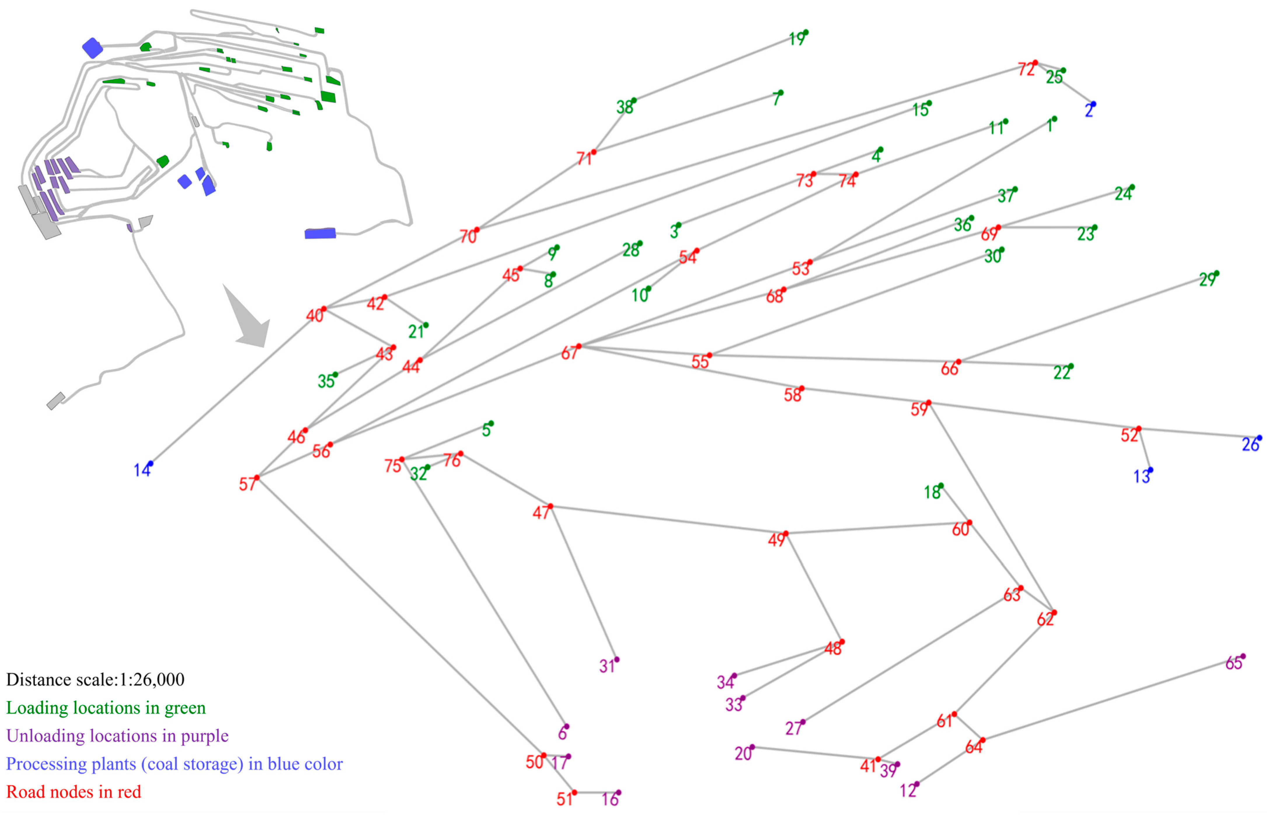
4.2.3. Haulage Routes

This section conducts a comparative analysis between the routes obtained through the traditional staged optimization approach and the integrated optimization approach.

In both scenarios, there are a total of 39 haulage routes utilizing 57 road segments, resulting in a road network utilization rate of 76.0% (i.e., the ratio of the number of utilized road segments to the total number of road segments). However, as shown in Table 7, the traditional approach based on shortest path allocation leads to segments exceeding road capacity limits. In practical operations, operating companies may consider road widening, new road construction, or manual scheduling on-site to circumvent such situations, incurring additional construction or labour costs.

The integrated optimization approach in this study offers two adjustment strategies to comply with road capacity limits. The first strategy is to adjust the mining volume in the production scheduling plan, as illustrated in Figure 12. This disperses the haulage volume across the time dimension. The second strategy is to adjust the unloading locations corresponding to the loading locations, thereby altering the haulage routes. For example, loading location 5, originally paired with unloading location 6, is now paired with unloading location 27. Similarly, loading location 36, initially paired with unloading locations 13 and 17, is now paired with unloading locations 12 and 14, as shown in Figure 13. This disperses the haulage volume across the spatial dimensions.

Therefore, considering road capacity in the integrated optimization of production scheduling and haulage route planning can fully leverage the open-pit mine road network, utilizing existing road capacity and minimizing the need for new road construction.

5. Conclusions

The expenditure generated during production scheduling and transportation is a critical component of the cost structure in open-pit mining. However, the current staged optimization approach is insufficient for devising an effective global mining and haulage plan. Furthermore, planning haulage routes based on predetermined production schedules can lead to road congestion, resulting in additional expenses for road expansion, reconstruction, and manual scheduling. Therefore, there is a need for the integrated optimization of production scheduling and haulage route planning.

To achieve this integration in open-pit mines, our study introduces a two-stage algorithm for determining the mining sequence of large-scale blocks. This approach reduces the computational complexity of the model and establishes spatiotemporal relationships for block mining. Following this, a bilevel optimization model is proposed. The upper-level model focuses on production scheduling optimization, addressing questions such as when and where to mine, how much to mine, and where to send the extracted ore. The lower-level model optimizes haulage routes while considering road capacity using a multi-commodity flow approach. These two models form a feedback mechanism through haulage distance feedback. To solve the model, a solution algorithm with a haulage distance penalty is designed.

The case study results demonstrate that our integrated optimization approach effectively reduces total haulage costs by 10.06%. Therefore, it is necessary for open-pit mines to consider the inter-relationship between production scheduling and transportation planning to effectively reduce transportation costs. The haulage distance feedback mechanism successfully establishes a link between production scheduling and haulage route planning during the model-solving process. Through 42 iterations of distance penalty feedback, the bilevel model is successfully resolved. This feedback mechanism can provide insights for open-pit mine managers to establish the relationship between production scheduling and transportation planning. Additionally, the approach proposed in this study allows for adjusting open-pit mine haulage demand in both temporal dimensions (by modifying monthly mining volumes) and spatial dimensions (through route modifications), effectively preventing road congestion. In the case study, three routes are successfully altered, preventing congestion in five road segments. This indicates that open-pit mine transportation indeed needs to consider the impact of road capacity, which effectively enhances transportation efficiency. Therefore, the integrated optimization approach of production scheduling and haulage route planning proposed in this study facilitates the scientific and rational mining of open-pit mines, offering a viable strategy for cost reduction in open-pit mining.

In future research, integrated optimization models could be enhanced by integrating ore price fluctuations, exploring the effects of dynamic road networks, and incorporating energy constraints for electric mining trucks in haulage route planning.

References

1. Espinoza, D.; Goycoolea, M.; Moreno, E.; Newman, A. MineLib: A Library of Open Pit Mining Problems. Ann. Oper. Res. 2013, 206, 93–114. [Google Scholar] [CrossRef]
2. Das, R.; Topal, E.; Mardaneh, E. A Review of Open Pit Mine and Waste Dump Schedule Planning. Resour. Policy 2023, 85, 104064. [Google Scholar] [CrossRef]
3. Chicoisne, R.; Espinoza, D.; Goycoolea, M.; Moreno, E.; Rubio, E. A New Algorithm for the Open-Pit Mine Production Scheduling Problem. Oper. Res. 2012, 60, 517–528. [Google Scholar] [CrossRef]
4. Xu, X.; Gu, X.; Wang, Q.; Zhao, Y.; Kong, W.; Zhu, Z.; Wang, F. Enumeration Optimization of Open Pit Production Scheduling Based on Mobile Capacity Search Domain. Sci. Rep. 2023, 13, 91. [Google Scholar] [CrossRef]
5. Tabesh, M.; Moradi Afrapoli, A.; Askari-Nasab, H. A Two-Stage Simultaneous Optimization of NPV and Throughput in Production Planning of Open Pit Mines. Resour. Policy 2023, 80, 103167. [Google Scholar] [CrossRef]
6. Elsayed, S.; Sarker, R.; Essam, D.; Coello Coello, C.A. Evolutionary Approach for Large-Scale Mine Scheduling. Inf. Sci. 2020, 523, 77–90. [Google Scholar] [CrossRef]
7. Fu, Z.; Asad, M.W.A.; Topal, E. A New Model for Open-Pit Production and Waste-Dump Scheduling. Eng. Optim. 2019, 51, 718–732. [Google Scholar] [CrossRef]
8. Ma, X.; Zhong, H.; Li, Y.; Ma, J.; Cui, Z.; Wang, Y. Forecasting Transportation Network Speed Using Deep Capsule Networks With Nested LSTM Models. IEEE Trans. Intell. Transp. Syst. 2021, 22, 4813–4824. [Google Scholar] [CrossRef]
9. Yan, H.; Ma, X.; Pu, Z. Learning Dynamic and Hierarchical Traffic Spatiotemporal Features With Transformer. IEEE Trans. Intell. Transp. Syst. 2022, 23, 22386–22399. [Google Scholar] [CrossRef]
10. Liu, X.; Cathy Liu, X.; Liu, Z.; Shi, R.; Ma, X. A Solar-Powered Bus Charging Infrastructure Location Problem under Charging Service Degradation. Transp. Res. D Transp. Environ. 2023, 119, 103770. [Google Scholar] [CrossRef]
11. Bakhtavar, E.; Mahmoudi, H. Development of a Scenario-Based Robust Model for the Optimal Truck-Shovel Allocation in Open-Pit Mining. Comput. Oper. Res. 2020, 115, 104539. [Google Scholar] [CrossRef]
12. Zhang, L.; Shan, W.; Zhou, B.; Yu, B. A Dynamic Dispatching Problem for Autonomous Mine Trucks in Open-Pit Mines Considering Endogenous Congestion. Transp. Res. Part. C Emerg. Technol. 2023, 150, 104080. [Google Scholar] [CrossRef]
13. Zhang, X.; Guo, A.; Ai, Y.; Tian, B.; Chen, L. Real-Time Scheduling of Autonomous Mining Trucks via Flow Allocation-Accelerated Tabu Search. IEEE Trans. Intell. Veh. 2022, 7, 466–479. [Google Scholar] [CrossRef]
14. Liu, X.; Qu, X.; Ma, X. Optimizing Electric Bus Charging Infrastructure Considering Power Matching and Seasonality. Transp. Res. D Transp. Environ. 2021, 100, 103057. [Google Scholar] [CrossRef]
15. Samavati, M.; Essam, D.; Nehring, M.; Sarker, R. A Local Branching Heuristic for the Open Pit Mine Production Scheduling Problem. Eur. J. Oper. Res. 2017, 257, 261–271. [Google Scholar] [CrossRef]
16. Moreno, E.; Rezakhah, M.; Newman, A.; Ferreira, F. Linear Models for Stockpiling in Open-Pit Mine Production Scheduling Problems. Eur. J. Oper. Res. 2017, 260, 212–221. [Google Scholar] [CrossRef]
17. Epstein, R.; Goic, M.; Weintraub, A.; Catalán, J.; Santibáñez, P.; Urrutia, R.; Cancino, R.; Gaete, S.; Aguayo, A.; Caro, F. Optimizing Long-Term Production Plans in Underground and Open-Pit Copper Mines. Oper. Res. 2012, 60, 4–17. [Google Scholar] [CrossRef]
18. Jélvez, E.; Morales, N.; Nancel-Penard, P.; Peypouquet, J.; Reyes, P. Aggregation Heuristic for the Open-Pit Block Scheduling Problem. Eur. J. Oper. Res. 2016, 249, 1169–1177. [Google Scholar] [CrossRef]
19. Boland, N.; Dumitrescu, I.; Froyland, G.; Gleixner, A.M. LP-Based Disaggregation Approaches to Solving the Open Pit Mining Production Scheduling Problem with Block Processing Selectivity. Comput. Oper. Res. 2009, 36, 1064–1089. [Google Scholar] [CrossRef]
20. Alipour, A.; Khodaiari, A.A.; Jafari, A.; Tavakkoli-Moghaddam, R. An Integrated Approach to Open-Pit Mines Production Scheduling. Resour. Policy 2022, 75, 102459. [Google Scholar] [CrossRef]
21. Paithankar, A.; Chatterjee, S. Open Pit Mine Production Schedule Optimization Using a Hybrid of Maximum-Flow and Genetic Algorithms. Appl. Soft Comput. J. 2019, 81, 105507. [Google Scholar] [CrossRef]
22. Gilani, S.O.; Sattarvand, J.; Hajihassani, M.; Abdullah, S.S. A Stochastic Particle Swarm Based Model for Long Term Production Planning of Open Pit Mines Considering the Geological Uncertainty. Resour. Policy 2020, 68, 101738. [Google Scholar] [CrossRef]
23. Choi, Y.; Park, H.D.; Sunwoo, C.; Clarke, K.C. Multi-Criteria Evaluation and Least-Cost Path Analysis for Optimal Haulage Routing of Dump Trucks in Large Scale Open-Pit Mines. Int. J. Geogr. Inf. Sci. 2009, 23, 1541–1567. [Google Scholar] [CrossRef]
24. Choi, Y.; Nieto, A. Optimal Haulage Routing of Off-Road Dump Trucks in Construction and Mining Sites Using Google Earth and a Modified Least-Cost Path Algorithm. Autom. Constr. 2011, 20, 982–997. [Google Scholar] [CrossRef]
25. Li, X.; Gu, Q.; Ruan, S.; Feng, Z. Optimal Transportation Path Planning of Truck in Open-Pit Mine under Dynamic Energy Consumption. J. China Coal Soc. 2021, 46, 590–600. [Google Scholar] [CrossRef]
26. Ramazan, S. The New Fundamental Tree Algorithm for Production Scheduling of Open Pit Mines. Eur. J. Oper. Res. 2006, 177, 1153–1166. [Google Scholar] [CrossRef]
27. Lang, A.; Schubert, E. BETULA: Fast Clustering of Large Data with Improved BIRCH CF-Trees. Inf. Syst. 2022, 108, 101918. [Google Scholar] [CrossRef]
28. Lorbeer, B.; Kosareva, A.; Deva, B.; Softić, D.; Ruppel, P.; Küpper, A. Variations on the Clustering Algorithm BIRCH. Big Data Res. 2018, 11, 44–53. [Google Scholar] [CrossRef]
29. Zhou, J.; Love, P.E.D.; Teo, K.L.; Luo, H. An Exact Penalty Function Method for Optimising QAP Formulation in Facility Layout Problem. Int. J. Prod. Res. 2017, 55, 2913–2929. [Google Scholar] [CrossRef]
30. Wang, Y.; Assogba, K.; Fan, J.; Xu, M.; Liu, Y.; Wang, H. Multi-Depot Green Vehicle Routing Problem with Shared Transportation Resource: Integration of Time-Dependent Speed and Piecewise Penalty Cost. J. Clean. Prod. 2019, 232, 12–29. [Google Scholar] [CrossRef]
31. Liu, X.; Liu, X.; Zhang, X.; Zhou, Y.; Chen, J.; Ma, X. Optimal Location Planning of Electric Bus Charging Stations with Integrated Photovoltaic and Energy Storage System. Comput.-Aided Civil. Infrastruct. Eng. 2023, 38, 1424–1446. [Google Scholar] [CrossRef]
32. Zhang, T.; Ramakrishnan, R.; Livny, M. BIRCH: A New Data Clustering Algorithm and Its Applications; Kluwer Academic Publishers: Dordrecht, The Netherlands, 1997; Volume 1. [Google Scholar]
33. Das, R.; Topal, E.; Mardaneh, E. Concurrent Optimisation of Open Pit Ore and Waste Movement with Optimal Haul Road Selection. Resour. Policy 2024, 91, 104834. [Google Scholar] [CrossRef]
34. Sun, X.; Zhao, S.; Liu, H.; Zhang, H. Equilibrium Distribution Model of Traffic Flow on Road Network for Traffic Flow of Open Pit. J. China Coal Soc. 2017, 42, 1607–1613. [Google Scholar] [CrossRef]
35. Wang, J.; Zhao, N.; Xiang, L.; Wang, C. Abnormal Cascading Dynamics Based on the Perspective of Road Impedance. Phys. A Stat. Mech. Its Appl. 2023, 627, 129128. [Google Scholar] [CrossRef]
36. Chen, J.; Mei, Z.; Wang, W. Road Resistance Model under Mixed Traffic Flow Conditions with Curb Parking. China Civil. Eng. J. 2009, 40, 95–100. [Google Scholar]
Figure 1. Open-pit mine production and transportation process.
Mathematics 12 02070 g001
Figure 2. Research framework.
Mathematics 12 02070 g002
Figure 3. Algorithm flowchart for determining the mining sequence of blocks.
Mathematics 12 02070 g003
Figure 4. Mining sequence illustration of clusters.
Mathematics 12 02070 g004
Figure 5. Algorithm solution flowchart.
Mathematics 12 02070 g005
Figure 6. Distribution map of clusters.
Mathematics 12 02070 g006
Figure 7. Schematic diagram of the open-pit mine road network.
Mathematics 12 02070 g007
Figure 8. Iterative plot of the total objective value.
Mathematics 12 02070 g008
Figure 9. Monthly haulage volume at the loading and unloading locations.
Mathematics 12 02070 g009
Figure 10. Schematic diagram of the relationship between road transit time and haulage volume.
Mathematics 12 02070 g010
Figure 11. Model solving process.
Mathematics 12 02070 g011
Figure 12. Monthly haulage volume.
Mathematics 12 02070 g012
Figure 13. Route comparison.
Mathematics 12 02070 g013