Abstract
This study introduces a novel approach to data gathering in energy-harvesting wireless sensor networks (EH-WSNs) utilizing cooperative multi-agent reinforcement learning (MARL). In addressing the challenges of efficient data collection in resource-constrained WSNs, we propose and examine a decentralized, autonomous communication framework where sensors function as individual agents. These agents employ an extended version of the Q-learning algorithm, tailored for a multi-agent setting, enabling independent learning and adaptation of their data transmission strategies. We introduce therein a specialized -p-greedy exploration method which is well suited for MAS settings. The key objective of our approach is the maximization of report flow, aligning with specific applicative goals for these networks. Our model operates under varying energy constraints and dynamic environments, with each sensor making decisions based on interactions within the network, devoid of explicit inter-sensor communication. The focus is on optimizing the frequency and efficiency of data report delivery to a central collection point, taking into account the unique attributes of each sensor. Notably, our findings present a surprising result: despite the known challenges of Q-learning in MARL, such as non-stationarity and the lack of guaranteed convergence to optimality due to multi-agent related pathologies, the cooperative nature of the MARL protocol in our study obtains high network performance. We present simulations and analyze key aspects contributing to coordination in various scenarios. A noteworthy feature of our system is its perpetual learning capability, which fosters network adaptiveness in response to changes such as sensor malfunctions or new sensor integrations. This dynamic adaptability ensures sustained and effective resource utilization, even as network conditions evolve. Our research lays grounds for learning-based WSNs and offers vital insights into the application of MARL in real-world EH-WSN scenarios, underscoring its effectiveness in navigating the intricate challenges of large-scale, resource-limited sensor networks.
Keywords:
reinforcement learning; Q-learning; wireless communication; wireless sensor network; data-gathering; multi-agent systems; cooperative systems; autonomous communication; distributed algorithms; medium-access control protocols; energy harvesting MSC:
90C40; 93E35
1. Introduction
In the era where the dynamics of big data shape the trajectory of technological advancements, the significance of wireless sensor networks (WSNs) in various applications has become paramount. These networks, integral to fields as diverse as environmental monitoring, health care, industrial automation, and urban infrastructure management, are linchpins in the modern data-driven decision-making landscape. WSNs stand at the forefront of capturing, processing, and transmitting invaluable real-time data, crucial for timely and informed decisions across multiple sectors. Characterized by a diverse array of sensor capabilities and operating under various constraints such as limited energy, bandwidth, and computational power, WSNs face formidable challenges in the efficient and effective gathering of data. Traditional methodologies for data collection in these networks, though tailored to specific network types and demands, are increasingly seen as insufficient for addressing the complexity of sensor constraints. Characterized by substantial coordination overhead and a lack of adaptability to changing environmental and operational conditions, these methods have shown limitations in terms of scalability and flexibility to different constraints. This has led to burgeoning interest in developing more dynamic, intelligent, and efficient data-gathering strategies, fueled by the rapid advancements in the fields of artificial intelligence and machine learning. These technologies, with their immense potential, are poised to revolutionize the operational paradigms of WSNs by enhancing their flexibility, adaptability, and overall efficiency.
With the evolution of machine learning (ML), which has become a trend utilized in practically every aspect of our lives, it seems only natural to incorporate such techniques in WSNs and, in particular, data-gathering applications wherein resources such as sensors’ capabilities (e.g., energy, memory) and airtime are limited. Although potentially capable of providing very satisfactory results, the traditional centralized ML approach, and specifically reinforcement learning (RL), in which a centralized decision-maker observes, learns, and controls the sensors’ behavior, seems inappropriate due to the significant overhead involved in collecting and distributing information between the central entity (e.g., access point or sink) and the numerous sensors, as well as the scalability issues and delay incurred for adaptations to real-time changes. Accordingly, a distributed approach seems much more appropriate; distributed RL empowers individual sensors to make independent decisions in response to their immediate environments. This autonomy not only reduces overhead, but is also crucial for networks that require rapid adaptability to constantly changing environmental conditions, fluctuating resource availability, and evolving network dynamics. However, the generalization of the single decision-maker RL to a multi-agent framework presents a myriad of challenges. Foremost among these is the issue of non-stationarity in network environments and the intricacies involved in achieving optimal strategic convergence among a multitude of simultaneously interacting sensors.
Our research endeavors to investigate both the potential and the complexities involved in adopting a multi-agent reinforcement learning (MARL) approach in the context of WSNs. Specifically, we explore various MARL mechanisms and their implications for sensor network dynamics, as well as the reciprocal impact of sensor network dynamics on MARL. Our aim is to understand key contributing factors and identify mechanisms for achieving high-performing, adaptively learning wireless networks. This work provides insights as a stepping stone for future research and demonstrates the potential of an MARL-based approach for optimized data-gathering in WSNs.
To explore the applicability of MARL to WSNs, we employ a pervasive data-gathering use case in which multiple sensors must report an observed phenomenon to a sink (or a set of sinks). The specific sensor that reports the observation is irrelevant as long as the sink receives continuous reports. We assume that the sensors are constrained by energy, which they need to harvest from the environment, i.e., a sensor can transmit a report only after it has harvested sufficient energy for such transmission. We assume that each sensor executes a Q-Learning algorithm with a limited state space. It is important to emphasize that the Q-Learning algorithm executed by the various sensors is completely distributed, meaning that the sensors do not exchange any information between them and do not include any additional information in their reports other than what is required by the protocol used. Although there are more advanced mechanisms, such as deep RL, which can handle large systems and provide superior results, we adopted Q-learning for two main reasons. First, we believe the sensors have limited capabilities and resources, which constrain them from running more complex mechanisms. Second, and more importantly, since the aim of this paper is to explore the potential of employing MARL for data-gathering in WSNs, we believe that utilizing Q-learning can provide better insight into the dynamics of the system.
By exploring the Q-table obtained and the strategies adopted by various sensors for various setups, we gained insights into some important factors that affect whether the system will converge to high network utilization (a continuous stream of reports received by the sink) or to a poor one. We demonstrate that under mild conditions, the system can converge to optimal performance, where the sensors learn to transmit in a time division multiple access (TDMA)-like pattern by learning to avoid synchronization. For dense networks, we observe high airtime utilization, yet suboptimal performance, as some sensors learn to avoid transmission altogether while others transmit. To incentivize sensors to remain idle in case of collisions, we devised a global reward for successful transmission attained by all sensors, regardless of the transmitting sensors. Additionally, we leveraged insights from the backoff mechanism in random access protocols, biasing the action to remain idle on transmit while in exploration mode. This allowed each sensor to explore transmission only once in every several visits to the exploration mode.
The distinctiveness of our work is manifold. Primarily, it facilitates the autonomous adaptation of transmission strategies by sensors, based on indirect real-time assessments of channel usage. Moreover, our approach is completely distributed and makes use of no coordination overhead, which is related to the learning process, i.e., no extra over-the-air control overhead other than what is required by the channel access protocol, e.g., communication headers, acknowledgments, etc. Avoiding such communication overhead is paramount to ensure that the network can effectively fulfill its data-reporting objectives, utilizing the airtime by transmitting reports rather than wasting the majority of the airtime by transmitting learning information, as suggested by several other studies aiming to obtain a superior strategy.
This study focuses on learning deterministic policies in discrete environments and available actions, delving into the fundamental understanding of cooperative system dynamics. We demonstrate high efficiency in various homogeneous and heterogeneous scenarios by applying networking concepts that assist sensors in obtaining medium access coordination. Emphasizing its suitability for small and simple hardware devices, our distributed approach maintains minimal memory and computing power usage and does not require centralized training. With a continuous learning algorithm approach, we demonstrate adaptability to changing network dynamics, which is crucial for maintaining the flow of sensor reports. Combining these valuable conceptual elements, we present an implementation of our proposal, discussing its applicability and practicality in the real world. Highlighting our findings and emphasizing the broad implications of our research, we designate this research as facilitating the evolution and understanding of autonomous learning data gathering in WSNs.
To summarize, the contribution of our research is as follows:
- We provide a simple multi-agent energy-harvesting wireless sensor network (EH-WSN) model for data gathering, where the objective is for the sink to receive as many reports as possible, regardless of the identity of the senders. The system relies on global rewards received by all sensors whenever an ACK is transmitted by the sink, incentivizing the sensors to collaborate rather than contend. The suggested procedure is completely distributed and free from control messaging or any information exchange.
- The model adapts the single-agent Q-Learning algorithm to a multi-agent Q-Learning algorithm, which is suited for simple hardware, where each sensor runs the Q-Learning algorithm distributively. The results show up to 100% channel utilization, where sensors learn to transmit in a TDMA-like pattern.
- To address WSNs with a large number of sensors, we introduce a specialized version of the -greedy policy, termed -p. This policy provides a novel networking-inspired exploration mechanism that is well suited for Q-learning within a multi-agent system environment, particularly when the number of agents is large.
- We address challenging scenarios where sensors have differentiated EH patterns. To do so, we augment the model by expanding the state-space with additional parameters, which also require no control or inter-sensor information exchange. In this setup, the sensors demonstrate a transmission pattern that achieves very high (sometimes up to 100%) channel utilization. The system is shown to be robust to topological changes, such as adapting to a sensor’s failure and a new sensor joining the WSN.
- The results are thoroughly analyzed, and various parameters and settings are explored. We provide insight into many issues that can be leveraged for other setups and scenarios.
- We provide a hardware implementation that clearly validates the findings using a software-defined radio. The real-time implementation demonstrates that the procedure can operate and attain similar satisfactory results to those achieved in simulation, over a physical medium, despite additional challenges such as fading, noise, ACK de-synchronization, and others.
This paper aims to shed light on the potential of using MARL for the prevalent application of data gathering in WSNs, covering crucial aspects. It is organized as follows: Section 2 reviews the related literature on reinforcement learning in the context of WSN data gathering and medium access control. Section 3 provides basic background on reinforcement learning and multi-agent systems, setting the stage for our subsequent discussions. Section 4 introduces the model used throughout the paper. Section 5 unfolds our RL design, and Section 6 presents the MARL algorithm, elucidating the intricate mechanisms underpinning our approach’s advancements in sensor network efficiency and performance. Section 7 presents simulation results covering a diverse range of setups accompanied by a thorough analysis of the results. Section 8 bridges the gap between theory and practice, presenting an implementation of the suggested algorithm using a software-defined radio (SDR). Finally, Section 9 concludes the paper.
2. Related Work
Gathering data in wireless sensor networks has been a prolific research topic over the last few decades, with a myriad of optimizing proposals developed across all layers of the OSI model [1]. Wireless sensor networks architecture can be typically divided into two types according to the overall objectives: network-based, where the network’s topology dictates algorithmic considerations (e.g., coverage, aggregation, latency), and sensor-characteristics-based, where the sensor may be constrained in the ability to transmit freely (e.g., energy harvesting, battery). Typically, in some of those cases, data-gathering is application-oriented, where the eventual need for reports follows to satisfy a specific demand by the application. While the aim is to satisfy all demands and constraints, in most cases, genericness is not possible, and the proposed works focus on satisfying specific objectives. Over the years, several protocols have been proposed to meet different applicative requirements. One of the earliest, and perhaps most prominent, was the ALOHA protocol [2], a simple random access protocol, where each user can transmit data whenever it has packets to send, and collisions may occur when multiple users transmit simultaneously, incurring a basic retransmission mechanism. It is well known that in such an ill-informed approach, medium utilization and performance must be sacrificed. To address such challenges and others, numerous advanced protocols have been proposed over the last few decades. Many of those protocols have been surveyed extensively in [1,3,4]. Each of the protocols was designed with various considerations, such as energy [5,6], network dynamics, throughput and utilization [7], fault recovery [8], latency [9], and more. These proposals cater to a multitude of different application needs and aim to address them efficiently [10]. When concerning controlling access to the transmission medium, there are numerous methods in use, from duty-cycling transmission times [11] to listening and sleeping times, either synchronously [12] or asynchronously [13] among participating sensors, locality-based clustering of WSN into hierarchical groups to perform a congestion control [14], as well as certain heuristics approaches like the receiver-initiated paradigm [15]. In many cases, trade-off considerations come into play throughout all design aspects. For example, energy–timing considerations [16], waiting to save energy expenses, or quickly delivering to a sink [17,18]. Traditionally, such non-learning-based protocols were strict, assigning channel resources to network parties in either static or dynamic mode, where each sensor is given a periodic interval where it can perform transmission uninterruptedly. On the other hand, certain works enabled the use of probabilistic approaches, usually associated with learning, that necessitated the adjustment of parameters for optimal performance. Recent research [19] introduces communication-efficient workload balancing for MARL, suggesting that workload be balanced among agents through a decentralized approach, allowing slower agents to offload part of their workload to faster agents. This minimizes the overall training time by efficiently utilizing available resources. While the proposed solution clearly implies an additional (even though distributed) communication overhead, it may be deployed in parallel to the learning model, such as ours. Over the days, medium-access studies have made a tremendous leap toward improvement in many of the above domains, yet perhaps the biggest leap came with the rise of learning techniques [20]. In the following, we present a literature review of approaches to data gathering in wireless sensor networks. We mainly place our focus on learning-based medium access control [21], particularly those who use real-time reinforcement learning methods [22]. This review is divided into two subsections: The first reviews recent machine learning (ML) and reinforcement learning (RL) approaches. The second part of the review incorporates more detail, examining state-of-the-art research that focuses on multi-agent reinforcement learning approaches.
2.1. Reinforcement Learning Approaches
In recent times, with the advancement of computational technology and learning techniques, new artificial intelligence (AI) and machine learning (ML) approaches came to exist [23], where sensors and sinks model and learn a behavioral scheme most suitable for their objectives [22]. The idea that WSN’s behavior can be defined in software [24] makes it multi-functional and more flexible, more suited to the applications at hand. The use of ML/AI in wireless sensor networks takes many forms of implementation techniques [25,26]. These techniques have huge potential for improving and optimizing various paradigms in WSNs. The recent integration trends of such tools facilitated the rapid advancement of technology [27], leading to new research directions. Particularly, it has opened up a variety of new possibilities for optimizing data collection and management in WSNs, leading to improved network performance, energy efficiency [28], QoS [29], and overall system reliability [30], whereas for the wireless medium, such novelties vary from the physical layer, where transmission settings are set (e.g., transmission power [31], modulation and coding schemes [32], network coding [33], channel modeling [34,35], etc.) through the data link layer (e.g., medium access control [22,36], link control [37], scheduling [38], etc.) and up to the network layer (e.g., routing [39], spanning and clustering [40], etc.). Computationally, the recent quantum multi-agent reinforcement learning for aerial ad hoc networks was proposed in [41], specifically focusing on the use of quantum computing employed for RL (particularly, multi-agent proximal policy optimization) to improve the connectivity of flying ad hoc networks. Nevertheless, designing ML/AI MAC protocols comes with a merit of challenges and limitations [42], which must be carefully addressed.
In controlling access to the transmission medium (MAC) in WSNs, the majority of works utilize a reference model of an MAC protocol, optimizing essential aspects by learning the optimal tuning parameters [22]. Using ML to classify and identify MAC protocols, ref. [43] can be utilized for applying the appropriate RL approach to learn and optimize medium access at hand [44]. By solving an MDP model, ref. [45] learned the optimal back-off schemes in systems with unknown dynamics. An example work that uses a model as a reference is UW-ALOHA-QM [46], a fully distributed RL-based MAC protocol that builds on and improves the popular ALOHA random access approach. It [46] was designed with the goal of efficiently managing the transmission of data packets in a challenging underwater environment. The authors of [46] proposed learning the discretized sensor’s best sub-frame access timings according to the propagation delays of each sensor with respect to a sink. The work in [47] proposed DR-ALOHA-Q, an asynchronous learning method for transmission-offset selection, which also uses ALOHA as a reference. The possible selection of sub-frame time is pre-defined as the possible actions a sensor decides upon. In addition, in [47], sensors may dynamically change their decision as sensors move and the respective delay changes. Different learning techniques are applied to optimize different traditional transmission schemes, such as time division [48], or as in the aforementioned ALOHA. In QL-MAC [49], an optimization of CSMA was proposed, using a Q-Learning-based MAC protocol that aims to adapt the sleep–wake-up duty cycle while learning other nodes’ sleep–wake-up times. Synonymously, the CSMA proposed in [50] optimizes the contention probability, dynamically tuning it by RL. The work in [51] proposed a data aggregation scheduling policy for WSNs using Q-Learning. A cognitive radio spectrum sensing–transmission framework for energy-constrained WSNs using actor–critic learning was presented in [52]. Model-based works are eventually limited by the theoretical performance bounds of that particular model it strives to optimize. Opposed to basing on those traditional modeled schemes and approaches, a DLMA [53] sensor assumes that other users on the common time-slotted medium make use of some general MAC protocol, as it operates to learn an optimal channel access policy of its own corresponding to other participants’ access policy.The authors of [54] presented LEASCH, a deep reinforcement learning (DRL) model able to solve the radio resource scheduling problem in the MAC layer of 5G networks, replacing the standards’ radio resource management (RRM). Based on online learning [55], Learn2MAC [56] proposes a protocol for uncoordinated medium access of IoT transmitters competing for uplink resources. In the following subsection, this model-free principle is further discussed as multi-agent networks allow for a higher level of sensor decision autonomy.
Recent Results on Q-Learning Convergence
As we shall further present, the algorithm being run by every sensor is our custom flavor of Q-Learning (QL). Since there are several novel results regarding the convergence bound, we shortly mention some of those and remark on a possible relation to the system model presented in this work. We firstly focus on the most recent [57], which sharpens convergence bounds for QL providing tighter bounds. Note that only results on the asynchronous QL are relevant to our work. This is because we research a real-time system and the Q-value for only one pair of state–action can be updated at each sample (i.e., time slot). For the asynchronous case, the authors in [57] provided bounds of Q-values convergence accuracy within some given distance from the theoretical optimum (i.e., the Bellman equation fixed point). These bounds are demonstrated to be sharp for the ordinary, i.e., the single-agent setting. Hence, the application of such bounds to our model would be problematic because the problem of convergence in a multi-agent setting is not sufficiently understood and remains essentially open. An additional assumption is made therein, including dependence on the length of the sample path (the number of transmission time slots that each sensor would learn in total), knowledge of the minimum state–action occupancy probability, and having a constant learning rate depending on the length of the sample path. These assumptions do not agree with the way the parameters are particularly tailored in our experiments (see the section that follows). More results from recent years along with older results are presented in a table within this work. Additional recent research of asynchronous QL appears in [58]. This work provides a bound expressed by two components; there, the first component matches a result that bounds the error by similar yet in the synchronous case, and the second component expresses the probabilistic properties of the sample path through the mixing time (is derived using minimum state–action occupancy probability; see the precise definitions therein). We note that comparison with our experiments would experience the same difficulties as mentioned.
We finally mention the earlier ground-laying work in [59] also providing bounds for asynchronous QL, but a polynomial decrease in the learning rate is assumed. Moreover, the expression therein depends on knowledge of the covering time which relates to the number of samples before visiting all possible state–action pairs. Their results are long experimentally proven; however, the polynomial rates cannot be applied to our system.
Henceforth, we stress the experimental nature of our work; therefore, we opt to delay the theoretical analysis of convergence bounds to future work.
2.2. Multi-Agent Reinforcement Learning Approaches
Many of the reinforcement learning approaches assume the perspective of a single agent, as it stands alone in its optimization task, while in a network where multiple learners act simultaneously, known as a multi-agent system (MAS) [60], the operative perspective changes to accommodate the resulting dynamics among agents [61]. Commonly, multi-agent system paradigms mainly tend to coordinate [62] and control [63] problems. Applying an RL-MAS perspective to the data-gathering task in WSNs allows a high degree of sensor autonomy where agents collectively perform various objective optimizations as independent decision-makers as well as a collective. In [64], the authors proposed deep Q-Learning (QL) centralized training and distributed execution (CTDE) for spectrum sharing with cooperative rewards. In [65], a CTDE multi-agent deep deterministic policy gradient (MADDPG) algorithm was used. Ref. [66] proposed a CTDE MAC protocol with fairness and throughput considerations. Some propose a different approach, where agents must learn new communication protocols in order to share information that is needed to solve tasks. The work in [67], named Learning to communicate, used reinforced inter-agent learning (RIAL) and differentiable inter-agent learning (DIAL), architecture as a CTDE multi-agent network. Ref. [65] presented a broader approach to MAC protocols, dropping many of the common rules and enabling a base station and the user equipment to come up with their own medium access control. With a goal of learning to generalize MAC, the work in [68] used multi-agent proximal policy optimization (MAPPO) along with autoencoders and was based on observation abstraction to learn a communication policy in which an MAC protocol caters to extremely diverse services across agents requiring different quality of service. The recent work of [69] studied agents deployed over UAVs (comparatively large, hence storage and computation-wise capable units), where the agent’s state-space includes precise data about all other agents. This is contrary to our setting. As a novelty, the authors incorporated an attention mechanism at every agent. It is clear that such a computational effort cannot be attained in tiny information-collecting sensors.
CTDE as an MARL architecture is based on transferring the insight learned from the centralized entity, a sink, or a base station across all agents, which comes at the cost of overhead information. The topological nature of data-collecting networks, having a sink that siphons the data reports, does not oblige the learning to be centralized. Although CTDE is a very popular MARL framework, some claim that it is not enough for MARL [70] and agents should make their own decisions only based on decentralized local policies. The research in [71] aimed to address challenges in learning methodology and efficient sampling (during the learning process). Policy explainability in MARL was explored. Some of the explored techniques, identification of high-rewarding state–action pairs, and assigning positive rewards to specific joint state–action pairs that, during the learning process, subsequently lead to valuable pairs within the trajectory are highlighted. A multi-agent approach where each sensor acts autonomously may alleviate the need for interchanging learning parameters and insight overhead across the networks. Contrary to those centralized learning approaches, decentralizing the learning, as in [72], where cooperative MARL deep Q-Learning was used for dynamic spectrum access, may come as an advantage in terms of the overhead required for obtaining proper coordination. Similarly, schedule-based cooperative MARL for multi-channel communication in wireless sensor networks was proposed in [73]. The cooperation among agents is facilitated through the use of a shared schedule, which coordinates their actions and ensures efficient channel utilization. For example, in [74], partial information was shared among agents. In such approaches, agents communicate with each other to exchange information about their observations and learning policies, enabling them to make more informed decisions, but at the cost of overhead in the form of inter-sensor communication. Designing a cooperative reward that would be particularly tailored for a system objective remains an insufficiently explored area. This is because the topic is heuristic, depends on a specific scenario, and lacks any known mathematical framework. A recent attempt to address reward design for MARL is seen in [75]. This system, however, accounts for asymmetric agents while addressing both global and agent-specific goals in simulations. Such a goal design can only be exploited in scenarios of interest and cannot be generalized.
In the work proposed in [76], the IEEE 802.15.4 Time-Slotted Channel Hopping (TSCH) schedule was optimized with a contention-based multi-agent RL approach. The best time slot and channel hopping pattern are learned from the predefined resource block structure available. Providing network sensors with full autonomy to make decisions based only on their own perspective has the advantage of alleviating most of the overhead.
Evaluation of scaling MARL to explore a high number of agents is an ongoing research area being conducted nowadays; see one of the most recent in, e.g., [77]. Furthermore, large-scale networks are too complex for a single centralized entity to manage the extremely high number of possible joint states and actions of all sensors. Therefore, such a distributed multi-agent learning approach is considered more plausible.
In [78], the network is dynamic, with sensors entering and leaving the network at random. Furthermore, throughput and fairness guarantees are provided among participating sensors at all times. Despite successful applications of multi-agent systems [79], particularly to wireless networks, simultaneous autonomous learning converging to optimal performance is deemed somewhat problematic in some systems. This is a result of some well-known multi-agent pathologies [80] that pose an issue to solving many paradigms, which need to be addressed accordingly. To mention one of the most recent attempts to understand the related difficulties, we note a multi-agent optimistic soft QL introduced in [81]. The main idea is to first calculate the local Q-function using the global Q-function, and then determining the local policy based on that local Q-function. This method is termed as a projection of the global Q-function onto local Q-function. Nevertheless, MARL, with its immense potential is a promising avenue for future research on the wireless medium, particularly in data-gathering WSNs.
3. Reinforcement Learning Preliminaries
In the following, we provide a basic background on reinforcement learning, with a focus primarily on reinforcement learning within multi-agent systems. Readers who are familiar with the topic may skip this fundamental overview.
3.1. Q-Learning
Reinforcement learning (RL) is a type of machine learning technique that enables an agent to learn in an interactive environment by trial and error using feedback from its own actions and experiences in order to maximize the notion of cumulative reward.
An agent is supposed to decide the best action a to take based on his current state s. It decides that either based on some model of the environment, where it only has to learn the optimal actions to take, achieved by a solution of an MDP, or without a model (model-free) where it iteratively updates its estimates of its expected future return, updating value to taken actions at every state. After taking the action, it transitions to a new state and obtains a reward r. One of the most widely used model-free algorithms is the Q-Learning algorithm [82]. It operates by maximizing expected future returns over successive time steps t, starting from any starting state s. The core of the algorithm is based on estimating the solution to the Bellman equation, expressed as a state–-action quality function (termed Q-value). Iterative updates constitute the weighted average of the previously learned Q-value and new information (see, e.g., [83,84]):
where is a future discount factor, , and is the learning rate which determines to what extent newly acquired information overrides prior learned information. Figure 1 illustrates this iterative cycle which stands as the base of reinforcement learning.

Figure 1.
Basic reinforcement learning.
3.2. Multi-Agent Systems
A system composed of multiple autonomous intelligent entities known as agents is referred to as an MAS [60]. Multi-agent systems are able to deal with learning tasks deemed difficult or impossible for an individual agent. These systems consist of agents and a shared environment in which they act and learn. Each agent decides on and takes action with the aim of solving the task at hand. MAS architecture can take many forms, depending on the specific application domain, the nature of the agents involved, and the goals of the system. A general description of the multi-agent system reinforcement learning is depicted in Figure 2. Agents in the system can be in a cooperative environment setting, competitive, or a combination of both. Their training and execution methods can be centralized or decentralized. Agents can have full or partial information about their neighboring agents (e.g., states, actions, observations, parameters), or none at all. The agents may withhold from sharing information or implicitly communicate with each other, or with a central entity. No agent has a full global view. The system is too complex for an agent to exploit such knowledge.
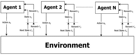
Figure 2.
Basic multi-agent system reinforcement learning.
All agents employ a learning algorithm in which, at a given time, they simultaneously observe the environment and take actions, either independently or jointly, thereby affecting the shared environment. They then receive a reward and transition from their current state to a new state, again, either independently or jointly. Agents can all share the same perspective of the environment, where they all receive the same state information, or they can each have an individual partial view of the environment. Despite the recent success of reinforcement learning and deep reinforcement learning in single-agent environments, there are many challenges when applying single-agent reinforcement learning algorithms to multi-agent systems due to several problems that arise [80]. In the independent learner coordination problem, cooperative independent learners (ILs) must coherently decide on their individual actions such that the resulting joint action of the entire MAS is the best possible. Another issue is the non-stationary problem, which arises because, from the perspective of each agent, the other agents are considered part of the environment. Since the agents’ behavior is changing in accordance with their learning process, from the single-agent perspective, the environment is non-stationary. In addition, the agent view can be affected by noise and other observable factors, causing a stochasticity problem, which can mislead learning. As a core principle, an agent has to balance an exploration–exploitation trade-off which exposes actions made not as a result of a learned policy, but randomly. This alter-exploration problem is considered as random noise from the single-agent view. Action shadowing occurs when one individual action appears better than another, even though the second is potentially superior. This is the result of the fact that agents receive rewards based on the joint action yet keep value for their own individual actions. Consequentially, reaching a coordination equilibrium may not be possible with the agent’s optimal policy, also termed the shadowed equilibrium problem. If any of these problems are present in a naive MAS, it would probably behave poorly (i.e., sub-optimally), failing to reach coordination. For that, one must carefully design the state and action spaces and properly engineer an agent’s reward function.
4. System Model
Wireless sensor networks are commonly deployed to monitor and report various phenomena across areas of interest. Such networks may include numerous sensor units that may have different report capabilities and contributions to the general applicative goal. Typically, sensors are limited by some physical constraints (e.g., available energy, transmission power, sample periodicity, etc.), which constrains their ability to deliver reports to a data-gathering sink. In this section, we describe the system model.
We assume a wireless sensor network that collects reports from the covered area. The network consists of a single sink (access point) that collects the reports from the sensors. The set of sensors is denoted by and denotes the total number of sensors in the network. We assume that each sensor can communicate with the sink node directly (one hop). We consider an application that demands a maximal flow of reports regardless of the identity or location of the reporting sensor, i.e., reports from all sensors have equal value to the application. All reports are similar in length and the sink acknowledges each successful report (sends ACK). Figure 3 illustrates the system model, in which an RL-based Sensor 8 sends a report to the gateway. The gateway successfully receives the report and sends an ACK in return, which is received by all the other RL-based sensors. The time is slotted and the transmission rate of all sensors is fixed such that the slot duration is sufficient to transmit a single report and the corresponding ACK. We assume perfect synchronization between the sensors and the sink (the sink periodically transmits a beacon to synchronize all the sensors). All transmissions start at the beginning of a slot, and we assume an errorless collision model, meaning a single transmission heard at a node is always successful. In contrast, if two or more transmissions overlap in time at the receiver (i.e., there is a collision), they are not received correctly.
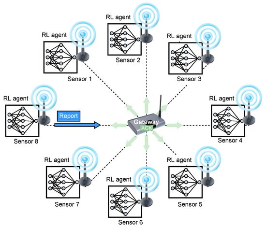
Figure 3.
An illustration of the system model comprises 8 RL-based sensors and a gateway sink. The figure shows an example of a single time slot in which Sensor 8 sends a successful report (no other sensors have sent reports simultaneously). This report is responded to by a broadcasted ACK sent by the gateway, which is received by all other RL-based sensors.
Sensors are limited by energy constraints, allowing them to transmit only when their batteries have enough energy. We assume that the sensors rely on energy harvesting; specifically, each sensor’s energy level depends on the energy it harvests from the environment (e.g., [85]) and its activity (recent transmissions). We assume that the charging rate of sensor is fixed and will be denoted by [energy units per time slot]. The energy a sensor can store is limited and will be denoted by . The energy required to transmit a report is fixed for all sensors and will be denoted by [energy units per transmission]. We assume that energy charging does not occur during transmission. We assume that both the energy required for transmission and the maximal energy a sensor can store is an integer multiple of the energy harvested per slot, i.e., , and . As previously explained, the application objective is to collect as many reports as possible.
5. RL-Based Report Gathering Protocol
In this study, we devise a distributed reinforcement learning-based MAC mechanism in which each sensor learns and determines its actions based on its experience of interacting with its environment, which comprises all other sensors in the network. Specifically, we adopt a multi-agent reinforcement learning (MARL) approach for an adaptive report collection protocol, under pure cooperation settings in which all agents autonomously work towards a joint objective of delivering frequent reports to the sink. In the sequel, we define the 3-tuple, (state space, action space, reward), which characterizes the reinforcement learning mechanism performed by the agents (sensors). Note that since in the suggested protocol each sensor i employs an agent, defined as , which runs its own decision-making procedure individually, the parameters described below are updated by each sensor’s agent, independent from the other sensors.
State-space: The state, individually seen by each sensor at time t, is defined by the sensor’s residual energy (). Accordingly, the state-space (St.-Sp.) seen by each sensor is defined by
and the state is denoted by .
Residual energy ()—As previously mentioned, each sensor is powered by a rechargeable battery with a maximal capacity given by . A sensor makes decisions at the beginning of each time slot by examining its state, specifically its residual energy level, just before the start of the slot. Since both and are deterministic, both and are integer multiples of (). We define the residual energy state space as an integer based on the energy unit , i.e., the residual energy state of each sensor can only be whole multiplications of . Specifically,
Note that, according to this definition, the residual energy of a sensor decreases by each time it transmits in a time slot, while it increases by one each time it remains idle (i.e., does not transmit) in a time slot.
In the latter sections of our article, we address real-world complexities of WSNs by expanding the state space of our model to accommodate more complex networks.
Action Space: Every time slot, each sensor has to make a decision whether to transmit or to remain idle during the upcoming time slot. We denote the actions transmit and remain idle by 1 and 0, respectively.
Reward function: Reinforcement learning refers to an optimization problem where some reward is received by a sensor every time slot. The only objective of the application considered in this paper is to receive as many reports as possible regardless of the sensors that send these reports, i.e., the application does not differentiate between reports received from different sensors, and as far as the application is concerned, they can be sent by the same sensor or by a subset of sensors. Accordingly, we define a fixed positive reward (the value is not important), and we choose it to be one (). All sensors should receive the reward whenever the sink successfully receives a report. Accordingly, whenever an ACK is received by a sensor, it receives a reward , regardless of who sent the report.
Policy: The objective is to define a function termed policy, denoted by , which maps states (s) to actions (a) at each time step (t), .
6. Multi-Agent Q-Learning Report Gathering Algorithm
We focus on the vanilla single-agent Q-Learning [82] algorithm and extend it to a multi-agent WSN setting. Q-Learning is considered one of the most widely used reinforcement learning approaches for the single-agent setup, which enables the agent to learn which actions to take while interacting with the system and the environment. It has been shown that in a single-agent scenario where the environment behaves according to some Markovian process, the agent learns to act optimally through trial and error. Q-Learning fits well in our setup for the following reasons: (1) It agrees with our distributed model as it can be autonomously run by every sensor; (2) It is simple to implement, the code size to store the algorithm is small, and the memory needed for inputs is negligible. This is opposed to some other methods, e.g., as in neural networks; (3) Since our state space is modest and action space consists of only two actions, the Q-values table should be small. These are crucial advantages for small sensors with limited energy and HW capabilities.
In the proposed protocol, we consider the sensor network as a multi-agent system (MAS), as it is composed of multiple autonomous entities known as agents (i.e., synonymous to the sensors), which employ the suggested Q-Learning algorithm. The suggested multi-agent system architecture is distributed and cooperative, such that there is no knowledge of parameters among sensors (no sensor has a full or partial global view of the system). The system is considered cooperative as all N sensors receive the same reward, i.e., . We emphasize that all the sensors receive the same reward whenever the sink successfully receives a report from any one of them.
As each sensor implements the typical Q-Learning algorithm, at each time slot t, a learning sensor which is at state takes an action . Note that the states seen by the different sensors at time t are not necessarily the same, e.g., their residual energy is not the same. The action taken by a sensor will lead to a new state , influenced by the actions taken by other sensors. The sensor receives a reward r, if the time slot is utilized by a successful transmission. The Q-function, denoted , calculates the quality of a state–-action pair using an iterative update algorithm [82]:
where is a discount factor, and is the learning rate, determining to what extent newly acquired information overrides old information. Each sensor’s goal is to maximize its reward over time by learning what the best action is in each situation (state s at time t).
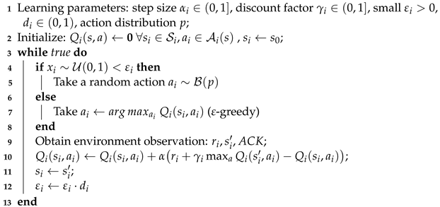
The algorithm employed by each sensor i is described in Algorithm 1. The sink gateway functions according to Algorithm 2. We define as the individual action space and state space of sensor i, respectively. Each sensor i takes action and transitions state to its next state , starting from initial state , which is the same for all sensors. All parameters are individual for each sensor i, denoting as the learning rate of sensor i, as the discount factor of sensor i, as the initial exploration probability of sensor i, and as the decay rate of sensor i. Sensors independently draw random numbers. is drawn uniformly , and the action during exploration is drawn individually as a Bernoulli trial . Both sensors and the gateway function simultaneously as each sensor needs to update its individual Q-table, denoted , and determine in each time slot whether to transmit or remain idle. The gateway sink detects whether the heard reports are interpretable and broadcasts an ACK accordingly.
| Algorithm 1: Sensor i Q-Learning for Multi-agent data-gathering WSN. |
 |
| Algorithm 2: Gateway response. |
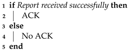 |
If no sensor performs transmission, or if more than a single sensor transmits a report during a time slot, no ACK would be broadcast.
6.1. Algorithm Complexity
The computational complexity and energy consumption associated with running multi-agent reinforcement learning (MARL) algorithms, specifically Q-learning, on sensors within the energy-harvesting wireless sensor network (EH-WSN), are critical factors to consider. Each sensor maintains a Q-table where the entries correspond to state–action pairs. The complexity of a single update cycle for one sensor, which includes action selection, action execution, and Q-value update, is . To decide upon transmission or idleness, it involves a lookup in the Q-table at the index for the current state, and chooses the action with the higher value. Since in our system, a sensor can choose from 2 actions, it is only a single mathematical operation . When the sensor updates the Q-table, according to the Q-value Equation (1), it first retrieves the current Q-value and the future Q-values for the next state , with a time complexity of and , respectively. The max operation to find also takes time. Once the exploration is complete, the arithmetic operations, including the temporal difference calculation and the update , are each. Overall, the time complexity per Q-Learning update is . Particularly, the total number of individual operations sums to 9 with 3 lookups, 1 comparison, and 5 arithmetic operations.
6.2. Memory Complexity
The space complexity for storing Q-values is , where is the number of states and is the number of actions. This is increased in size as the sensor network scales, and as the energy replenishment of the particular sensor requires a large amount of energetic states, representing more time steps charging. For example, in a network with 20 sensors, a sensor with a battery size of 40 energetic levels as its state space requires 4 bytes to represent a float value for each of the 2 possible actions: in total, a mere 320 bytes for the Q-table.
6.3. Energetic Consumption
The energy consumption for this algorithm in wireless sensor networks (WSNs) is a critical consideration that influences its practical implementation and efficiency. As detailed in Figure 3.2 in [86], the energy consumption differences between transmission (Tx) and reception (Rx) are minimal, with the most significant energy savings achieved when sensors enter a sleep state. However, our algorithm necessitates continuous updates to the Q-tables at a constant learning rate, which precludes the sensors from entering sleep mode. This inherent requirement results in less efficient energy conservation compared to protocols that allow sensors to sleep. Nevertheless, this approach is particularly suitable for energy-harvesting sensor networks, where the focus shifts from merely conserving energy to ensuring consistent energy replenishment. In these networks, sensors harvest energy from their environment, thus periodically replenishing their energy stores. This capability supports the energy demands of our algorithm, which includes continuous Q-table updates and frequent data transmissions. While our algorithm might initially seem less energy-efficient, it effectively harnesses the energy-harvesting capabilities of the network, ensuring sustained performance and reliability by maintaining an energy balance that compensates for the higher operational energy requirements.
7. Simulation and Analysis
As is known from the literature (e.g., [80]) and summarized in Section 3.2, multi-agent systems in which agents learn their policies simultaneously, without coordination or explicit sharing of learning information (such as actions, state, or Q-values) with each other, and relying on random exploratory measures to find optimality, are not guaranteed to converge to optimality due to several inhibiting factors. In the following section, we employ the use-case model described in Section 4 to highlight and analyze specific impediments that arise from transitioning from single-agent Q-Learning to the multi-agent setup. We further demonstrate how to apply certain constraints, select system parameters such as state space and reward structures, and utilize judiciously engineered algorithms to mitigate or completely eliminate these impediments. Specifically, we begin by addressing the inherent sensor behavior resulting from energy-harvesting-constrained Q-Learning. Next, we expand the setup to encompass a homogeneous multi-sensor system within different scenarios. We further extend this evaluation to include the heterogeneous sensor setup, where varying sensors exhibit different energy-harvesting rates. We then analyze the effect that random -exploration has on the resulting channel utilization and propose a networking-inspired parameter for better performance.
7.1. Simulation Preliminaries and Description
We implemented the algorithm described in Section 6 as a Python simulation. The simulation code can be found in the GitHub repository [87]. The simulation takes several algorithm parameters (e.g., discount factor , learning rate , etc.) as input, as well as the environmental setting (e.g., energy-harvesting rate , transmission energy , etc.) and network structure (number of sensors, p, etc.). Input parameters are fixed at the beginning of the simulation. During a simulation run, the multi-agent Q-Learning WSN algorithms described in Algorithms 1 and 2, are iteratively performed simultaneously on all simulated sensors and a single gateway sink.
All sensors’ simulations start simultaneously with all sensors beginning at the initial state , where each sensor possesses a full battery and their timers are reset. During the learning phase, each sensor follows the -greedy exploration policy, where an exploring agent (sensor) determines whether to transmit or remain idle at each exploratory time step, using a Bernoulli distribution. Specifically, during the exploration slot, the sensor transmits with a probability of p and remains idle with a probability of , irrespective of its current Q-table. The value of p, which determines the level of aggressiveness with which a sensor attempts to transmit during an exploration slot, is a configurable parameter that can be adjusted based on the network density. It can vary throughout the learning phase. In the ensuing simulations, we maintain a constant value of p for all sensors. The gateway sink, following Algorithm 2, responds with an ACK upon receiving a successful report. Note that in our simulations, we adopt the “errorless collision channel” model, wherein a successful transmission occurs if and only if a single sensor transmits in the corresponding time slot. All sensors perform iterative interaction and learning for a specified number of steps denoted as t. At this point, the simulation shifts from the learning phase to an evaluation phase, during which the sensors iterate over an additional time slots. During this evaluation phase, is set to 0, and the sensor’s actions rely solely on the acquired Q-values. In most of the simulated scenarios, the optimal obtainable channel utilization is easily computable. Therefore, we measure results by comparison against the best possible, i.e., the obtained network channel utilization is compared to the best possible, considering all existing constraints. We present the simulation results under different network scenarios. The following parameters were used (otherwise stated below): , initial , St.-Sp size (), and decay rate, d, which were chosen to accommodate the network size, N.
The evaluation phase spans 1000 time slots ( time slots). The results are visually presented by illustrating the status of each time slot throughout the evaluation interval. In particular, distinct colors are assigned to individual sensors, with each successful transmission during a time slot being colored accordingly. Idle slots, where no devices transmit, remain uncolored (or appear as white), while collision slots, where two or more devices transmit simultaneously, are colored black.
7.2. Sensor Inherent Constrained Behavior
To acquire insights into the projected multi-agent outcomes, we initiate this evaluation section by understanding the inherent behavior of a sensor, which stems from its inherent physical constraints. Specifically, we begin by observing the policy achieved by a single sensor that implements the Q-Learning algorithm, as outlined in Algorithm 1. It is noteworthy that this single-agent setup can be modeled as a Markov decision process (MDP), wherein the sensor attains an optimal deterministic policy. Thus, the utilization of the Q-Learning algorithm yields the anticipated optimal policy.
Figure 4 illustrates the outcomes achieved by a single sensor operating without energy constraints (top graph), i.e., the sensor is assumed to have an unlimited battery. The suggested model was adapted to this scenario by assuming no power is needed for transmission ().
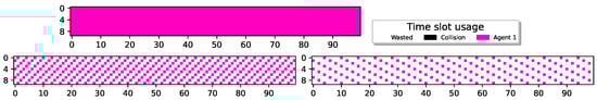
Figure 4.
Sole sensor, with no energy constraints, and with , respectively, St.-Sp , respectively, using QL.
Since the reward is based on successful reports and there are no energy constraints on the sensor, the optimal policy, as depicted in the figure, involves transmitting in every available time slot. Figure 4 also depicts the results attained by a single sensor with energy constraints, specifically (i.e., and ). It can be observed that, similar to the setup without energy constraints, the single sensor transmits whenever it accumulates sufficient power for transmission. For , the sensor transmits intermittently, based on its replenishment time. For , the sensor transmits reports every sixth slot, allowing it enough time to harvest sufficient energy for transmission. This policy aligns with the understanding that there is no benefit in delaying transmissions to a later time. Specifically, the reward for a successful transmission at time t is , whereas one time slot later, the reward for the same transmission report is discounted to where . We conclude that a sensor without external influence would exhibit a threshold policy-like behavior, pivoting at . Consequently, the sensor will never reach a full battery capacity (unless its battery is insufficient even for a single transmission, in which case it will never transmit). As a result, its state space can be truncated to encompass only its energy state .
Next, we broaden our simulations to include N sensors sharing a single channel. We examine and analyze the adaptations that an agent undergoes in its inherent sensor behavior within multi-agent settings.
7.3. Homogeneous Multi-Agent State Dis-Synchronization
Before exploring the multi-agent system, it’s important to note that the policy obtained by an isolated sensor using the Q-Learning algorithm (Algorithm 1) on an uninterrupted channel is threshold-based, with the sensor transmitting when it accumulates sufficient power. Note that applying a similar greedy policy to a multi-agent system can lead to poor performance due to collisions, where agents transmit simultaneously. For multi-agents to function effectively, they must learn to restrain from transmitting whenever they have sufficient power and learn when to remain idle.
We begin our exploration of the MAS by assuming all sensors are homogeneous, with similar charging rates and energy requirements for transmitting a report. Additionally, we assume that both of these factors are integers, allowing them to be interrelated.
Figure 5 illustrates the results for sensors with charging rates set to . It’s noteworthy that having enables all sensors to transmit reports while still leaving some slots unused, providing flexibility for each sensor in determining which slots it can transmit on.
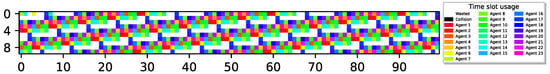
Figure 5.
23 sensors optimally align report delivery with , 76.6% utilization (best possible).
The figure shows that all sensors have learned a policy where they can transmit reports without collisions, achieving the optimal airtime utilization of 76.6% as vacant time slots are due to no sensor having enough energy for transmission.
Next, we examine a more challenging setup where , indicating that, as before, all sensors can transmit reports yet without any redundant slots, reducing flexibility. Figure 6 depicts the results for .
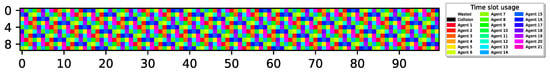
Figure 6.
21 sensors optimally align report delivery, 100% utilization.
Once again, the figure illustrates that despite the reduced flexibility, all sensors have successfully learned a policy enabling them to transmit reports in a TDMA-pattern transmission scheme, achieving 100% airtime utilization.
To better understand how different sensors with the exact same configuration, starting point, and channel perspective manage to learn different policies, we explored the Q-table. We observed that different sensors indeed have varying Q-values. Moreover, the action with the higher Q-value for the same state differs among some sensors. Consequently, their policies dictate transmission attempts on different time slots. Surprisingly, even sensors possessing identical policies and transmitting in the same energetic state manage to avoid collisions, as indicated by the fully utilized airtime. This phenomenon arises because these sensors are desynchronized regarding their energetic states; that is, the energetic state perceived by one sensor differs from that perceived by another sensor. In desynchronized energetic states, we refer to states that differ from one another by a non-integer number of the energy required to transmit a report. That is, , the energy available at state for agent i, and , the energy available at for agent j, are desynchronized energetic states at time t if for all . Note that despite all sensors initially starting from the same state, they can become desynchronized when one of the sensors reaches a full battery and refrains from attempting transmission. As a result, in the subsequent time slot, it will remain in the same state, while other sensors that have transmitted or are not in a full battery state due to earlier transmission lose synchronization with this sensor. It is also noteworthy that the probability of achieving either of the two aforementioned ways of convergence depends on the exploratory parameter p, which we separately discuss below.
We note that in both of the two aforementioned reasons for convergence to a TDMA transmission scheme—attaining different policies or reaching desynchronized energetic states—all sensors follow a threshold-type policy, similar to what is seen in a single-agent system (the inherent sensor behavior). To gain a deeper understanding of sensor behavior in this multi-agent setup, we further challenge the sensors and examine a setup in which . Note that in this setup, as sensors can recharge their batteries and transmit in cycles shorter than the number of sensors, collisions become unavoidable if the sensors continue to follow their isolated inherent behavior, maintaining a threshold-type policy, regardless of whether they attain different thresholds or find themselves in desynchronized energetic states. Figure 7 illustrates the results for and .
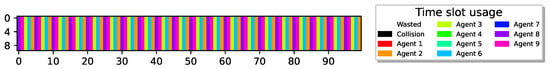
Figure 7.
9 sensors report delivery with ; 4 agents remain idle with 100% utilization; 1 M slots, .
Surprisingly, Figure 7 depicts an optimal collision-less deterministic policy that achieves channel utilization. Evidently, even though all sensors have experienced the exact same environment, different sensors have learned completely different policies. Specifically, through random exploration, some sensors experience successful transmissions and eventually learn to perform cyclic transmissions (TDMA-pattern) as before, aligning with their transmission rates. However, during their learning process, some sensors have learned to restrain their urgency to transmit, recognizing that the best possible action for the system is to remain idle due to the prevalence of unsuccessful collision experiences. Hence, the system ends up with sensors converged to two distinct policies, active and idle. In this example, one group consists of five sensors following an active policy (participating in the TDMA scheme), while the other group comprises four sensors with an idle policy (never transmitting). It is important to emphasize that this outcome is achievable due to the cooperative reward model that allows the sensor to collect rewards when other sensors succeed in transmitting a report, giving some sensors an incentive to remain idle.
In all the results presented above, optimal performance was achieved. To investigate whether optimal airtime utilization can always be learned by the sensors, we further increased the number of redundant sensors, allowing more sensors to contend for transmission. Figure 8 depicts the case for , , indicating that, in order to attain airtime utilization, almost half of the sensors should remain idle at all times.
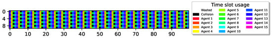
Figure 8.
15 sensors with , cyclic policy with one collision slot. Utilization of 1 M slots, .
As can be seen, similar to the results presented previously, the sensors learned a periodic behavior. However, only seven out of the eight slots in each recharging cycle are utilized successfully, while one slot is wasted due to collision, resulting in only airtime utilization. Notably, despite the high number of extra sensors, the airtime utilization is still high, and all colliding sensors converge to transmit in the same slot.
To better understand the relationship between the number of sensors (N), the sensor’s energy renewal cycle (), and the airtime utilization, we define as a measure of contending sensors. Since reaching optimal airtime utilization only requires that sensors transmit periodically, is defined as the ratio between the number of redundant sensors (the excess number of sensors over the battery renewal cycle) and the total number of sensors. Formally, . For example, in the experiment presented in Figure 8, , resulting in one cyclic collision time slot and slot utilization.
Figure 9 presents an empirical evaluation of the impact of different ratios on airtime utilization. The figure specifically depicts results for three scenarios: ( and , indicating two redundant sensors out of 40), ( and , indicating two redundant sensors out of 20), and ( and , indicating 10 redundant sensors out of 20). For each value, we conducted the experiment 100 times. The figure illustrates the average airtime utilization over these 100 runs, along with the best and worst airtime utilization observed during this set of experiments. Additionally, the figure provides insight into the convergence rate, representing the airtime utilization achieved after each 1000 iterations during the learning phase.
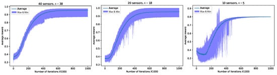
Figure 9.
Averaged reward as a function of the number of iterations. Exploratory action distribution , 1 M slots, . The graphs are averaged over 100 runs, 10 sensors with , 20 sensors with rate , and 40 sensors with rate .
We observe that in all three setups, the average reward at the end of the learning process (i.e., ) is quite high yet not optimal (not all slots were utilized successfully). Specifically, for , , for , , and for , . We observe that even in the worst runs, after convergence, at most one slot per cycle was wasted due to collision. This implies that all the redundant sensors either remained idle at all times or converged to transmit in the same time slot.
It is important to emphasize that the results presented in Figure 9 are for a specific set of parameters, including the learning rate , action distribution , initial , decay rate 99,999 and discount factor . Choosing a different set of parameters can affect performance, including convergence rate and airtime utilization. One of the parameters that significantly influences airtime utilization is the action distribution, which was fine-tuned empirically. In cases where p was set incorrectly, sub-optimal performance was observed. Nevertheless, even in these setups, relatively high performance was achieved. We delve into the determination of p in the following subsection.
7.4. Improving Performance by Adjusting Random Exploration
In this section, we advance our understanding of the learning processes in multi-agent wireless sensor networks (WSNs), focusing on enhancing the convergence towards optimal sensor policies and boosting overall network channel utilization. Building on the foundational insights presented earlier, we explore specific adjustments in learning policies and implementation to address the previously identified shortcomings. Our objective is to illustrate that despite the complexities inherent in cooperative multi-agent environments, particularly in large-scale and dynamic networks, effective solutions exist to optimize both network performance and the efficacy of the learning process.
A key aspect of this section is the examination of the impact of random exploration on network performance. Initially, all agents in the network engage in a fully random action selection, following an -greedy exploration policy with set at its maximum value of 1. This method ensures that the early phases of the learning process are governed purely by random transmission actions, constrained by the energy limits of each sensor in the network.
The core analysis here involves tracking the transition of agents from a state of complete randomness to decision-making with high performance. As the exploration rate decays, a pivotal shift occurs in the agents’ actions, moving from exploration to exploitation of learned behaviors. This transition, however, is complicated by the asynchronous nature of exploration across different agents, leading to what is termed the alter-exploration problem [62]. This issue highlights the challenge of distinguishing random actions from learned ones, until the majority of actions taken by the agents lean towards exploitation.
We rigorously analyze the balance between exploration and exploitation, and its critical role in determining the success of cooperative tasks in wireless sensor networks. At any given time slot t, each agent in the network faces a decision regarding its next action, with a probability dictating the likelihood of opting for exploration. This exploration probability is dynamically adjusted over time, decaying at a rate of . Since all N agents in the network follow a uniform learning pattern governed by an -greedy policy, the initial probability of a successful report delivery resulting from exploration actions is mathematically expressed as
where , signifying the uniform choice an agent can take at time t (transmitting and staying idle). Notice that we assume that all agents explore in unison. However, even with set to 1, this probability remains notably low and diminishes further as the network size N increases, highlighting a challenge in larger networks. To mitigate this challenge, we introduce the concept of action distribution p, modifying the probability of successful report delivery as follows:
This revised equation takes into account not just the exploration rate but also incorporates the action distribution p, thereby enhancing the probability of successful global exploration. As the number of sensors in the network escalates, the likelihood of concurrent exploration by all agents diminishes. The introduction of p serves as a compensatory mechanism to address this reduction in the probability of global exploration success during the learning process.
Further expanding this concept, we extend the analysis to scenarios where at any time slot t, a subset of m agents are exploring while the rest are exploiting. The probability of successful report delivery in such a scenario is given by
where out of N agents, m are exploring. Out of those who explore, all but one remain idle with probability p, as we assume that agents leaned the correct idle policy for time slot t.
This comprehensive formulation accounts for all possible configurations of exploring and exploiting agents within the network, providing a robust framework for understanding and optimizing cooperative success in dynamic multi-agent environments.
In the context of large-scale WSNs, the parameter p is instrumental in enhancing network performance during the exploration phase of the learning process. In such networks, the challenge is not only to learn effective policies but also to do so in a way that is scalable and efficient across a vast number of agents. Each agent’s exploration, influenced by p, impacts the overall network behavior and efficiency. When an agent is exploring, p guides the selection of actions that are more likely to result in successful report deliveries. This targeted approach to exploration, as opposed to random action selection, is particularly beneficial in large-scale networks. In these environments, the sheer number of agents can lead to a significant increase in potential action combinations and outcomes, making it more challenging to identify effective strategies. By influencing the exploratory actions to be more conducive to success, p helps agents quickly identify and reinforce beneficial behaviors, thereby accelerating the learning process. Furthermore, in large-scale networks, the probability of simultaneous exploration by all agents is low, which could lead to suboptimal learning if exploration is entirely random. With p modulating the exploratory actions, the agents are more likely to engage in explorations that are not only individually beneficial but also collectively advantageous. This ensures that the exploration phase contributes positively to the network’s overall performance, rather than leading to congestion or conflicting actions.
The reason why p is particularly effective in large-scale networks lies in its ability to reduce the inherent noise and uncertainty of exploration. In a vast network, the risk of exploratory actions leading to negative outcomes or conflicts is amplified due to the increased interactions and dependencies among agents. By guiding these explorations toward more productive paths, p minimizes this risk, ensuring that the exploration phase contributes constructively to the learning process. The parameter p can be conceptually likened to a mechanism that regulates the timing and frequency of transmissions among agents, much like the exponential back-off mechanism employed in numerous medium access control (MAC) protocols. In wireless networking, the exponential back-off mechanism is crucial for managing access to the communication medium, particularly in scenarios where multiple agents or devices attempt to transmit data simultaneously. This mechanism works by dynamically adjusting the wait time between transmission attempts, thereby reducing the likelihood of collisions and optimizing network throughput. Analogously, in our context, p functions as a strategic parameter that influences the distribution of exploratory and exploitative actions among agents within a multi-agent system. Just as the exponential back-off mechanism spaces out transmission attempts to manage channel access efficiently, p modulates transmission attempts. By adjusting p, we effectively control how frequently an agent chooses to explore new actions (akin to attempting transmissions) versus exploiting known strategies (similar to waiting or backing off). In practical terms, a lower value of p could lead to increased exploration, mirroring a scenario where agents are more aggressive in attempting transmissions, akin to a shorter back-off in traditional MAC protocols. Conversely, a higher p value means longer back-off period, where agents are more cautious and rely on established knowledge before attempting to transmit.
Figure 10 illustrates the critical relationship between the exploration action distribution parameter p and the scaling of the network. This relationship is key to accommodating an increasing number of sensors and achieving optimal learning outcomes, as demonstrated by the graph (notice that the maximum obtainable average reward is capped at 1).
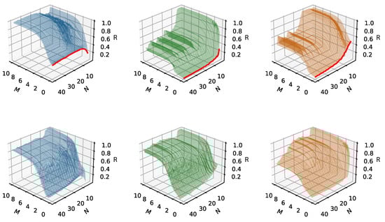
Figure 10.
Averaged reward (R) as a function of the number of sensors (N), over 10 M slots (M). Exploratory action distribution (left), (middle), (right). The graph is averaged over 10 runs. In the top row, N homogeneous sensors with . The red line represents random access with probability p. In the bottom row are N homogeneous sensors with .
Figure 10 explores the averaged reward as a function of the number of sensors, considering different values for the exploratory action distribution parameter p. These graphs provide insights into how the adjustment of p affects the learning outcomes in networks with a different scale of sensors. It demonstrates the trade-off between the level of exploration and the network scale, highlighting how a proper balance of exploration action distribution p is vital for achieving optimal learning results, especially in larger networks. At the onset of the learning process, with the initial state, and , Figure 10 depicts the impact of fully random access with a probability of . This is shown at the axis intersection, marked by a red line, corresponding to a scenario where the number of iterations is approximately zero. The graph displays how the probability of successful transmission, as in Equation (4), declines with an increasing number of sensors. The rate of this decline is influenced by , indicating that the likelihood of successful report delivery within a time slot diminishes as N increases, leading to more collisions among sensors. In this context, p can be analogized to the politeness or aggression level of a sensor’s behavior, and N represents the density or crowdedness of the network. The variation in p effectively spaces out a sensor’s random transmissions during initial exploitative phases, akin to a backoff mechanism in networking. As the Q-Learning optimization process progresses, we observe an increase in the average reward over iterations. This trend underscores the trade-off between the aggression level of sensors and their quantity. In networks with a large number of sensors, a more conservative exploration approach is required for Q-Learning to successfully attain high channel utilization. Conversely, in smaller networks, the influence of p is also evident in the resulting policies and the number of iterations required for convergence, as highlighted by the steeper slope rise when .
7.5. Algorithm Adaptiveness to Sensor Malfunction
In the previous subsection, we demonstrated that each sensor converges to a policy that achieves optimal or near-optimal overall performance. Since sensors can be inexpensive, unreliable devices prone to malfunctioning, we will now examine a scenario in which sensors may fail or new sensors may appear. It is evident that an approach that initiates a new learning process periodically or after a change has been detected will work well, assuming that the system remains stable during the learning period, similar to the setup described in the previous subsection. However, such mechanisms can be time-consuming and may result in time intervals in which, due to the repeated learning mechanism, the airtime utilization is poor with few successful reports received by the sink. The literature suggests different mechanisms for learning in the single agent setup, which adapts when the environment changes (e.g., switching between models using threshold adaptiveness [88], lifelong learning (LLL) [89], and continual RL [90]). Keeping additional policies that are learned upon for possible system changes, is costly both in memory and required learning iterations. Seldomly performing exploration where the system is converged may disrupt and temporarily reduce performance. Furthermore, while fast and efficient adaptiveness can be achieved by complex algorithms, it might not be suitable to run on simple devices.
In this subsection, we examine a different lightweight approach to facilitate the recovery of the WSN in case of the loss of one of the sensors. Essentially, the suggested approach is to let the sensors run Algorithm 1 indefinitely. Specifically, during initialization, each sensor utilizes Algorithm 1 to learn a policy, similar to what was presented in the previous section. Note that at the end of this learning period, decays to zero, while the learning rate remains constant. Despite equaling zero, indicating no exploration, the sensors continue running the learning Algorithm 1 indefinitely, i.e., they keep updating their Q-value table based on the results (rewards attained). Note that since each sensor follows a greedy policy, its policy can change in response to changes in Q-values. In the following simulations, we set the learning rate to . Sutton and Barto [83] showed that a constant performs well for a single agent), which allows the system to both converge to high Q-values in the initialization stage and react quickly to isolated failures after the policy has settled. The following Figure 11 demonstrates utilization recovery after 2 sensors simultaneously failing.
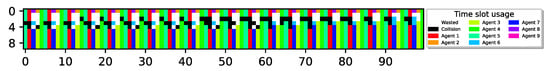
Figure 11.
2 sensors failing (agents 2 and 8) where there are 4 redundant idle sensors. Both sensors fail at , while the first policy change occurs at . The system regains full utilization at . , .
In the previous subsection, we saw that for the case of the sensors converge to a policy that is similar to TDMA, in which each sensor transmits periodically. In the case of , after the sensors converge to a policy, failure of a sensor resembles the case of a smaller N which falls under , which, as we saw, converges to the TDMA pattern. Specifically, the Q-values of all the remaining sensors of the busy slots (their own and of the other transmitting sensors) as well as the idle slots do not change and the only changes are in the new vacant slot. However, since in this setup, they have no sufficient energy for an additional transmission, and since there is no exploration to try and change the policy all over, their policy will not change. Once an active sensor ceases transmitting, which we assume is a failing sensor, a vacant slot remains unused. This free slot also results in a lack of the previously obtained reward, which in turn is reflected in the Q-values updating. Active sensors can not gain from changing their transmission policy, yet, existing idle sensors can do so. That missing reward slowly affects Q-values by reinforcing to take different action. Hence, some sensors try to transmit in order to re-maximize return. These changes in actions may result in collisions, invoking further changes in policies. Yet, at the end of this adaptation period, full utilization is obtained. However, it does not necessarily preserve any of the sensors’ policies.
In the case where a new sensor awakes and joins the network after policies have been set, it -explores, causing collisions. If no vacant slot is available, it learns an idle policy once decays to 0, as illustrated in Figure 12 (left). If a vacant slot is available, it learns the corresponding cycle to occupy it, thus increasing its gain, illustrated in Figure 12 (right).
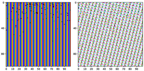
Figure 12.
Extending the evaluation period, a new sensor joins at . On the left, the system contained 8 sensors with , of which 3 learned an idle policy. The joining sensor -explores, yet learns an idle policy due to collisions accruing, whereas on the right, and all 8 sensors sparsely transmit. The joining sensor settles on one of the vacant slots. .
7.6. Influence of Data Loss and Interference
Data loss and interference are critical factors that can significantly impact the performance of wireless sensor networks (WSNs). These factors introduce challenges in maintaining reliable communication and achieving optimal network performance.
Signal loss and interference in a network of sensors can vary due to the probability of acknowledgment (ACK) loss. As the probability of ACK loss (l) increases, the expected value of the reward is affected, demonstrating how signal loss due to interference can degrade network performance. As acknowledgments are lost so too is the reward obtained by the sensors.
Figure 13 demonstrates that through ACK loss, the system maintains high utilization. The maximal possible average reward that can be obtained is depicted by a dotted line of the same color corresponding to the ACK loss probability l. For example, when the average reward is , as of the rewards are lost. A loss of an acknowledgment, either by the gateway’s misinterpretation of the transmission attempt due to noise, or as collective interference to the broadcast acknowledgment, results in a loss of reward and requires reattempts at delivering the data to the gateway sink. Nevertheless, since sensors are average learners, in which the Q-value of each sensor is averaged over all experiences, the sensors, even though not always successful, choose to transmit according to the learned policy of transmission cycles. As on average, it is still beneficial to obtain reward (less frequent than without loss) then none whatsoever. The loss’s influence is observed in the obtained Q-values, while the policy remains the same. Noise may interfere with the report data integrity; this will also result in a loss of ACK, although this can be reduced by the use of different data encoding, which supports data reliability, reducing corruption of reports due to noise.
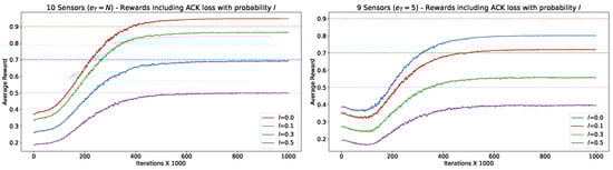
Figure 13.
Average reward during 10 M slots learning, including ACK loss with probability in a 10 sensor network with and a 9 sensor network with .
7.7. Heterogeneous Sensors with Energetic Constraint Variability
Thus far, we have dealt with homogeneous sensors. However, in wireless sensor networks, especially those relying on energy harvesting, the assumption of a homogeneous network with uniform energy-harvesting patterns for each sensor is often idealistic and does not reflect real-world conditions. The dynamics of energy harvesting in WSNs can vary considerably based on the nature of the energy source such as solar, thermal, or ambient RF energy (e.g., [91]). This variation leads to differences in the available energy for transmissions among sensors and across the network’s geographical topology [92].
In this subsection, we expand our model to include homogeneous sensors, allowing each sensor to harvest energy at a different rate. We start with a simple three-sensor setup in which the three sensors have an energy renewal cycle () of 1, 2, and 3 time slots.
As depicted in Figure 14, only sensors 1 and 3 transmit, while sensor 2 follows a policy instructing it to remain idle at all states, resulting in an overall airtime utilization of .
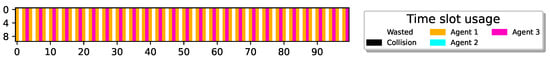
Figure 14.
St.-Sp , 3 sensors with respectively, inherent transmission cycles has no common denominator. Sensor 2 repeatedly collided with other sensors during learning, which resulted in an idle policy.
To better understand why, even in the relatively simple three-sensor setup, the sensors did not manage to converge to a policy that achieves airtime utilization, we reexamine the policies attained so far. We note that, since the state space is one-dimensional, the sensors follow a policy in which the idle sensors remain inactive at all times, while the transmitting sensors follow a cyclic pattern in which each sensor transmits periodically. Specifically, since the sensors adopt a greedy policy, each sensor transmits the first time it reaches a state in which the Q-value of the transmitting action is greater than the Q-value of the idle action, and it has sufficient energy for transmitting a report. After transmitting, the time elapsed to return to the same state is the replenishment time, making the periodic cycle of each transmitting sensor equal to the replenishment time, i.e., slots. Note that the state in which the sensor transmits can be greater than the energy required for transmission, and yet, after transmission, it will take slots to return to the same state. As long as all the sensors have the same charging rate (i.e., the same replenishment time) and, therefore, the same cyclic period, they manage to adopt a similar cyclic transmission cycle, skewed similarly to a TDMA-like pattern. However, when the sensors have different charging rates and, therefore, different periods, they need to share a common divisor to follow a TDMA-like pattern. For example, in the previous setup, if the policy attained by a sensor dictates transmission in one of the states, the sensor with a charging rate of 1 () will transmit every second slot, the sensor with a charging rate of 2 () will transmit every three slots, and the sensor with a charging rate of 3 () will transmit every four slots. Accordingly, if all three sensors transmit, the airtime utilization will be at most (the smallest common divisor is 12, so the cycle will be 12 slots). Sensors 1 and 3 can interleave their transmissions, leaving three idle slots. However, sensor 2 can only refill one such slot and will collide with the other two sensors on three slots. Hence, out of the 12-slot cycle, there are two idle slots and three collision slots, resulting in an air utilization of ). If sensor 2’s policy is to stay idle while the other two transmit, the maximal air utilization will be when they interleave their transmissions, leaving one idle slot for every four slots. When only sensors 1 and 2 transmit, the maximal air utilization will be , and if only sensors 2 and 3 transmit, the maximal air utilization will be . Consequently, as long as the three sensors follow a periodic pattern, each according to its replenishment time, the maximal airtime utilization they can achieve is , which is, indeed, the policy learned by the sensors, as depicted in Figure 14.
Accordingly, in order to enable the sensor to attain better airtime utilization, we need to devise a mechanism that breaks the bond between replenishment time and the transmission cycle. To facilitate this, we extend the previously defined state space (Section 4) and introduce a timer mechanism, termed the same-energy counter, denoted as , which tracks the duration a sensor remains fully charged.
Same-energy counter subspace: This tracks the number of consecutive time slots where the parameter has not changed. Note that since the residual energy is capped, this can only happen when the sensor is fully charged. To have a finite state space we also cap the same-energy counter subspace by F,
Specifically, is defined as follows:
Note that the F might differ among various sensors.
The combined state-space: We define the state-space (St.-Sp.) seen by each sensor by both counters described:
The state is defined by the tuple .
Note that with the additional same-energy counter, a sensor’s policy can associate a different action with the full battery state for different counter values. Accordingly, with the extended state space, a transmitting sensor’s cycle can range between and slots.
We repeat the simulations for the three-sensor setup, where the three sensors possess a different energetic replenishing cycle () of one, two, and three time slots, presented in Figure 14. The results with the extended state space, which includes the timer, are presented in Figure 15.

Figure 15.
3 sensors with state space where agents have respectively. Sensors achieve optimal channel utilization. Agent 2 elongates its transmission cycle.
It can be seen that the learned policy for sensors 1 and 3 is the same as before the addition of the same-energy counter to the state space: transmitting periodically according to their replenished time, leaving an idle slot every fourth time slot. However, sensor 2 adopts a different policy in which it remains idle for an extra time slot after the replenishment. This policy allows sensor 2 to adopt a transmission cycle of four time slots (), aligning it with the cycle of the other two sensors and specifically letting it transmit in the vacant time slot left by the other sensors, achieving airtime utilization, as illustrated in Figure 15.
We expand the heterogeneous simulation scope to include more sensors with various charging rates such that, in order to attain a cycle that resembles a TDMA pattern, some of the sensors need to stay idle at all times (). Specifically, Figure 16 depicts the results for six sensors with energetic replenishing cycles () of one, two, three, one, two, and three time slots.
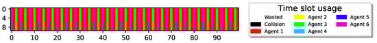
Figure 16.
6 sensors with , respectively. Agents 1, 3, and 6 with , respectively, deliver reports.
As demonstrated in Figure 16, similar to the heterogeneous setup for , the sensors are divided into two groups: those that are transmitting (sensors 1, 3, 6) and those that remain idle (sensors 2, 4, 5). For sensors in the transmitting group, the learning objective extends beyond merely desynchronizing their transmission cycles. They have also learned to adapt their transition cycles to the other sensors’ transition cycles. Specifically, sensor 1 with transmits every other time slot, while sensors 3 and 6 with restrain their transmission one slot after their battery is fully charged, adapting their cycle to sensor 1’s cycle transmitting every fourth time slot. Note that the sensors also managed to desynchronize, interleaving their transmissions and achieving airtime utilization.
We further increase the number of sensors with various replenishing rates. Figure 17 depicts the results for 15 sensors in which sensors labeled by odd index number have a replenishing rate of 25 and sensors labeled by even index number have a replenishing rate of 24.
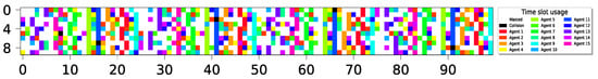
Figure 17.
15 sensors with rates 24 and 25. St.-Sp ; 5 collisions; 578 successful reports out of 600 possible; 96.3% utilization.
In the case examined in Figure 17, an optimal transmission cycle is one where all sensors’ transmissions interleave. Since sensors cannot transmit before obtaining the minimal required energetic level of a single transmission, they can only resolve to prospering transmission and elongating the transmission cycle. Optimally, all sensors with a transmission rate of 24 must elongate to a longer cycle of 25, as well as settling on a vacant time slot; 15 sensors with a transmission cycle of 25 would only be able to cyclically transmit on 15 out of 25 slots, resulting in 600 transmissions possible in the evaluated slots of Figure 17. Sensors that fail to learn the proper elongated cycle would occasionally have a single inevitable collision within this cycle with sensors of different transmission cycles. As such, in Figure 17, these transmissions may coincide with vacant slots, resulting in a relatively overall high report delivery of 578 out of 600. Despite being a seemingly simple task to learn, the fact that sensors may only transmit so seldomly, at this low transmission rate, in turn, may result in insufficient experiences to learn from. To rectify this trade-off, the learning period must be properly accommodated to suit the frequency of transmission attempts.
These findings highlight the nuanced nature of sensor behavior in energy-harvesting wireless sensor networks, particularly as the network becomes larger and more diverse, further underscoring the importance of developing adaptive learning strategies that can accommodate a wide range of operational scenarios, ensuring robust performance even as more network conditions evolve.
7.8. Comparison to Other Methods
Figure 18 shows the averaged results of 100 experiments for each value in the graphs, comparing the performance of the multi-agent reinforcement learning (MARL) approach with time division multiple access (TDMA) and slotted ALOHA under various transmission probabilities (, , and ). All experiments start from the same sensor state, leading to unique behaviors in the protocols. Notably, for slotted ALOHA with two sensors and , the transmissions align and synchronize, resulting in zero utilization due to collisions. The energy required for each transmission is . The MARL approach, being distributed, dynamically adapts to network conditions, optimizing transmission strategies and significantly outperforming slotted ALOHA across all scenarios. While TDMA consistently achieves the highest utilization due to its strict time slot allocation, in contrast, MARL offers a flexible and adaptive alternative, reducing collisions and enhancing overall network efficiency without the need for rigid time slot allocations by some centralized entity. This distributed learning capability makes MARL particularly effective in dynamic and energy-constrained WSN environments, demonstrating significant advantages over slotted ALOHA and addressing some of the limitations of TDMA.
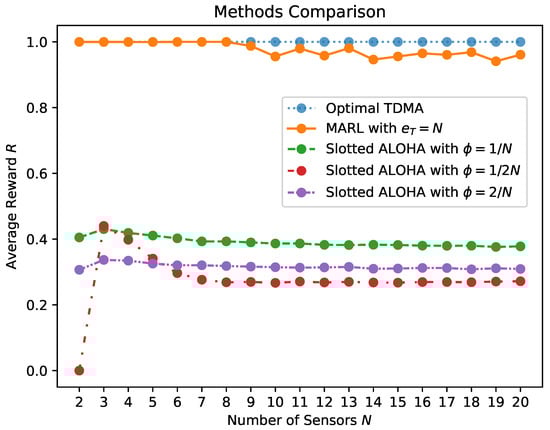
Figure 18.
A comparison of the system model with slotted ALOHA, TDMA, and MARL, where .
8. SDR Implementation
In contrast to simulation environments, where the environment is artificially programmed, hardware-based implementations experience several real-world impediments and uncertainties. For example, unlike simulations, over-the-air transmissions are exposed to impairments such as sampling noise (of both reports and ACKs), device phase noise, frequency drift, and imperfect synchronization. These factors may degrade the learning process and lead to the system failing to converge to high channel utilization.
To demonstrate the feasibility of the suggested scheme and gain insight into real-world effects, we implemented and tested the proposed learning approach on software-defined radios. Specifically, USRP B210 devices were used in a GNU radio 3.10-based multi-agent conceptual system comprising a single gateway and a few sensor nodes (Figure 19).

Figure 19.
Two-sensor and one gateway experiment setup using NI-B210 SDRs.
Figure 20 depicts the schematics of the USRP implementation. Each device employs both a receiving antenna (Rx) and a transmitting antenna (Tx). It is crucial that sensors remain synchronized, as even a slight offset in the perceived timing of the slots can lead to severe coordination issues, resulting in dramatic performance degradation. Specifically, a sensor with a time slot offset may transmit during an adjacent time slot, causing collisions with other sensors. Note that such offsets can recur both during the learning process, affecting system-wide Q-tables, and during the post-learning behavior (the adaptation of the learned policy), thereby impacting the resulting performance. Accordingly, to ensure synchronization, the gateway sink utilizes a pilot signal, which serves as a timing synchronizer indicating the beginning and the end of each time slot. This pilot signal is achieved by a single on–off frequency continuous wave (CW) generated by the GW. Although more sophisticated synchronization mechanisms exist, the simple sine wave used in our implementation was sufficient to maintain synchronization across all time slots. This sync signal is received by all sensor nodes, providing synchronized discrete timing steps to all the learning agents.
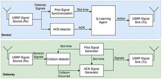
Figure 20.
General USRP implementation schematics.
For compliance with the energy-harvesting model, we implemented an artificial battery that is charged every time slot and can store at most enough energy for transmission (, respectively). Every transmission drains the battery by the equivalent of N time slots’ charging ( respectively). On each sensor, we implemented the Q-Learning agent as described in Algorithm 1. Accordingly, at each time slot indication, which marks the beginning of a new slot, each agent with sufficient energy for transmission decides whether to transmit according to the epsilon-greedy policy described in Algorithm 1. This translates to sending a CW along the channel medium to be received by the gateway sink. The gateway sink, which operates in the spirit of Algorithm 2, is calibrated to identify the signal’s energy and determine whether the transmission was made by a single agent or multiple agents (i.e., a collision). A single CW ACK signal is transmitted back to the sensor nodes whenever the GW observes that a single agent has transmitted. The sensor nodes sample this signal and deliver the ACK to the learning agent, translating it into a corresponding reward. The agent assembles experiences with this environment in the form of a tuple each time a time slot has passed and performs Q-value updates. After the exploration parameter epsilon decays and reaches a predefined threshold, the Q-value updates stop, and the agents strictly follow the learned policy.
Note some technological challenges, for example, since the sensors are deployed in various locations at varying distances from the gateway sink, they require different gains to ensure accurate reception of transmitted reports. Additionally, they need different gains and thresholds to detect ACK signals reliably. These parameters may require adjustments during the experiment due to phenomena such as fading and minor environmental changes, including movements within the experiment environment.
We ran the experiment for two topologies. The first comprises a single GW and two sensors, where the Q-value updates stopped after 2000 time slots, during which epsilon decayed to nearly zero, and the agents followed the learned policy. We further expanded the topology to include five SDRs (a single GW and four sensors), where the Q-value updates stopped after 4000 time slots. Figure 21 presents the learning process of an individual sensor for the two topologies. For comparison, the figure also depicts simulation results for the same two topologies. Since real-time environment is expected to experience some packet loss, we also added simulation results in which of the reports were randomly dropped.
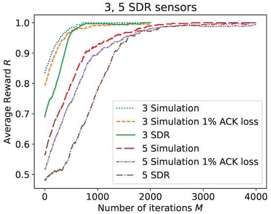
Figure 21.
Average reward for SDR and simulation with and , over slots, respectively. .
Figure 21 depicts that the final average reward converges to 1 for both topologies, indicating that all sensors transmit sequentially without empty time slots, similar to TDMA allocation. Despite real-world phenomena, the results obtained for the USRP implementation, at least for the simple two topologies, align with the simulation results. The primary distinction between the hardware implementation and the simulation lies in the convergence time. Specifically, the hardware implementation requires a longer learning phase for convergence compared to the simulation results. It is noteworthy that the simulation results with a packet drop closely resemble the implementation results, suggesting that the real-time experiments encountered report drops.
9. Conclusions and Future Research
In this study, we embarked on an ambitious journey to explore the application of cooperative multi-agent reinforcement learning (MARL) within the dynamic and complex realm of wireless sensor networks (WSNs), a crucial element in the ever-evolving landscape of big data. Our work is at the forefront of addressing the intricate challenge of efficient data gathering in WSNs, especially in environments marked by diverse constraints and dynamic conditions. The successful implementation of MARL in this context signifies a substantial leap forward, offering a potent solution to the limitations inherent in traditional data-gathering methodologies commonly used in WSNs.
Our approach harnesses the autonomous behavior of sensors within a decentralized communication framework, enabling the adaptation and optimization of data transmission strategies. This aspect is particularly pivotal under energy-harvesting constraints, where efficient resource utilization is paramount. The sensors, functioning as independent yet cooperative agents, show a remarkable ability to learn and adapt in response to the ever-changing state and requirements of the network, thereby significantly enhancing the overall efficacy of data gathering and reporting.
A considerable conclusion arising from this study is that to effectively address non-deterministic constraints, a shift towards models that can generate stochastic policies is imperative. Unlike deterministic policies, which produce a specific action for a given state, stochastic policies can incorporate a probabilistic approach, offering a range of possible actions with associated probabilities. This flexibility is crucial for adapting to the uncertainties and variabilities inherent in more complex WSN scenarios (e.g., sensors’ queue-buffered priority systems, packet loss due to varying radio fading conditions, etc.).
We also conclude that, on the one hand, this paper illustrates the potential of employing MARL in WSNs, focusing on a pervasive data-gathering application. Additionally, the results showcased here are promising, achieving optimal or near-optimal performance in many scenarios. On the other hand, it is important to acknowledge that the effectiveness of MARL can vary under different conditions. Factors such as increased sensor count, environmental randomness, dynamic topology changes, or modifications to the objective function may challenge the MARL approach and potentially lead to performance degradation.
As highlighted throughout this paper, addressing these challenges can be approached through various strategies within the Q-Learning domain, such as refining the reward function, adapting different RL algorithms, or leveraging insights from WSNs. These considerations underscore the versatility and adaptability of MARL frameworks in accommodating the diverse and evolving demands of WSN deployments.
To develop such stochastic policies, advanced tools and methodologies are required. One promising avenue is the actor–critic method, a reinforcement learning approach that combines the benefits of both policy-based and value-based methods. The actor–critic framework utilizes two models: an actor, which proposes actions, and a critic, which evaluates these actions and guides the actor. This method can effectively handle the complexities of stochastic environments, offering a nuanced approach to learning and decision making. Future research will aim to extend these approaches to encompass non-deterministic constraints in WSNs. By leveraging such tools focusing on stochastic policy generation, we can further enhance the adaptability and efficiency of wireless sensor networks. Such advancements promise not only theoretical enrichment but also practical applications in the ever-evolving landscape of wireless communications and networking.
The study also probed into the inherent challenges associated with learning in multi-agent systems, such as non-stationarity and the difficulties in synchronizing states among agents. We proposed and implemented methodologies like sequential learning and adjusting exploration patterns to overcome these hurdles, thereby enhancing the learning process and increasing the likelihood of converging to optimal strategies.
Through a combination of rigorous simulations and software-defined radio (SDR) implementations, we validated the efficacy of our proposed MARL model. These practical tests demonstrated that our approach can achieve high channel utilization and adaptability across a variety of network scenarios, even under stringent resource constraints. This not only proves the feasibility of our approach in real-world settings but also highlights the immense potential of MARL in augmenting the capabilities of WSNs.
In conclusion, our research makes a significant contribution to the field of WSNs, offering a fresh perspective on the application of MARL for data gathering. The insights and methodologies developed in this study are poised to influence future developments in WSNs, paving the way for more efficient, autonomous, and intelligent network systems. As we progress, the applications and implications of this research in the broader context of sensor networks and AI-driven communication systems are vast and hold great promise. The foundation laid by this study is expected to inspire further research and innovation in the efficient management and utilization of WSNs in various real-world applications.
Author Contributions
Conceptualization, E.D., M.S. and O.G.; Methodology, M.S. and O.G.; Software, E.D.; Formal analysis, E.D., M.S. and O.G.; Writing—original draft, E.D., M.S. and O.G.; Project administration, O.G. All authors have read and agreed to the published version of the manuscript.
Funding
This research received no external funding.
Data Availability Statement
The original contributions presented in the study are included in the article, further inquiries can be directed to the corresponding authors.
Conflicts of Interest
The authors declare no conflicts of interest.
References
- Gurewitz, O.; Shifrin, M.; Dvir, E. Data Gathering Techniques in WSN: A Cross-Layer View. Sensors 2022, 22, 72650. [Google Scholar] [CrossRef]
- Abramson, N. THE ALOHA SYSTEM: Another Alternative for Computer Communications. In Proceedings of the Fall Joint Computer Conference, New York, NY, USA, 17–19 November 1970; AFIPS ’70 (Fall). pp. 281–285. [Google Scholar] [CrossRef]
- Guravaiah, K.; Kavitha, A.; Velusamy, R.L. Data Collection Protocols in Wireless Sensor Networks. In Wireless Sensor Networks; Yellampalli, S.S., Ed.; IntechOpen: Rijeka, Croatia, 2020; Chapter 6. [Google Scholar] [CrossRef]
- Sadeq, A.S.; Hassan, R.; Sallehudin, H.; Aman, A.H.M.; Ibrahim, A.H. Conceptual Framework for Future WSN-MAC Protocol to Achieve Energy Consumption Enhancement. Sensors 2022, 22, 62129. [Google Scholar] [CrossRef]
- Lin, D.; Wang, Q.; Min, W.; Xu, J.; Zhang, Z. A Survey on Energy-Efficient Strategies in Static Wireless Sensor Networks. ACM Trans. Sens. Netw. 2020, 17, 1–48. [Google Scholar] [CrossRef]
- Braun, R.; Afroz, F. Energy-efficient MAC protocols for wireless sensor networks: A survey. Int. J. Sens. Netw. 2020, 32, 150. [Google Scholar] [CrossRef]
- Luo, H.; Huang, Z.; Zhu, T. A Survey on Spectrum Utilization in Wireless Sensor Networks. J. Sens. 2015, 2015, 1–13. [Google Scholar] [CrossRef]
- Shukla, R.; Kumar, A.; Niranjan, V. A Survey: Faults, Fault-tolerance & Fault Detection Techniques in WSN. In Proceedings of the 2022 5th International Conference on Contemporary Computing and Informatics (IC3I), Uttar Pradesh, India, 14–16 December 2022; pp. 1761–1766. [Google Scholar] [CrossRef]
- Doudou, M.; Djenouri, D.; Badache, N. Survey on Latency Issues of Asynchronous MAC Protocols in Delay-Sensitive Wireless Sensor Networks. IEEE Commun. Surv. Tutorials 2013, 15, 528–550. [Google Scholar] [CrossRef]
- Mann, M.; Singh, R. A Comprehensive Analysis of Application-Based MAC Protocol for Wireless Sensor Network. In Advanced Computing and Intelligent Technologies; Shaw, R.N., Das, S., Piuri, V., Bianchini, M., Eds.; Springer: Singapore, 2022; pp. 183–198. [Google Scholar]
- Buettner, M.; Yee, G.V.; Anderson, E.; Han, R. X-MAC: A short preamble MAC protocol for duty-cycled wireless sensor networks. In Proceedings of the 4th International Conference on Embedded Networked Sensor Systems, New York, NY, USA, 31 October–3 November 2006; SenSys ’06. pp. 307–320. [Google Scholar] [CrossRef]
- Ye, W.; Heidemann, J.; Estrin, D. An energy-efficient MAC protocol for wireless sensor networks. In Proceedings of the Twenty-First Annual Joint Conference of the IEEE Computer and Communications Societies, New York, NY, USA, 23–27 June 2002; Volume 3, pp. 1567–1576. [Google Scholar] [CrossRef]
- Polastre, J.; Hill, J.; Culler, D. Versatile Low Power Media Access for Wireless Sensor Networks. In Proceedings of the 2nd International Conference on Embedded Networked Sensor Systems, New York, NY, USA, 3–5 November 2004; SenSys ’04. pp. 95–107. [Google Scholar] [CrossRef]
- Shifrin, M.; Cidon, I. C3: Collective congestion control in Multi-Hop Wireless Networks. In Proceedings of the 2010 Seventh International Conference on Wireless On-demand Network Systems and Services (WONS), Kranjska Gora, Slovenia, 3–5 February 2010; pp. 31–38. [Google Scholar] [CrossRef]
- Sun, Y.; Gurewitz, O.; Johnson, D.B. RI-MAC: A receiver-initiated asynchronous duty cycle MAC protocol for dynamic traffic loads in wireless sensor networks. In Proceedings of the 6th ACM Conference on Embedded Network Sensor Systems (SenSys), Raleigh, NC, USA, 5–7 November 2008; pp. 1–14. [Google Scholar]
- Lu, G.; Krishnamachari, B.; Raghavendra, C. An adaptive energy-efficient and low-latency MAC for data gathering in wireless sensor networks. In Proceedings of the 18th International Parallel and Distributed Processing Symposium, Santa Fe, NM, USA, 26–30 April 2004; p. 224. [Google Scholar] [CrossRef]
- Yu, Y.; Krishnamachari, B.; Prasanna, V. Energy-latency tradeoffs for data gathering in wireless sensor networks. In Proceedings of the IEEE INFOCOM 2004, Hong Kong, China, 7–11 March 2004; Volume 1, p. 255. [Google Scholar] [CrossRef]
- Zheng, T.; Radhakrishnan, S.; Sarangan, V. PMAC: An adaptive energy-efficient MAC protocol for wireless sensor networks. In Proceedings of the 19th IEEE International Parallel and Distributed Processing Symposium, Denver, CO, USA, 4–8 April 2005; p. 8. [Google Scholar] [CrossRef]
- Mohammadabadi, S.M.S.; Yang, L.; Yan, F.; Zhang, J. Communication-Efficient Training Workload Balancing for Decentralized Multi-Agent Learning. arXiv 2024, arXiv:2405.00839. [Google Scholar]
- De Figueiredo, F.A.P.; Jiao, X.; Liu, W.; Mennes, R.; Jabandzić, I.; Moerman, I. A Spectrum Sharing Framework for Intelligent Next Generation Wireless Networks. IEEE Access 2018, 6, 60704–60735. [Google Scholar] [CrossRef]
- Singh Nayak, N.K.; Bhattacharyya, B. Machine Learning-Based Medium Access Control Protocol for Heterogeneous Wireless Networks: A Review. In Proceedings of the 2021 Innovations in Power and Advanced Computing Technologies (i-PACT), Kuala Lumpur, Malaysia, 27–29 November 2021; pp. 1–6. [Google Scholar] [CrossRef]
- Zheng, Z.; Jiang, S.; Feng, R.; Ge, L.; Gu, C. Survey of Reinforcement-Learning-Based MAC Protocols for Wireless Ad Hoc Networks with a MAC Reference Model. Entropy 2023, 25, 101. [Google Scholar] [CrossRef]
- Hussien, M.; Taj-Eddin, I.A.T.F.; Ahmed, M.F.A.; Ranjha, A.; Nguyen, K.K.; Cheriet, M. Evolution of MAC Protocols in the Machine Learning Decade: A Comprehensive Survey. arXiv 2023, arXiv:2302.13876. [Google Scholar]
- Narwaria, A.; Mazumdar, A.P. Software-Defined Wireless Sensor Network: A Comprehensive Survey. J. Netw. Comput. Appl. 2023, 215, 103636. [Google Scholar] [CrossRef]
- Zhang, C.; Patras, P.; Haddadi, H. Deep Learning in Mobile and Wireless Networking: A Survey. IEEE Commun. Surv. Tutorials 2019, 21, 2224–2287. [Google Scholar] [CrossRef]
- Praveen Kumar, D.; Amgoth, T.; Annavarapu, C.S.R. Machine learning algorithms for wireless sensor networks: A survey. Inf. Fusion 2019, 49, 1–25. [Google Scholar] [CrossRef]
- El khediri, S.; Benfradj, A.; Thaljaoui, A.; Moulahi, T.; Ullah Khan, R.; Alabdulatif, A.; Lorenz, P. Integration of artificial intelligence (AI) with sensor networks: Trends, challenges, and future directions. J. King Saud Univ.-Comput. Inf. Sci. 2024, 36, 101892. [Google Scholar] [CrossRef]
- Shahryari, M.S.; Farzinvash, L.; Feizi-Derakhshi, M.R.; Taherkordi, A. High-throughput and energy-efficient data gathering in heterogeneous multi-channel wireless sensor networks using genetic algorithm. Ad Hoc Netw. 2023, 139, 103041. [Google Scholar] [CrossRef]
- Roy, S.; Mazumdar, N.; Pamula, R. An energy optimized and QoS concerned data gathering protocol for wireless sensor network using variable dimensional PSO. Hoc. Netw. 2021, 123, 102669. [Google Scholar] [CrossRef]
- Kulin, M.; Kazaz, T.; De Poorter, E.; Moerman, I. A Survey on Machine Learning-Based Performance Improvement of Wireless Networks: PHY, MAC and Network Layer. Electronics 2021, 10, 30318. [Google Scholar] [CrossRef]
- Parsa, A.; Moghim, N.; Salavati, P. Joint power allocation and MCS selection for energy-efficient link adaptation: A deep reinforcement learning approach. Comput. Netw. 2022, 218, 109386. [Google Scholar] [CrossRef]
- Zhang, L.; Tan, J.; Liang, Y.C.; Feng, G.; Niyato, D. Deep Reinforcement Learning for Modulation and Coding Scheme Selection in Cognitive HetNets. In Proceedings of the ICC 2019—2019 IEEE International Conference on Communications (ICC), Shanghai, China, 20–24 May 2019; pp. 1–6. [Google Scholar] [CrossRef]
- Shifrin, M.; Cohen, A.; Weisman, O.; Gurewitz, O. Coded Retransmission in Wireless Networks Via Abstract MDPs: Theory and Algorithms. IEEE Trans. Wirel. Commun. 2016, 15, 4292–4306. [Google Scholar] [CrossRef]
- Aoudia, F.A.; Hoydis, J. Model-Free Training of End-to-End Communication Systems. IEEE J. Sel. Areas Commun. 2019, 37, 2503–2516. [Google Scholar] [CrossRef]
- Shifrin, M.; Menasché, D.S.; Cohen, A.; Gurewitz, O.; Goeckel, D. An SMDP approach to optimal PHY configuration in wireless networks. In Proceedings of the 2017 13th Annual Conference on Wireless On-Demand Network Systems and Services (WONS), Jackson, WY, USA, 21–24 February 2017; pp. 128–135. [Google Scholar] [CrossRef]
- Sah, D.; Amgoth, T.; Cengiz, K. Energy efficient medium access control protocol for data collection in wireless sensor network: A Q-learning approach. Sustain. Energy Technol. Assessments 2022, 53, 102530. [Google Scholar] [CrossRef]
- Geiser, F.; Wessel, D.; Hummert, M.; Weber, A.; Wübben, D.; Dekorsy, A.; Viseras, A. DRLLA: Deep Reinforcement Learning for Link Adaptation. Telecom 2022, 3, 692–705. [Google Scholar] [CrossRef]
- Guo, Z.; Chen, H. A reinforcement learning-based sleep scheduling algorithm for cooperative computing in event-driven wireless sensor networks. Ad Hoc Netw. 2022, 130, 102837. [Google Scholar] [CrossRef]
- Ding, Q.; Zhu, R.; Liu, H.; Ma, M. An Overview of Machine Learning-Based Energy-Efficient Routing Algorithms in Wireless Sensor Networks. Electronics 2021, 10, 1539. [Google Scholar] [CrossRef]
- Wang, X.; Chen, H. A Reinforcement Learning-Based Dynamic Clustering Algorithm for Compressive Data Gathering in Wireless Sensor Networks. Mob. Inf. Syst. 2022, 2022, 2736734. [Google Scholar] [CrossRef]
- Drăgan, T.A.; Tandon, A.; Strobel, C.; Krauser, J.S.; Lorenz, J.M. Quantum Multi-Agent Reinforcement Learning for Aerial Ad-hoc Networks. arXiv 2024, arXiv:2404.17499. [Google Scholar]
- Pasandi, H.B.; Nadeem, T. Challenges and Limitations in Automating the Design of MAC Protocols Using Machine-Learning. In Proceedings of the 2019 International Conference on Artificial Intelligence in Information and Communication (ICAIIC), Okinawa, Japan, 11–13 February 2019; pp. 107–112. [Google Scholar] [CrossRef]
- Yang, Z.; Yao, Y.D.; Chen, S.; He, H.; Zheng, D. MAC protocol classification in a cognitive radio network. In Proceedings of the 19th Annual Wireless and Optical Communications Conference (WOCC 2010), Shanghai, China, 14–15 May 2010; pp. 1–5. [Google Scholar] [CrossRef]
- Qiao, M.; Zhao, H.; Huang, S.; Zhou, L.; Wang, S. An Intelligent MAC Protocol Selection Method based on Machine Learning in Wireless Sensor Networks. KSII Trans. Internet Inf. Syst. 2018, 12, 5425–5448. [Google Scholar] [CrossRef]
- Amuru, S.; Xiao, Y.; van der Schaar, M.; Buehrer, R.M. To Send or Not to Send—Learning MAC Contention. In Proceedings of the 2015 IEEE Global Communications Conference (GLOBECOM), San Diego, CA, USA, 6–10 December 2015; pp. 1–6. [Google Scholar] [CrossRef]
- Park, S.H.; Mitchell, P.D.; Grace, D. Reinforcement Learning Based MAC Protocol (UW-ALOHA-QM) for Mobile Underwater Acoustic Sensor Networks. IEEE Access 2021, 9, 5906–5919. [Google Scholar] [CrossRef]
- Tomovic, S.; Radusinovic, I. DR-ALOHA-Q: A Q-Learning-Based Adaptive MAC Protocol for Underwater Acoustic Sensor Networks. Sensors 2023, 23, 4474. [Google Scholar] [CrossRef] [PubMed]
- Kherbache, M.; Sobirov, O.; Maimour, M.; Rondeau, E.; Benyahia, A. Reinforcement Learning TDMA-Based MAC Scheduling in the Industrial Internet of Things: A Survey. IFAC-PapersOnLine 2022, 55, 83–88. [Google Scholar] [CrossRef]
- Galzarano, S.; Liotta, A.; Fortino, G. QL-MAC: A Q-learning based MAC for wireless sensor networks. In Algorithms and Architectures for Parallel Processing, Proceedings of the 13th International Conference, ICA3PP 2013, Vietri sul Mare, Italy, 18–20 December 2013; Aversa, R., Kolodziej, J., Zhang, J., Amato, F., Fortino, G., Eds.; Part II; Lecture Notes in Computer Science; Springer: Berlin/Heidelberg, Germany, 2013; pp. 267–275. [Google Scholar] [CrossRef]
- De Rango, F.; Cordeschi, N.; Ritacco, F. Applying Q-learning approach to CSMA Scheme to dynamically tune the contention probability. In Proceedings of the 2021 IEEE 18th Annual Consumer Communications & Networking Conference (CCNC), Las Vegas, NV, USA, 9–12 January 2021; pp. 1–4. [Google Scholar] [CrossRef]
- lu, Y.; Zhang, T.; He, E.; Comsa, I.S. Self-Learning-Based Data Aggregation Scheduling Policy in Wireless Sensor Networks. J. Sens. 2018, 2018, 7593. [Google Scholar] [CrossRef]
- Shah, H.; Koo, I.; Kwak, K. Actor–Critic-Algorithm-Based Accurate Spectrum Sensing and Transmission Framework and Energy Conservation in Energy-Constrained Wireless Sensor Network-Based Cognitive Radios. Wirel. Commun. Mob. Comput. 2019, 2019, 1–12. [Google Scholar] [CrossRef]
- Yu, Y.; Wang, T.; Liew, S.C. Deep-Reinforcement Learning Multiple Access for Heterogeneous Wireless Networks. IEEE J. Sel. Areas Commun. 2019, 37, 1277–1290. [Google Scholar] [CrossRef]
- Al-Tam, F.; Correia, N.; Rodriguez, J. Learn to Schedule (LEASCH): A Deep reinforcement learning approach for radio resource scheduling in the 5G MAC layer. CoRR 2020, 8, 108088–108101. [Google Scholar] [CrossRef]
- Shalev-Shwartz, S. Online Learning and Online Convex Optimization. Found. Trends Mach. Learn. 2012, 4, 107–194. [Google Scholar] [CrossRef]
- Destounis, A.; Tsilimantos, D.; Debbah, M.; Paschos, G.S. Learn2MAC: Online Learning Multiple Access for URLLC Applications. In Proceedings of the IEEE INFOCOM 2019—IEEE Conference on Computer Communications Workshops (INFOCOM WKSHPS), Paris, France, 29 April–2 May 2019; pp. 1–6. [Google Scholar] [CrossRef]
- Li, G.; Cai, C.; Chen, Y.; Wei, Y.; Chi, Y. Is Q-learning minimax optimal? A tight sample complexity analysis. Oper. Res. 2024, 72, 222–236. [Google Scholar] [CrossRef]
- Li, G.; Wei, Y.; Chi, Y.; Gu, Y.; Chen, Y. Sample complexity of asynchronous Q-learning: Sharper analysis and variance reduction. IEEE Trans. Inf. Theory 2021, 68, 448–473. [Google Scholar] [CrossRef]
- Even-Dar, E.; Mansour, Y.; Bartlett, P. Learning Rates for Q-learning. J. Mach. Learn. Res. 2003, 5, 1–25. [Google Scholar]
- Busoniu, L.; Babuska, R.; De Schutter, B. A Comprehensive Survey of Multiagent Reinforcement Learning. IEEE Trans. Syst. Man Cybern. Part C Appl. Rev. 2008, 38, 156–172. [Google Scholar] [CrossRef]
- Dorri, A.; Kanhere, S.; Jurdak, R. Multi-Agent Systems: A survey. IEEE Access 2018, 6, 28573–28593. [Google Scholar] [CrossRef]
- Matignon, L.; Laurent, G.J.; Le Fort-Piat, N. Independent reinforcement learners in cooperative Markov games: A survey regarding coordination problems. Knowl. Eng. Rev. 2012, 27, 1–31. [Google Scholar] [CrossRef]
- Chen, F.; Ren, W. On the Control of Multi-Agent Systems: A Survey. Found. Trends® Syst. Control 2019, 6, 339–499. [Google Scholar] [CrossRef]
- Liang, L.; Ye, H.; Li, G.Y. Spectrum Sharing in Vehicular Networks Based on Multi-Agent Reinforcement Learning. IEEE J. Sel. Areas Commun. 2019, 37, 2282–2292. [Google Scholar] [CrossRef]
- Mota, M.P.; Valcarce, A.; Gorce, J.; Hoydis, J. The Emergence of Wireless MAC Protocols with Multi-Agent Reinforcement Learning. arXiv 2021, arXiv:2108.07144. [Google Scholar]
- Guo, Z.; Chen, Z.; Liu, P.; Luo, J.; Yang, X.; Sun, X. Multi-Agent Reinforcement Learning-Based Distributed Channel Access for Next Generation Wireless Networks. IEEE J. Sel. Areas Commun. 2022, 40, 1587–1599. [Google Scholar] [CrossRef]
- Foerster, J.N.; Assael, Y.M.; de Freitas, N.; Whiteson, S. Learning to Communicate with Deep Multi-Agent Reinforcement Learning. arXiv 2016, arXiv:1605.06676. [Google Scholar]
- Miuccio, L.; Riolo, S.; Samarakoon, S.; Panno, D.; Bennis, M. Learning Generalized Wireless MAC Communication Protocols via Abstraction. In Proceedings of the GLOBECOM 2022—2022 IEEE Global Communications Conference, Rio de Janeiro, Brazil, 4–8 December 2022; pp. 2322–2327. [Google Scholar] [CrossRef]
- Wang, B.; Gao, X.; Xie, T. An evolutionary multi-agent reinforcement learning algorithm for multi-UAV air combat. Knowl.-Based Syst. 2024, 299, 112000. [Google Scholar] [CrossRef]
- Zhou, Y.; Liu, S.; Qing, Y.; Chen, K.; Zheng, T.; Huang, Y.; Song, J.; Song, M. Is Centralized Training with Decentralized Execution Framework Centralized Enough for MARL? arXiv 2023, arXiv:2305.17352. [Google Scholar]
- Zhang, Z. Advancing Sample Efficiency and Explainability in Multi-Agent Reinforcement Learning. In Proceedings of the 23rd International Conference on Autonomous Agents and Multiagent Systems, Auckland, New Zealand, 6–10 May 2024; pp. 2791–2793. [Google Scholar]
- Tan, X.; Zhou, L.; Wang, H.; Sun, Y.; Zhao, H.; Seet, B.C.; Wei, J.; Leung, V.C.M. Cooperative Multi-Agent Reinforcement-Learning-Based Distributed Dynamic Spectrum Access in Cognitive Radio Networks. IEEE Internet Things J. 2022, 9, 19477–19488. [Google Scholar] [CrossRef]
- Sahraoui, M.; Bilami, A.; Taleb-Ahmed, A. Schedule-Based Cooperative Multi-agent Reinforcement Learning for Multi-channel Communication in Wireless Sensor Networks. Wirel. Pers. Commun. 2022, 122, 3445–3465. [Google Scholar] [CrossRef]
- Zhang, J.; Shen, F.; Tang, L.; Yan, F.; Qin, F.; Wang, C. A Multi-Agent Reinforcement Learning Approach for Dynamic Offloading with Partial Information-Sharing in IoT Networks. In Proceedings of the 2023 IEEE 98th Vehicular Technology Conference (VTC2023-Fall), Hong Kong, China, 10–13 October 2023; pp. 1–5. [Google Scholar] [CrossRef]
- Liu, L.; Ustun, V.; Kumar, R. Leveraging Organizational Hierarchy to Simplify Reward Design in Cooperative Multi-agent Reinforcement Learning. In Proceedings of the The International FLAIRS Conference Proceedings, Sandestin Beach, FL, USA, 18–21 May 2024; Volume 37. [Google Scholar]
- Park, H.; Kim, H.; Kim, S.T.; Mah, P. Multi-Agent Reinforcement-Learning-Based Time-Slotted Channel Hopping Medium Access Control Scheduling Scheme. IEEE Access 2020, 8, 139727–139736. [Google Scholar] [CrossRef]
- Geng, M. Scaling up Cooperative Multi-agent Reinforcement Learning Systems. In Proceedings of the 23rd International Conference on Autonomous Agents and Multiagent Systems, Auckland, New Zealand, 6–10 May 2024; pp. 2737–2739. [Google Scholar]
- Sohaib, M.; Jeong, J.; Jeon, S.W. Dynamic Multichannel Access via Multi-agent Reinforcement Learning: Throughput and Fairness Guarantees. In Proceedings of the ICC 2021—IEEE International Conference on Communications, Xiamen, China, 28–30 July 2021; pp. 1–6. [Google Scholar] [CrossRef]
- Nguyen, T.T.; Nguyen, N.D.; Nahavandi, S. Deep Reinforcement Learning for Multi-Agent Systems: A Review of Challenges, Solutions and Applications. CoRR 2018, 50, 3826–3839. [Google Scholar]
- Fulda, N.; Ventura, D. Predicting and Preventing Coordination Problems in Cooperative Q-Learning Systems. In Proceedings of the 20th International Joint Conference on Artifical Intelligence, San Francisco, CA, USA, 8–10 November 2007; IJCAI’07. pp. 780–785. [Google Scholar]
- Hu, R.; Ying, L. Multi-Agent Optimistic Soft Q-Learning: A Co-MARL Algorithm with a Global Convergence Guarantee. Available online: https://openreview.net/forum?id=de3bG5lPTV¬eId=o0eZ3Q9Ta6 (accessed on 1 June 2024).
- Watkins, C. Learning From Delayed Rewards. Ph.D. Thesis, King’s College, Cambridge, UK, 1989. [Google Scholar]
- Sutton, R.S.; Barto, A.G. Reinforcement Learning: An Introduction; The MIT Press: Cambridge, MA, USA, 2018. [Google Scholar]
- Watkins, C.J.; Dayan, P. Q-learning. Mach. Learn. 1992, 8, 279–292. [Google Scholar] [CrossRef]
- Williams, A.J.; Torquato, M.F.; Cameron, I.M.; Fahmy, A.A.; Sienz, J. Survey of Energy Harvesting Technologies for Wireless Sensor Networks. IEEE Access 2021, 9, 77493–77510. [Google Scholar] [CrossRef]
- Factors Influencing WSN Design. In Wireless Sensor Networks; John Wiley & Sons, Ltd.: Hoboken, NJ, USA, 2010; Chapter 3; pp. 37–51. [CrossRef]
- Dvir, E. Multi-Agent Q-Learning for Data Gathering in WSNs. 2023. Available online: https://github.com/efidvir/MA_QL (accessed on 1 June 2023).
- Chen, W.; Banerjee, T.; George, J.; Busart, C. Reinforcement Learning with an Abrupt Model Change. arXiv 2023, arXiv:2304.11460. [Google Scholar]
- Chen, Z.; Liu, B. Lifelong Reinforcement Learning. In Lifelong Machine Learning; Springer International Publishing: Cham, Switzerland, 2018; pp. 139–152. [Google Scholar] [CrossRef]
- Khetarpal, K.; Riemer, M.; Rish, I.; Precup, D. Towards Continual Reinforcement Learning: A Review and Perspectives. arXiv 2022, arXiv:2012.13490. [Google Scholar] [CrossRef]
- Prauzek, M.; Konecny, J.; Borova, M.; Janosova, K.; Hlavica, J.; Musilek, P. Energy Harvesting Sources, Storage Devices and System Topologies for Environmental Wireless Sensor Networks: A Review. Sensors 2018, 18, 2446. [Google Scholar] [CrossRef] [PubMed]
- Shaikh, F.K.; Zeadally, S. Energy harvesting in wireless sensor networks: A comprehensive review. Renew. Sustain. Energy Rev. 2016, 55, 1041–1054. [Google Scholar] [CrossRef]
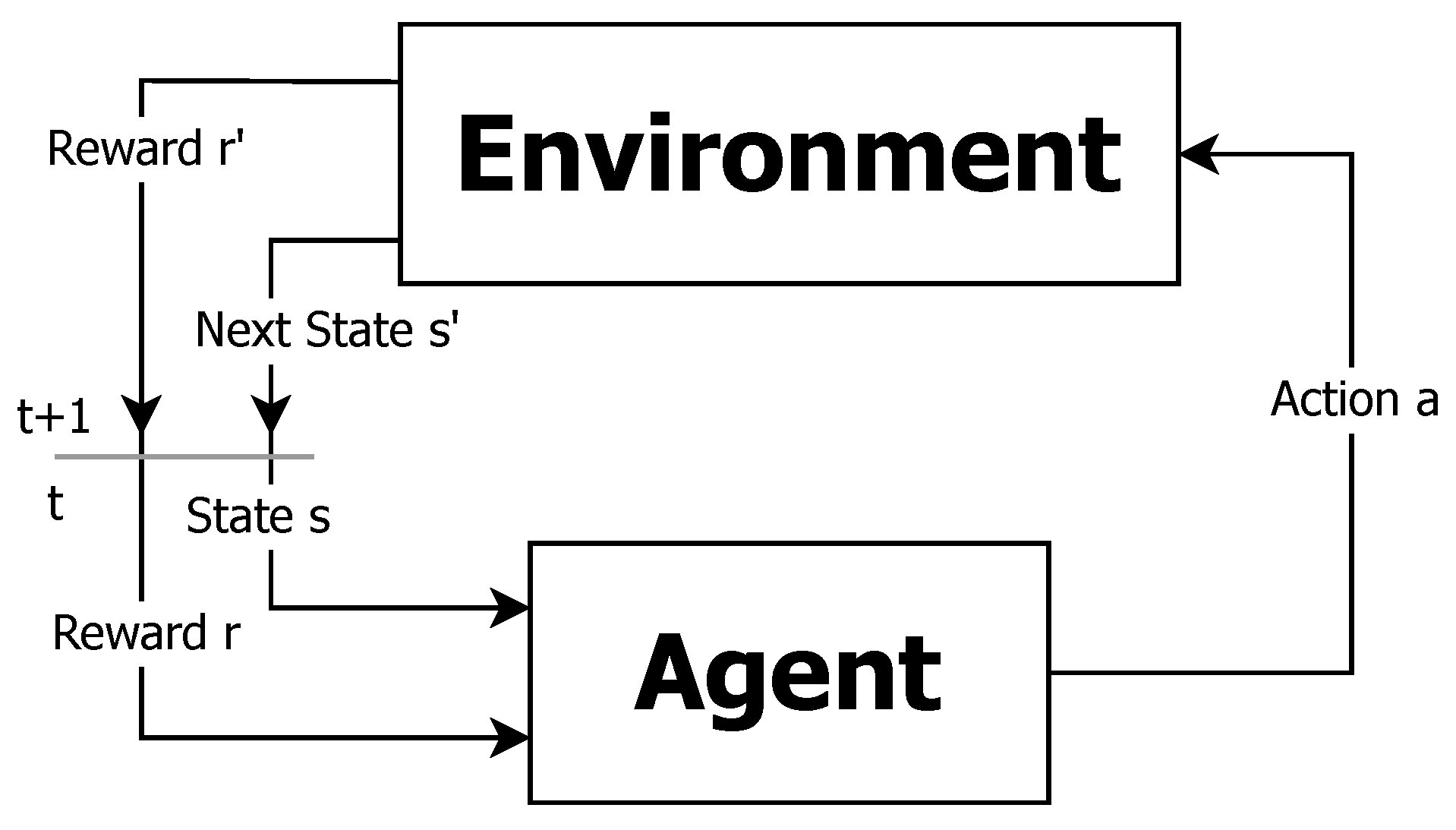

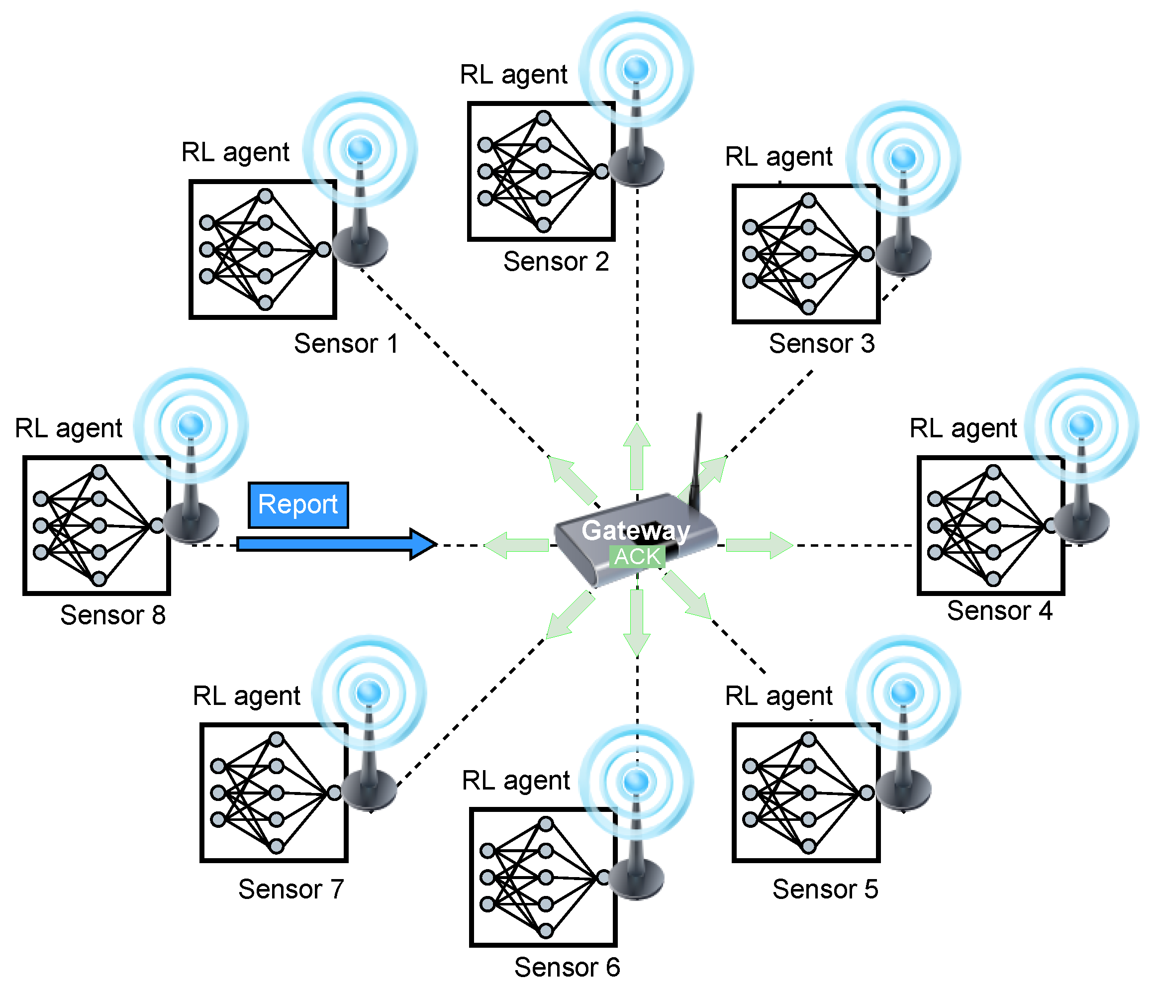


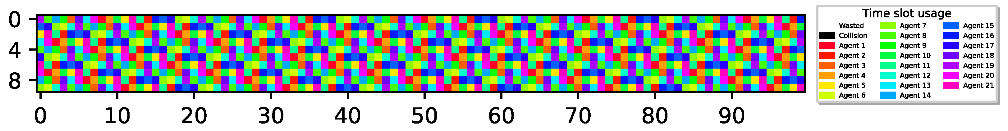
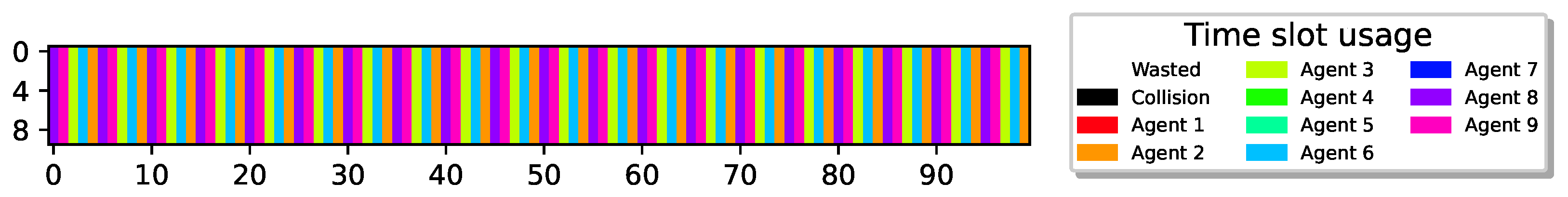
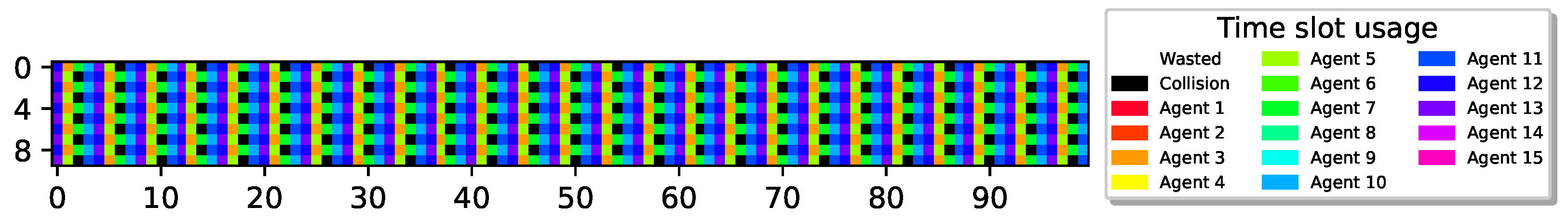
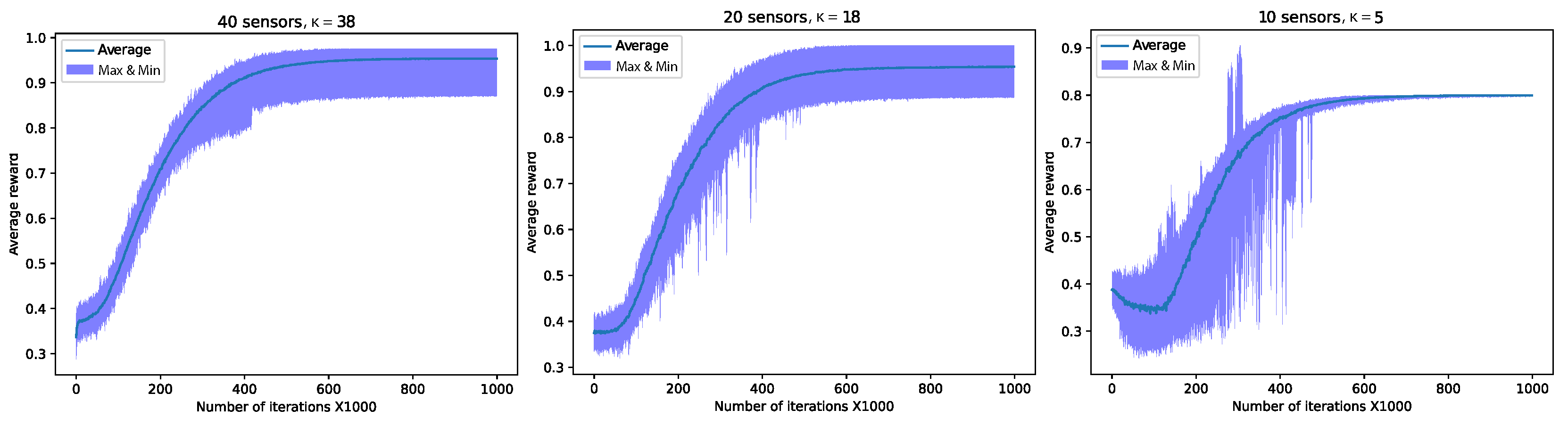
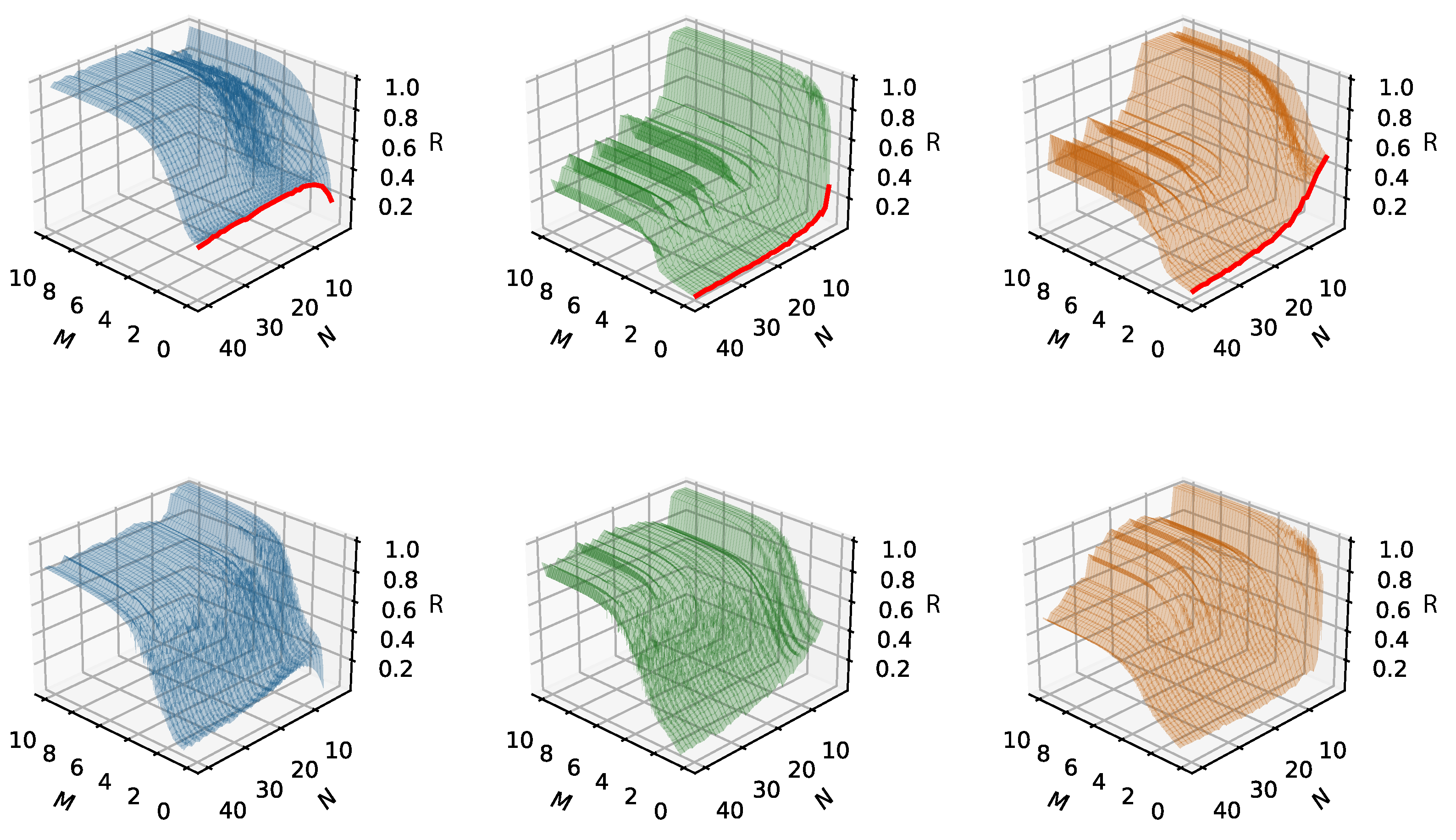

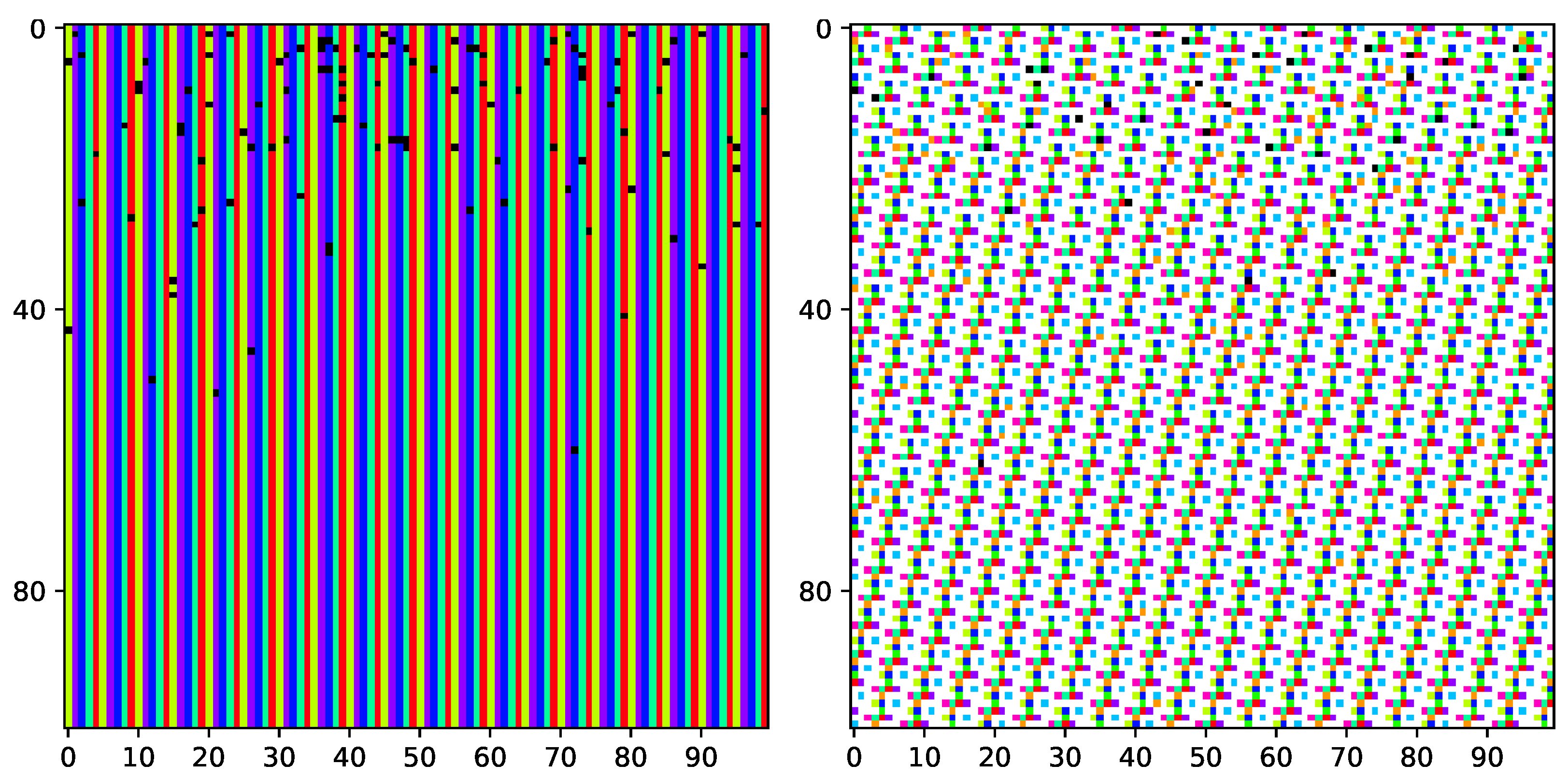
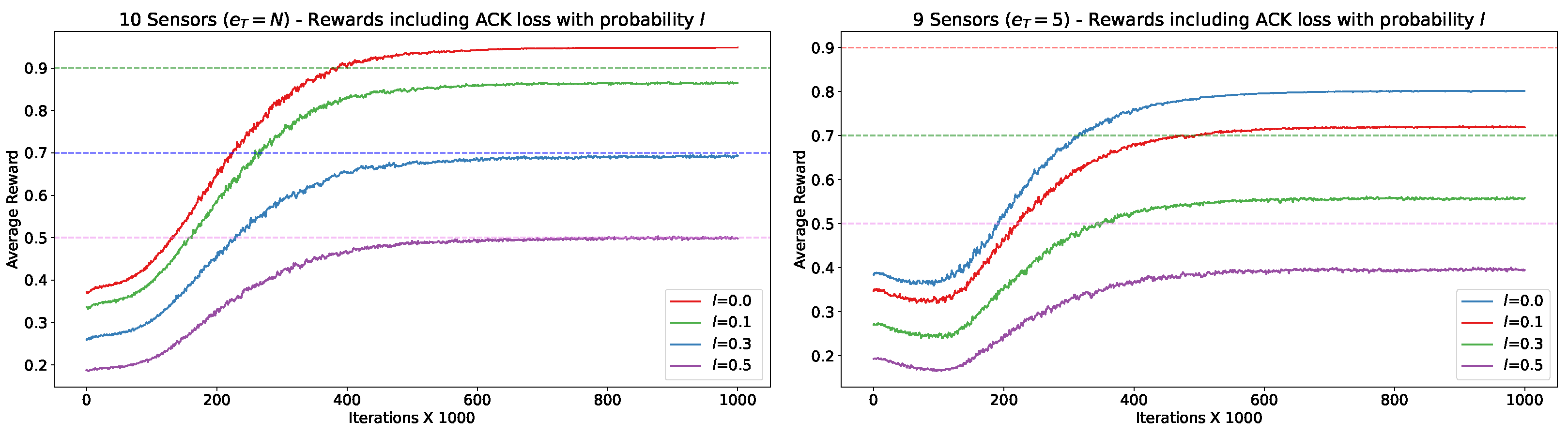
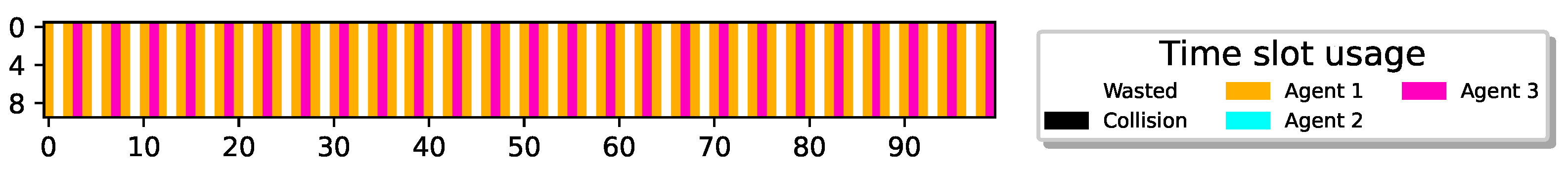
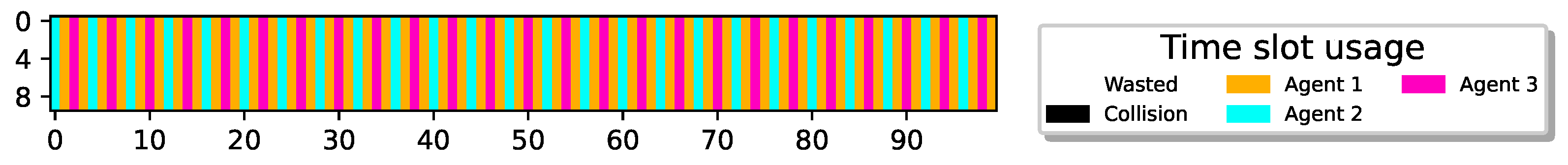

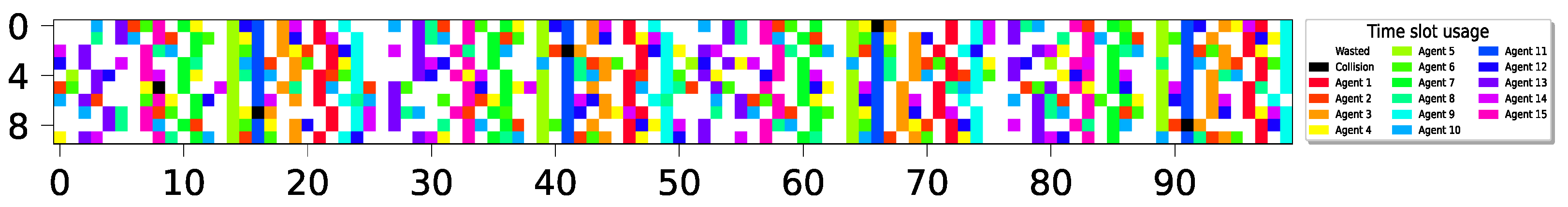
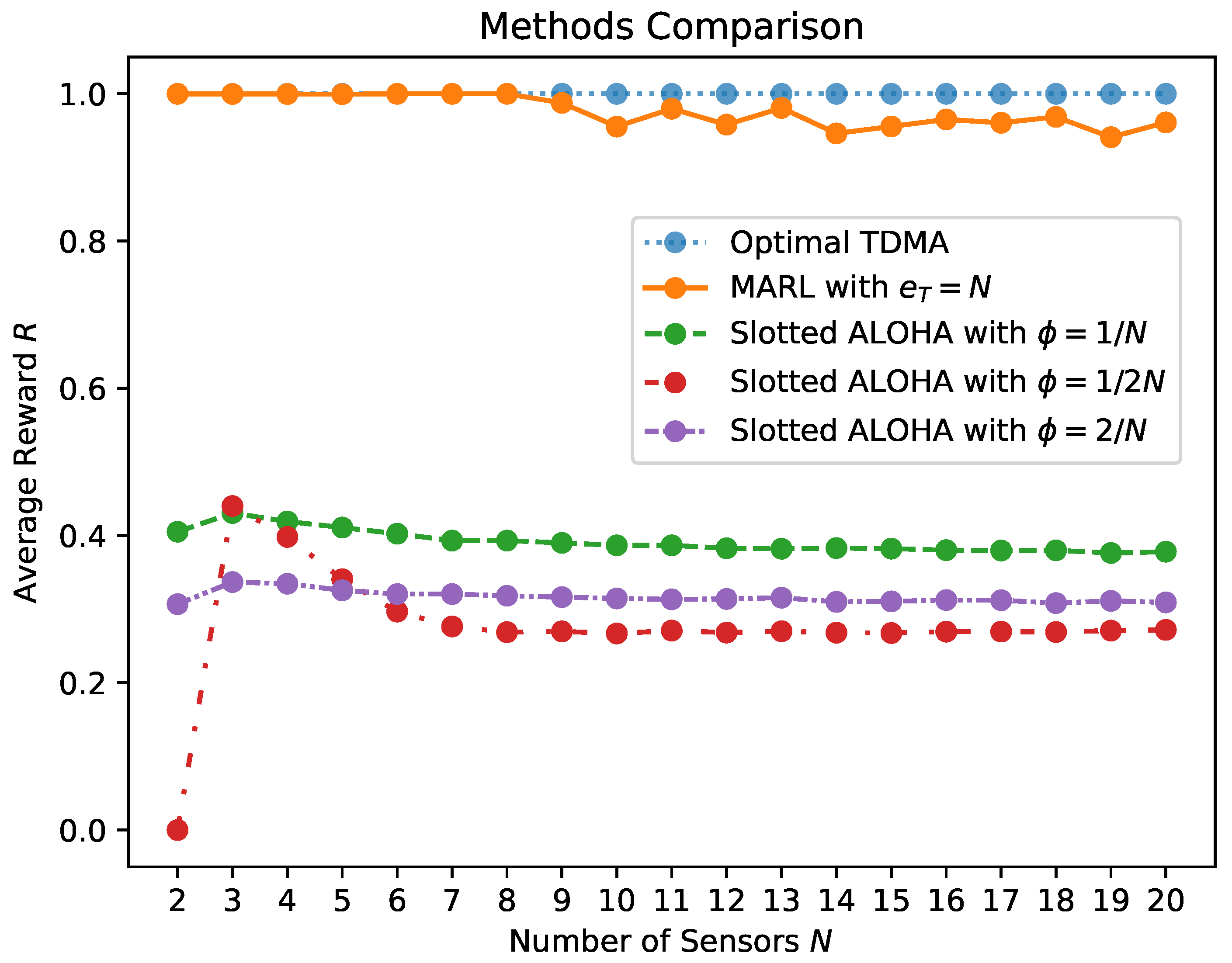

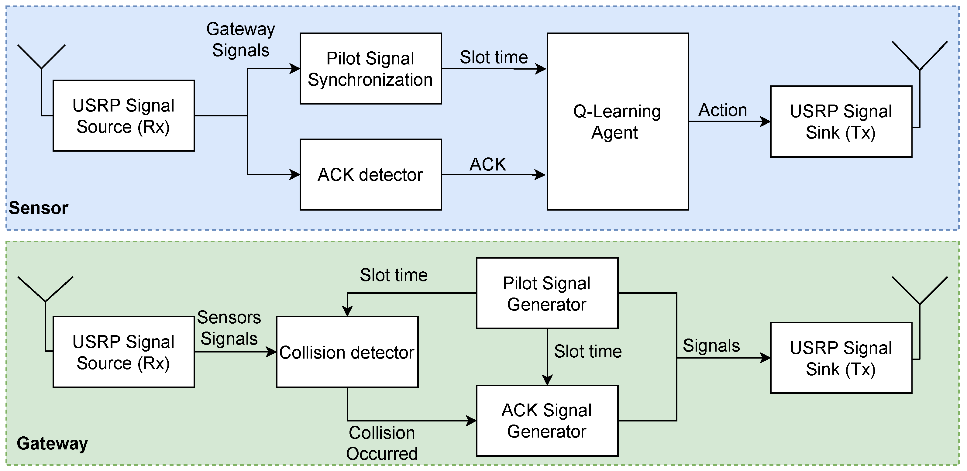
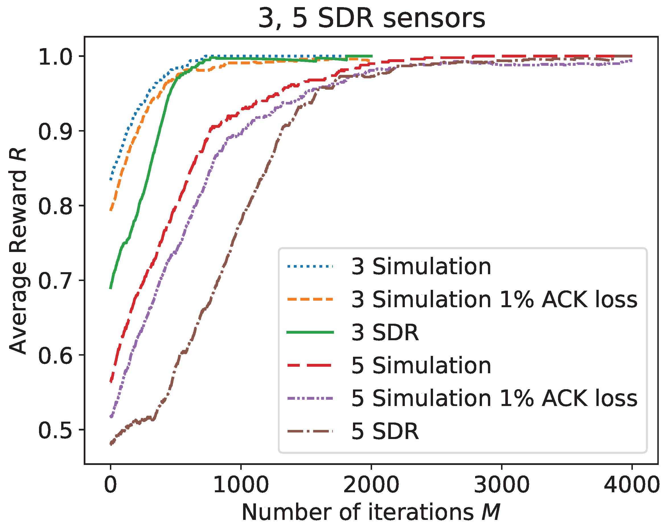
Disclaimer/Publisher’s Note: The statements, opinions and data contained in all publications are solely those of the individual author(s) and contributor(s) and not of MDPI and/or the editor(s). MDPI and/or the editor(s) disclaim responsibility for any injury to people or property resulting from any ideas, methods, instructions or products referred to in the content. |
© 2024 by the authors. Licensee MDPI, Basel, Switzerland. This article is an open access article distributed under the terms and conditions of the Creative Commons Attribution (CC BY) license (https://creativecommons.org/licenses/by/4.0/).