Abstract
The defining attribute of self-excited motion is its capability to extract energy from a stable environment and regulate it autonomously, making it an extremely promising innovation for microdevices, autonomous robotics, sensor technologies, and energy generation. Based on the concept of an automobile, we propose a light-fueled self-propulsion of liquid crystal elastomer-engined automobiles in zero-energy mode. This system utilizes a wheel comprising a liquid crystal elastomer (LCE) turntable as an engine, a wheel with conventional material and a linkage. The dynamic behavior of the self-propulsion automobile under steady illumination is analyzed by integrating a nonlinear theoretical model with an established photothermally responsive LCE model. We performed the analysis using the fourth-order Runge–Kutta method. The numerical findings demonstrate the presence of two separate motion patterns in the automobile system: a static pattern and a self-propulsion pattern. The correlation between the energy input and energy dissipation from damping is essential to sustain the repetitive motion of the system. This study delves deeper into the crucial requirements for initiating self-propulsion and examines the effect of critical system parameters on the motion of the system. The proposed system with zero-energy mode motions has the advantage of a simple structural design, easy control, low friction and stable kinematics, and it is very promising for many future uses, including energy harvesting, monitoring, soft robotics, medical devices, and micro- and nano-devices.
Keywords:
automobiles; self-excited motion; self-propulsion; liquid crystal elastomers; zero-energy mode MSC:
34C27; 37M20
1. Introduction
Self-excited motion refers to the phenomenon in which a system displays periodic motion in response to a sustained external stimulus [1,2,3]. The main characteristic of such systems is their ability to actively extract energy from a stable external environment to maintain their periodic motion [4,5]. This property greatly reduces the need for complex control systems for self-excited motion. In addition, since the amplitude and duration of the self-excited motion depend largely on the intrinsic properties of the system, such systems are highly robust [6]. The self-excited motion is inherently passive and operates autonomously without external control. This characteristic allows for a more rational system design and promotes advances in intelligence, automation, and resource efficiency, thus improving the overall effectiveness of the system [7,8]. The ubiquity of self-excited motion has led to a variety of applications in energy harvesting [9,10], power generation [11,12] sensing [13], soft robotics [14], and micro- and nano- devices [15,16].
A noticeable trend in academic literature is the growing number of studies exploring self-excited motion systems made from active materials. These materials include hydrogels [17,18], dielectric elastomers, ion gels [19], liquid crystal elastomers (LCEs) [20,21,22], and temperature-sensitive polymers [23,24]. Concurrently, significant resources have been invested in suggesting and constructing distinct self-excited motion patterns utilizing these active materials. These motion patterns include bending [23], twisting [24,25], stretching and contracting [26], rolling [27], oscillating [28,29,30], jumping [31], chaotic motions [32,33], flexible circuits [34], self-fluttering aircraft [35], engines [36,37,38] and even synchronized motion in multiple interconnected self-excited oscillators. To maintain the self-excited motion, it is typically required to apply a nonlinear feedback mechanism to compensate for energy loss from damping effects in the system [39,40]. Energy replenishment can be accomplished by various approaches, such as self-shadowing [27], coupled motion with large deformations [19], and coupled motion including air expansion and liquid column formation [41,42].
Compared to other active materials such as temperature-sensitive gels, moisture-sensitive gels, pneumatic artificial muscles, and polyelectrolyte gels, photoresponsive LCEs stand out due to their unique structural composition [43]. Recently, researchers have been focusing on the development of self-excited motion systems that utilize LCE materials [44,45,46]. LCE is a stimulus-responsive material that consists of rod-like meso-crystalline monomers with main or side chains of flexible cross-linked polymers. It combines rubbery elasticity with liquid crystal anisotropy. The liquid crystal monomer molecules exhibit rotational or phase transition behavior in response to external stimuli like electricity, heat, light, and magnetism [47,48,49,50]. This leads to a noticeable change in their overall structure, resulting in macroscopic deformation [51,52,53,54]. Compared to other active materials such as temperature-sensitive gels, moisture-sensitive gels, pneumatic artificial muscles, and polyelectrolyte gels, LCE stands out for its capacity to achieve self-sustained motion while exhibiting superior responsiveness and controllability. The exceptional reliability and consistency of self-excited motion systems based on LCE originate from the favorable properties of the LCE material, enabling wireless and non-contact actuation and control. These systems possess a broad spectrum of applications and show substantial potential in domains such as energy regulation [55,56], self-governing robotics [57,58], micro- and nano-devices [15,16], and medical devices.
Recently, a study on a light-driven self-propelled trolley was published [59]. The work introduced a novel design utilizing an LCE pendulum engine, showcasing substantial progress in the application of light energy for autonomous locomotion. In the current study, a novel self-propulsion automobile system utilizing an LCE turntable as an engine is presented. The driving force of the self-propulsion automobile is generated by the rotation of the LCE turntable engine. This technology makes lightweight propulsion automobiles possible. The rest of this document is organized as follows: Section 2 introduces a nonlinear dynamic model for the LCE turntable-engined automobile system under steady illumination. This model is based on an existing optically responsive LCE model. We also present the control equations that match this model. Section 3 involves the numerical calculations utilizing the fourth-order Runge–Kutta method. And the two motion patterns in the system and their corresponding mechanisms are examined. Section 4 explores the crucial conditions required for the system to initiate self-propulsion and how different system parameters affect the self-propulsion speed of the system and the amplitude of the mass ball in the turntable. In the last segment of the article, we provide a summary of our findings and discuss future possibilities. This study delves deeper into the crucial requirements for initiating self-propulsion and examines the effect of critical system parameters on the motion of the system. The proposed system with zero-energy mode motions has the advantage of simple structural design, easy control, reduced friction and stable kinematics, and it is very promising for many future uses, including energy harvesting and soft robotics.
2. Model and Formulation
This section describes the assembly of a propulsion automobile system engined by an optically responsive LCE turntable under steady illumination. A dynamic model of the self-propulsion automobile system with an LCE engine has been created. The focus of this section is on the control equations for the motion of the automobile system, the changes that occur in the LCE material at the molecular level, the techniques for solving the differential control equations with varying coefficients, and the process of converting the system parameters to a dimensionless form.
2.1. Dynamics of the Self-Propulsion LCE Turntable-Engined Automobile
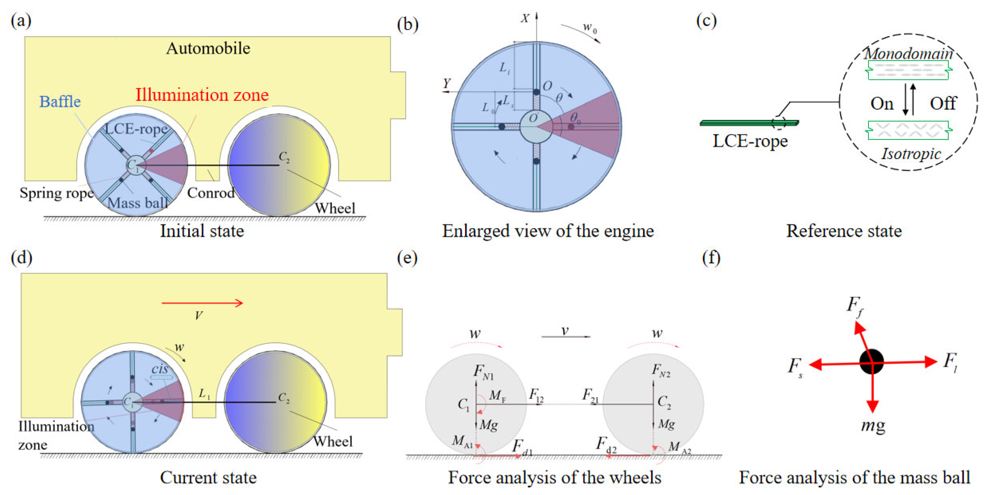
Figure 1a depicts a small self-propulsion LCE turntable-engined automobile system that includes a front wheel comprising an LCE turntable system as an engine, a rear wheel made of normal material and a linkage. The two wheels have the radius of and the mass of M, and the linkage has a length of . An illumination zone is arranged inside the LCE turntable-based front wheel, as indicated by the red region in the figure. The wheel centers and of the front and rear wheels are connected by the linkage. The friction forces between the front wheel , rear wheel , and the horizontal surface are denoted as and , generating rolling torques of and , respectively. Simultaneously, as the wheels roll, rolling damping torques and are produced between the wheels and the horizontal surface, causing the wheels to consistently rotate in the opposite direction. During the motion, the forces exerted by the linkage on the two wheels are and , respectively.
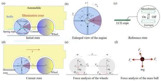
Figure 1.
Self-propulsion automobile system based on LCE turntable. (a) Initial state; (b) enlarged view of the engine; (c) reference state; (d) current state; (e) force analysis of the wheels; (f) force analysis of the mass ball. The mass ball continuously enters the heating zone and moves outward under the tension of the LCE rope. This movement creates a torque difference that allows the system to maintain a cyclic motion.
The schematic design in Figure 1b describes the internal structure of the engine, i.e., the front wheel comprising an LCE turntable-engined automobile system. It is a turntable system rotating around a point , powered by the optically responsive LCE. There are n moving tubes in the turntable. Each tube contains a tiny mass ball with a mass of m, a spring with an initial length of , and an LCE rope with an initial length of . The mass ball is located in the tube, attached to the inner side of the turntable by the spring, and connected to the outer side by the LCE rope. The mass ball is initially positioned at a distance of from the center of the turntable. In setting the light source position, we set a parallel light to illuminate the wheel vertically. In addition, we fixed a baffle to the axel, and then the regions of light and shadow remained fixed throughout the self-propulsion of the automobile. The red region, at an angle of , serves as the illumination zone. The upper limit of the illumination zone corresponds to the initial position of the turntable, and the angle between the angle between the first mass ball and the starting point is . The current length of the LCE rope is denoted by . We set the starting position of the mass ball as a reference point, created a rectangular coordinate system , and specified the initial angular velocity of the turntable in the clockwise direction.
Figure 1c depicts the optically responsiveness of LCE ropes under steady illumination. The LCE material consists of anisotropic, rod-shaped liquid crystal molecules and stretchable, long-chain polymers. This combination allows the material to reach a significant and reversible driving strain, which is mainly achieved by the transition from a nematic phase to an isotropic phase and the reorientation of the liquid crystal medium [20]. The monodomain LCE rope is produced by loosely cross-linking the mixture within a circular mold and then fully cross-linking it through uniaxial stretching and ultraviolet irradiation. The LCE rope is in a monodomain state, with the liquid crystal medium aligned along the axis. Upon entering the illumination zone, the LCE rope shrinks in its axial direction by the action of light. After leaving the illumination zone, the LCE rope fully recovers its original length. When the LCE rope does not enter the illumination zone, its length is called the reference state. Figure 1d shows the current state in which the LCE rope enters the illumination zone and the car starts to exhibit self-propulsion.
The force analysis of the wheel is illustrated in Figure 1e. Considering the momentum moment theorem as the automobile travels [60], the following control equations can be derived:
where is the moment of inertia of wheels and around the center point, represents the rotational angular acceleration of the wheels, is the driving torque, and refer to the rolling torques of the front and rear wheels, respectively, calculated as and , with and being the friction forces of the front and rear wheels against the horizontal surface, and and denote the rolling damping torques of the front and rear wheels, respectively. For simplicity, we assume that the rolling damping torques is a constant, i.e., and , in which is the rolling resistance coefficient; this value is generally determined by the wheel radius and the ground hardness [61].
Taking the direction of wheel motion as the positive direction, the following equilibrium equations can be obtained by analyzing the forces on the two wheels in the horizontal direction:
where and are calculated as the forces between the two wheels, and are the friction forces of the front and rear wheels against the horizontal surface, and is the translational acceleration of the wheels, calculated as , and .
Inside the LCE turntable-based front wheel , the wheel starts to move due to the electrothermal contraction of the LCE rope. Given the previous model of the electrothermally driven LCE turntable-engined automobile system, the driving torque applied to the whole system can be derived from the following equation:
where denotes the damping factor, is the gravitational acceleration, indicates the displacement of the -th mass ball, is the rotational angle of the wheel and represents the rotational angular velocity of the wheel.
As described in Figure 1f, when the motion tube enters the illumination zone, the LCE rope experiences a light-driven contraction, pulling the mass ball towards the outside of the turntable. The displacement moved by the mass ball is recorded as , which generates a gravitational torque difference to promote the rotation of the system. The mass ball enters the illumination zone and is subjected to four forces, i.e., the elastic force from the spring, the tension from the LCE rope, the gravity of the mass ball itself, and the damping force . Assume that gravity is negligible relative to the elastic force. Since the mass ball is in equilibrium at any moment in the X-axis direction, we can obtain its equilibrium equation as
In accordance with Hooke’s law [62], we have
where refers to the elastic stiffness of the spring, refers to the elastic stiffness of the LCE rope, and is the photothermally driven contraction strain of the LCE rope.
Inserting Equation (5) into Equation (4) yields
The light-driven contraction strain of the LCE rope can be calculated as
where is the temperature change in the LCE rope, and is the thermal contraction coefficient of the LCE rope.
Combining the rolling damping torque of the front wheels and the rolling torques of the rear wheels, denoted as and ,
Substituting Equations (2), (8) and (9) into Equation (1) and simplifying, we obtain
Substituting Equations (4)–(7) into Equation (10) and simplifying, we obtain the control equations of the system:
where is the self-propulsion speed.
2.2. Photothermally Responsive LCE Rope Model
This section details the method for calculating the temperature in Equations (6) and (7) by establishing the photothermally responsive LCE rope model. During the self-rotation of the LCE-based engine, heat exchange occurs between the LCE rope and the environment. We assume that the radius of the LCE rope is significantly smaller than its length . For typical values of the heat transfer coefficient, and considering the simultaneous transition of the LCE rope into illuminated or non-illuminated states, the temperature along the longitudinal direction is assumed to be uniform. Under steady illumination, the temperature of the LCE rope is governed by
where refers to the specific heat capacity, indicates the heat transfer coefficient, and represents the heat flux from the steady illumination.
By solving Equation (13), it can be observed that in the illuminated zone, the temperature in the LCE rope, which transitions from the nonilluminated state with a transient temperature , is given by
where denotes the limiting temperature difference in the photothermally responsive LCE rope in the illumination zone, and is the duration of current process. is the characteristic time of heat exchange between the LCE rope and the environment, and the larger is, the longer the time required for the LCE to reach the limiting temperature difference .
In the dark zone, the temperature in the LCE rope, transitioning from the illuminated state with a transient temperature , can be derived from Equation (13) as
where is the duration of current process.
2.3. Nondimensionalization and Solution Method
For convenience, the dimensionless quantities are introduced as follows: , , , , (where is the environmental temperature), , , , , , , , , , , , and . Re-substituting the above dimensionless parameters into the aforementioned Equations (3) and (6) yields the dimensionless control equations
where and represent the dimensionless rotational angular acceleration and velocity of the wheel, respectively.
The initial conditions of the system are given as
Here, we take into account the dimensionless parameters, including , , , , , , , , , , and . To address these intricate differential equations featuring variable coefficients, we employ the fourth-order Runge–Kutta method for numerical computation within MATLAB R2016b software. In the calculation, for the temperature and the position of mass ball at time , the current contraction strain of the LCE rope and the driving torque can be determined from Equations (3) and (7). Then, the mass ball position at can be calculated from Equation (12). Meanwhile, the current temperature is determined to estimate the temperature from Equations (14) and (15). Thus, the current rotational angular velocity can be calculated from Equation (17). When , the mass ball is within the illumination zone, otherwise, it is in the dark zone. Repeating the above process, the time course of the rotational angle is obtained via iterative calculation.
3. Two Motion Patterns and Mechanism of Self-Excited Motion
In this section, we will make use of the previously established control equations and perform numerical analyses in order to explicitly study the dynamic behavior of the system under steady illumination. Firstly, we will introduce the two main motion patterns, i.e., the static pattern and the self-propulsion pattern. Next, we will explore the mechanism of the self-excited motion, providing insight into the system parameters associated with each motion pattern.
3.1. Two Motion Patterns
In order to examine the problems associated with the LCE turntable-engined automobile system, it is crucial to initially ascertain the dimensionless parameters inside the theoretical model. Following the available experimental data [63,64,65], the material properties, geometric parameters, and relevant dimensionless parameters of the system are specified in Table 1 and Table 2. Table 1 provides a clear and detailed overview of the basic material properties and geometric measurements of the system. Referring to the related experimental works [20], the values for the modulus and shrinkage coefficient of the LCE rope used in the numerical simulations are determined. Table 2 displays the associated dimensionless parameters, which are calculated from the fundamental data depicted in Figure 1 and the corresponding dimensionless equations. This study will utilize these parameter values to evaluate the self-propulsion features of the LCE turntable-engined automobile system under steady illumination.

Table 1.
Material properties and geometric parameters.
Table 2.
Dimensionless parameters.
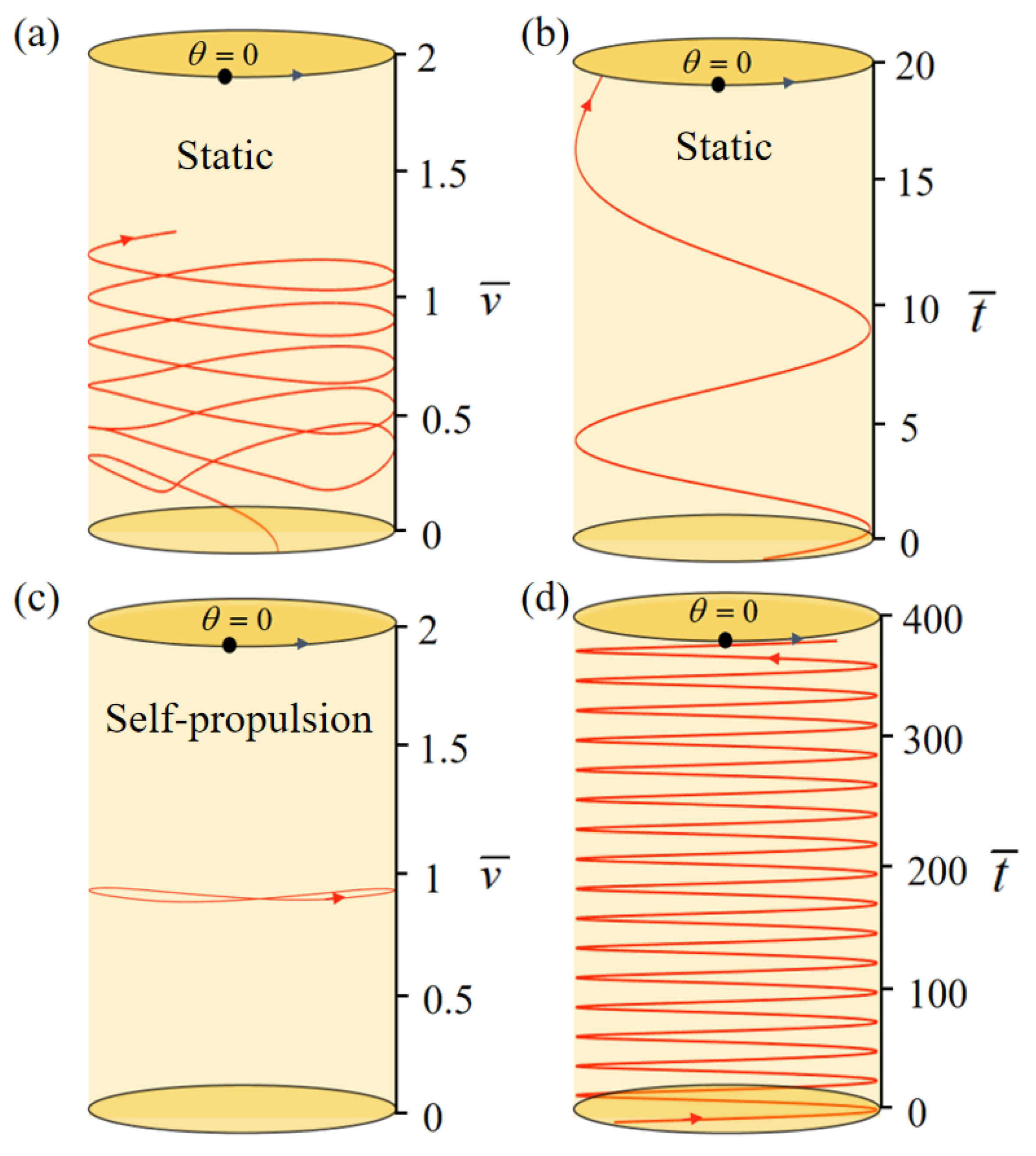
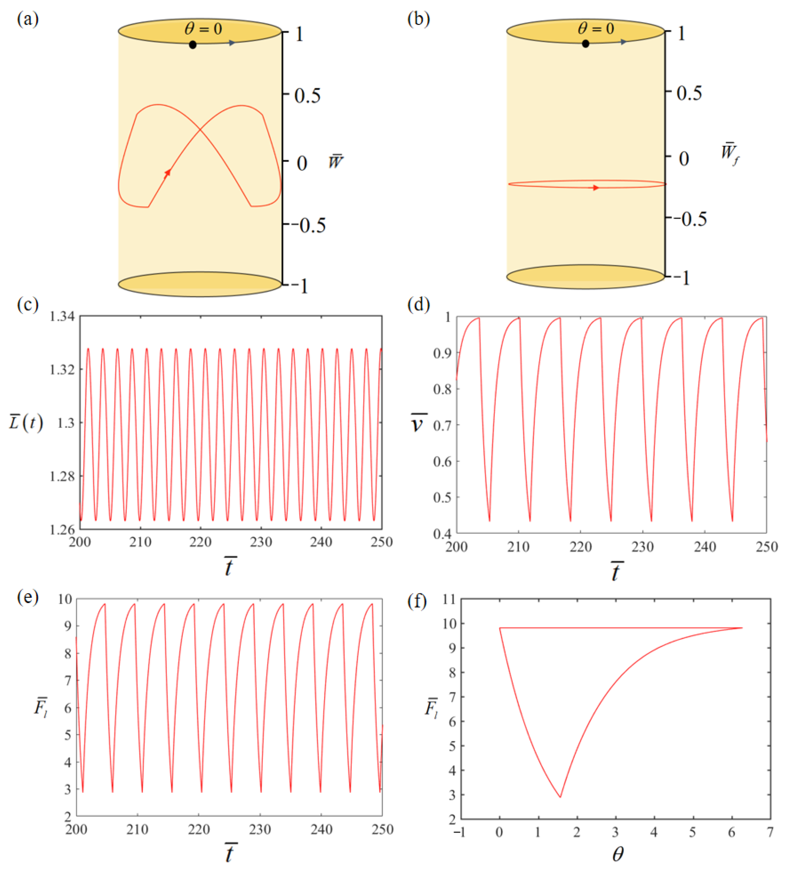
According to Equations (16) and (17), the phase trajectory and time course of the LCE turntable-engined automobile system under steady illumination can be obtained. We first set , , , , , , , , , , and . With this group of parameters, the turntable begins to rotate with an initial angular velocity of . Since indicates that the system is in the dark zone, the LCE rope does not change, and the turntable continues to rotate. Due to damping, the self-propulsion speed of the system decreases and eventually stabilizes, which is the static pattern displayed in Figure 2a,b. When the parameters are set to , , , , , , , , , , and , as depicted in Figure 2c,d, the system can continue to advance and eventually develop into a self-propulsion pattern. Similar to other self-excited motion systems, the LCE turntable-engined system can also perform propulsive motion under steady illumination. This phenomenon is mainly due to the fact that the external energy input offsets the damping losses, thus maintaining self-propulsion. The complex mechanism underlying this self-propulsion pattern is explored in depth in Section 3.2.
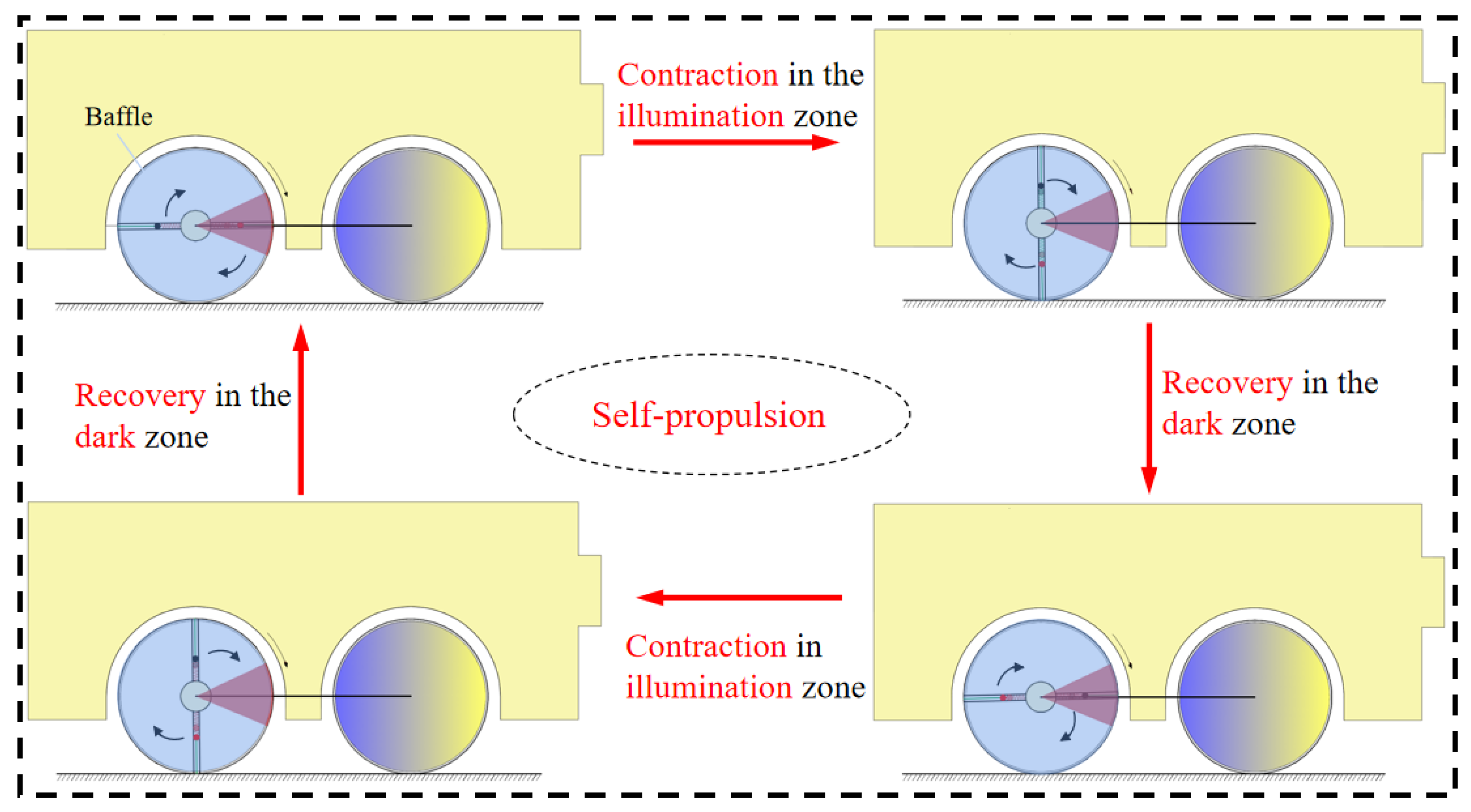
3.2. Mechanism of Self-Propulsion
Figure 3 illustrates the variations in several important parameters associated with the self-propulsion presented in Figure 2c,d, which aids in the understanding of its mechanism. Figure 4 depicts the motion of the self-propulsion system throughout one cycle. Figure 3a,b plot the correlation between driving torque, damping torque, and rotation angle, respectively. The region bounded by the two curves symbolizes the combined effect of the driving torque and the system damping, resulting in a network of 0.236. The positive network performed by the driving torque counteracts the energy dissipated by the damping, allowing the system to sustain a consistent and stable rotational motion. Figure 3c,d display the time variations in the LCE rope length and the self-propulsion speed of the automobile system, respectively. In Figure 3c,d, the wheel’s rotational speed depends on the deformation speed of the LCE rope, indicating that the two variables are interdependent. By adjusting the relevant parameters, we can control the deformation speed of the LCE rope, thereby regulating the rotational speed of the wheel. Both quantities exhibit periodic variations over time. Figure 3e,f illustrate the correlation between the tension of the LCE rope and time and rotational angle, respectively. It is evident that the tension also exhibits periodic variations in a similar manner.

Figure 3.
(a) Driving torque as a function of rotation angle; (b) damping torque as a function of rotation angle; (c) time dependence of LCE rope length; (d) time dependence of self-propulsion speed; (e) time dependence of tension of LCE rope; (f) tension of LCE rope as a function of rotation angle.
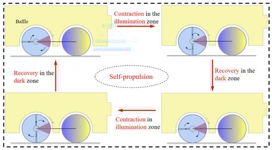
Figure 4.
Self-propulsion of the automobile system over a one cycle under the conditions of Figure 2c,d. Under steady illumination, the automobile system will exhibit continuous forward self-propulsion.

Figure 2.
Time courses and phase trajectories of the LCE turntable-engined automobile system. (a,b) Static pattern with parameters of , , , , , , , , , and . (c,d) Self-propulsion pattern with parameters of , , , , , , , , , and . The LCE turntable-engined automobile system involves two motion patterns under steady illumination, namely, static pattern and self-propulsion pattern.
3.3. Critical Condition for the Self-Propulsion
According to the self-propulsion mechanism discussed in Section 3.2, the driving torque must exceed the starting, rolling, damping torque for the system’s propulsion to be triggered. When the system starts to be illuminated from rest, with the increasing irradiation time, the mass block of the illuminated area continuously moves outward, and the driving moment keeps increasing. Combining Equations (3), (6) and (13), the maximum driving moment corresponding to the infinite irradiation time can be obtained as
where
Therefore, the critical condition for the self-rotation can be written as:
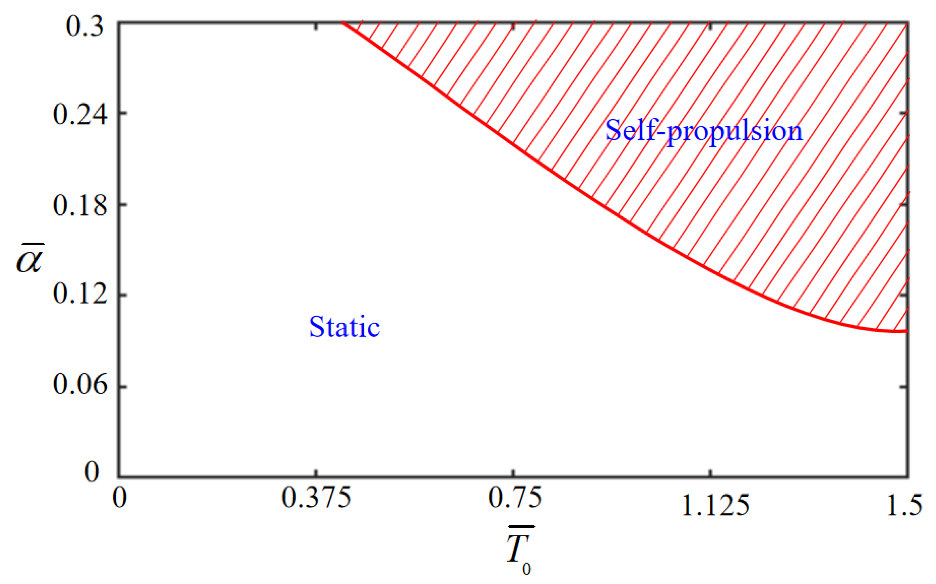
Equation (21) provides the critical condition for the self-propulsion of the LCE turntable-engined automobile system. It can be seen that the critical condition is related to , , , , , , , and , but has no relations with and . Based on Equation (21), Figure 5 plots the phase diagram of the LCE turntable-engined automobile with respect to the limit temperature and thermal contraction coefficient at , , , , , , , and . When the combination of limit temperature and thermal contraction coefficient is in the shaded region, the LCE turntable-engined automobile can propel itself periodically and continuously; otherwise, it will remain stationary.
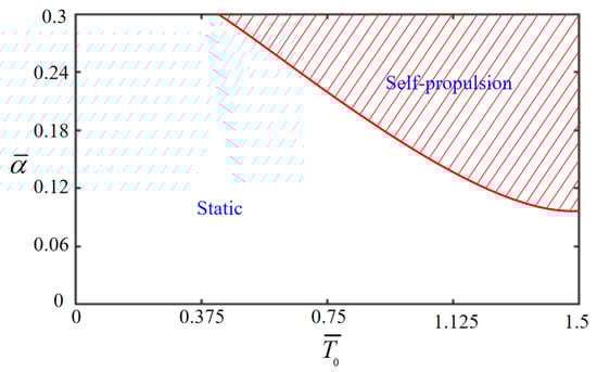
Figure 5.
Phase diagram of LCE turntable-engined automobile with respect to limit temperature and thermal contraction coefficient for , , , , , , , and . When the combination of limit temperature and thermal contraction coefficient is in the shaded region, the automobile can self-propel in a periodic and continuous fashion; otherwise, it remains static.
4. Parametric Study
The considered equations involve nine dimensionless parameters: , , , , , , , and . These parameters play a crucial role in modulating the dynamics of the LCE turntable-engined automobile system, as illustrated in Figure 1. This section aims to investigate the critical conditions for the self-propulsion motion of the automobile system with only two mass balls in the LCE turntable, and to focus on the effect of key parameters on it. The objective is to provide insights applicable to various domains such as energy harvesting [9,10], power generation [11,12], sensing [13], soft robotics [14], and micro- and nano-devices [15,16]. Here, represents the self-propulsion speed of the automobile system, and A represents the dimensionless motion amplitude of the mass ball in the LCE turntable.
4.1. Effect of Gravitational Acceleration
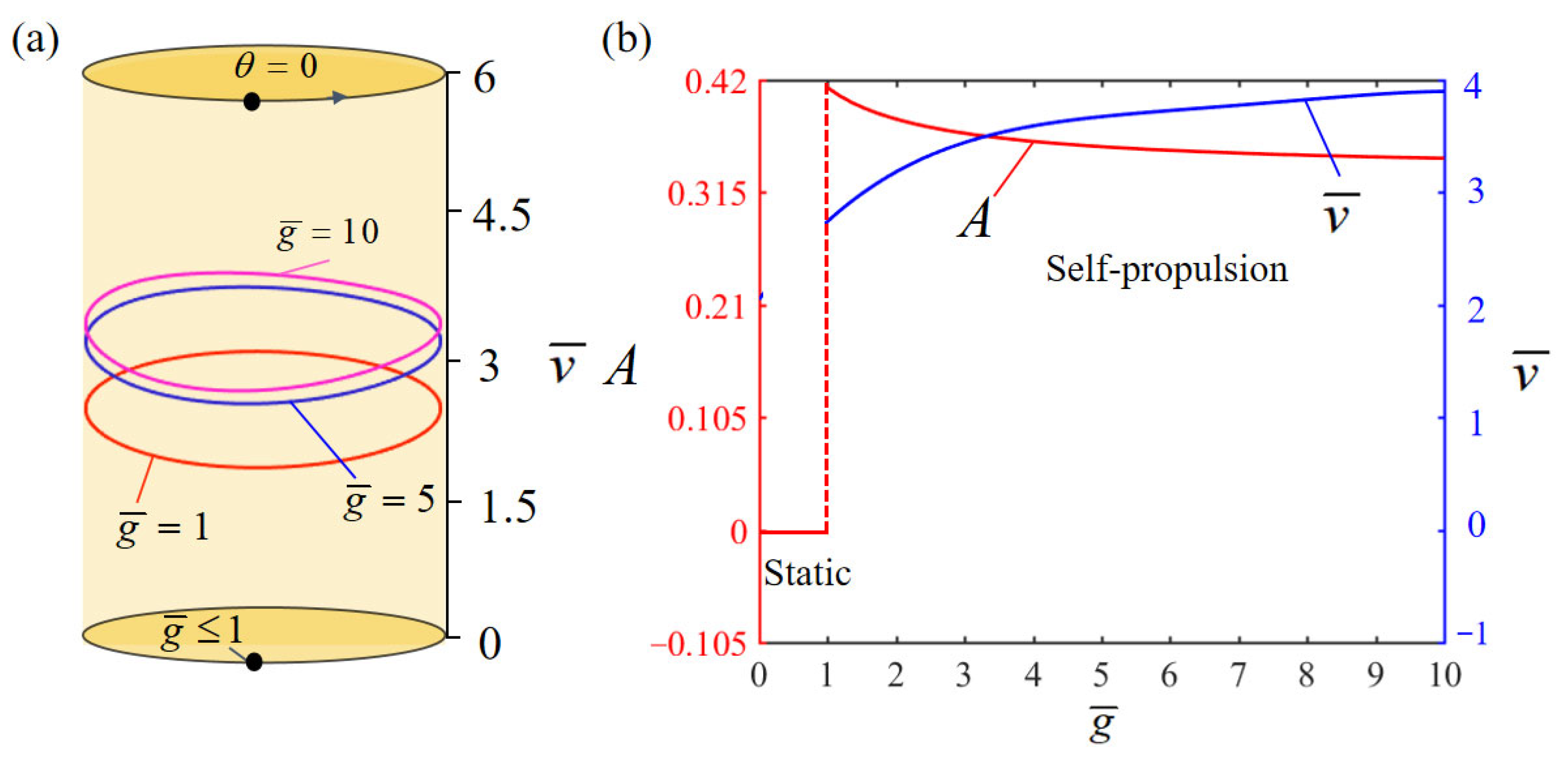
Figure 6 illustrates the effect of gravitational acceleration on the self-propulsion of the system. In the numerical calculation, the other parameter values are set as , , , , , , , , , and . Figure 6a plots the limit cycles at different gravitational accelerations. There exists a critical threshold of gravitational acceleration with a value of that triggers the rotation of the LCE engine, leading to the self-propulsion of the LCE turntable-engined automobile system; this is also consistent with the critical value calculated by Equation (21). This threshold marks the entry of the system into self-propulsion pattern, which can be explained in terms of energy balance. When the gravitational acceleration is low, the system can only generate a small amount of driving torque in the illumination zone; thus, the net energy transferred to the LCE turntable is insufficient to offset the energy loss due to damping. Consequently, the LCE turntable-engined automobile system eventually stops moving and enters a static equilibrium state, at which point the energy input is not able to offset the damping losses. In addition, Figure 6b describes how different gravitational accelerations affect the self-propulsion speed of the system as well as the motion amplitude of the mass ball in the LCE turntable. The self-propulsion speed of the system increases with the increasing gravitational acceleration, while the amplitude of the mass ball decreases and then stabilizes.
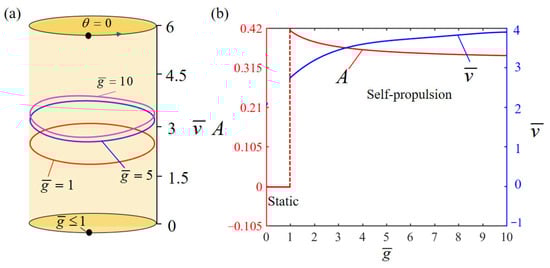
Figure 6.
Effect of gravitational acceleration on the self-propulsion of the system, with , , , , , , , , , and . (a) Limit cycles; (b) self-propulsion speed and mass ball amplitude.
4.2. Effect of Limit Temperature
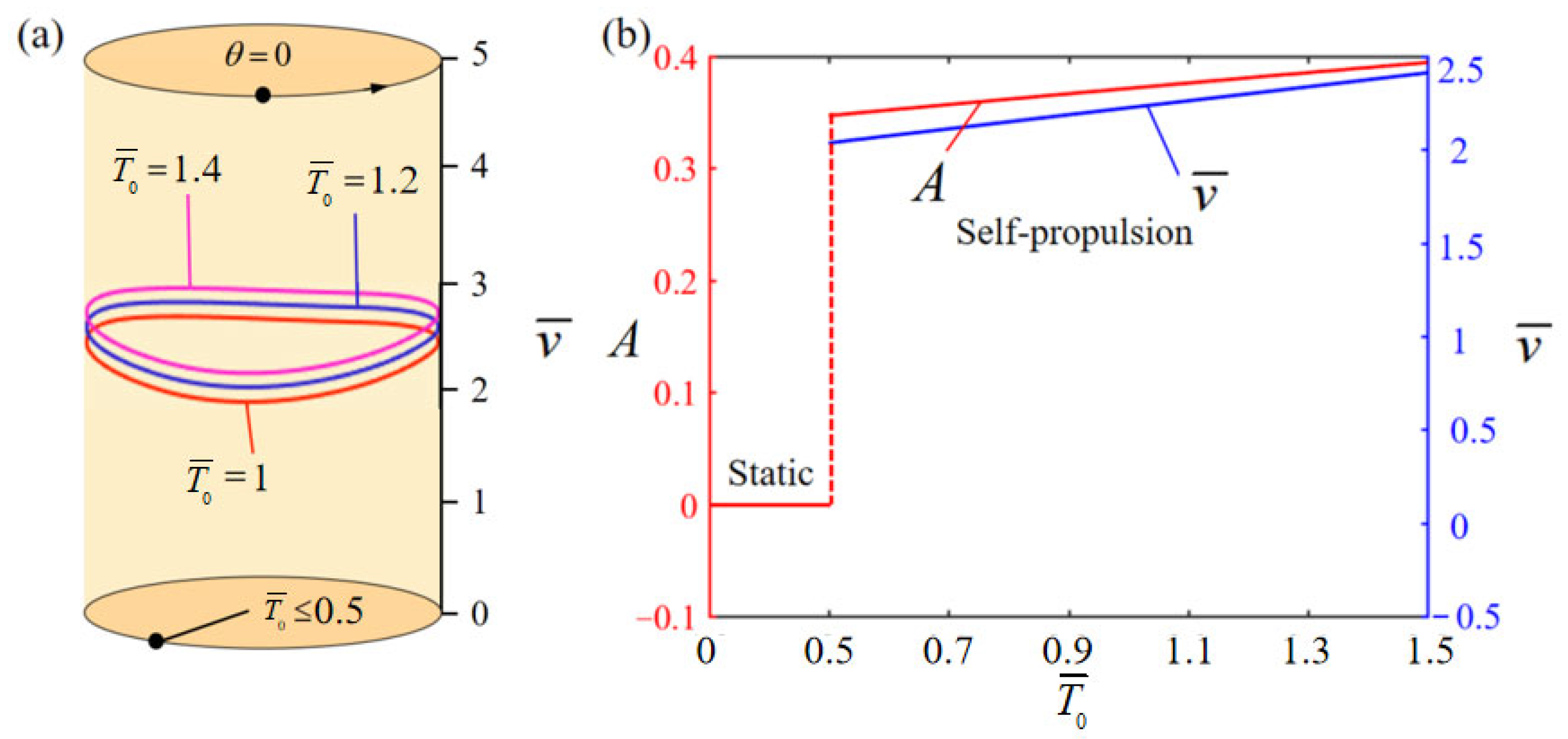
Figure 7 displays the impact of limit temperature on the self-propulsion of the system, in which the other parameters are , , , , , , , , , and . Figure 7a depicts the limit cycles for distinct limit temperature, highlighting that the critical limit temperature required for the system to initiate self-propulsion is approximately , and this is also consistent with the critical value calculated by Equation (21) in Figure 5. This critical value serves as the threshold for the system to enter the self-propulsion pattern, suggesting that the limit temperatures below this critical value are not sufficient to overcome the damping losses, causing the system to stabilize in static equilibrium. However, for limit temperatures of , and , the system exhibits the self-propulsion pattern. In addition, Figure 7b shows the effect of limit temperature on the self-propulsion speed of the system and the motion amplitude of the mass ball. As the limit temperature increases, the mass ball amplitude increases, leading to a faster self-propulsion speed of the system. This trend can be attributed to the fact that higher illumination intensity increases the production of thermal energy, thus improving the energy input.

Figure 7.
Effect of limit temperature on the self-propulsion of the system, with , , , , , , , , , and . (a) Limit cycles; (b) self-propulsion speed and mass ball amplitude.
4.3. Effect of Thermal Contraction Coefficient
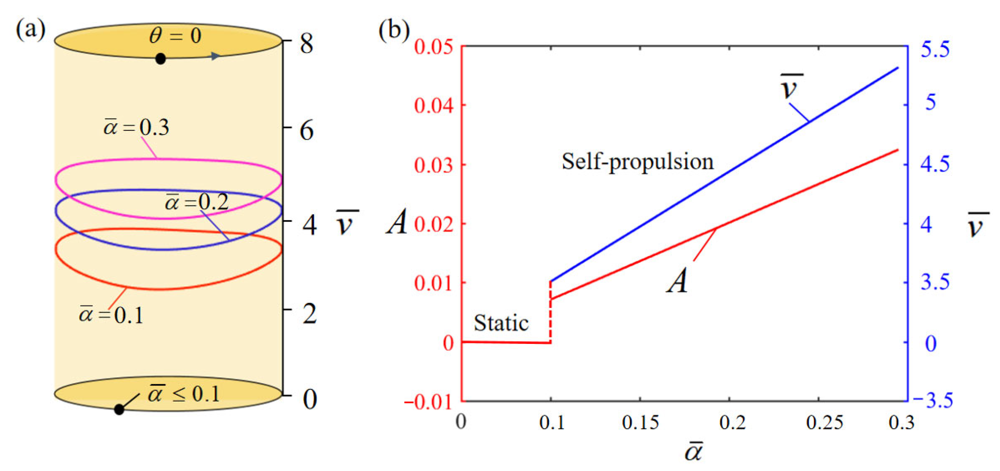
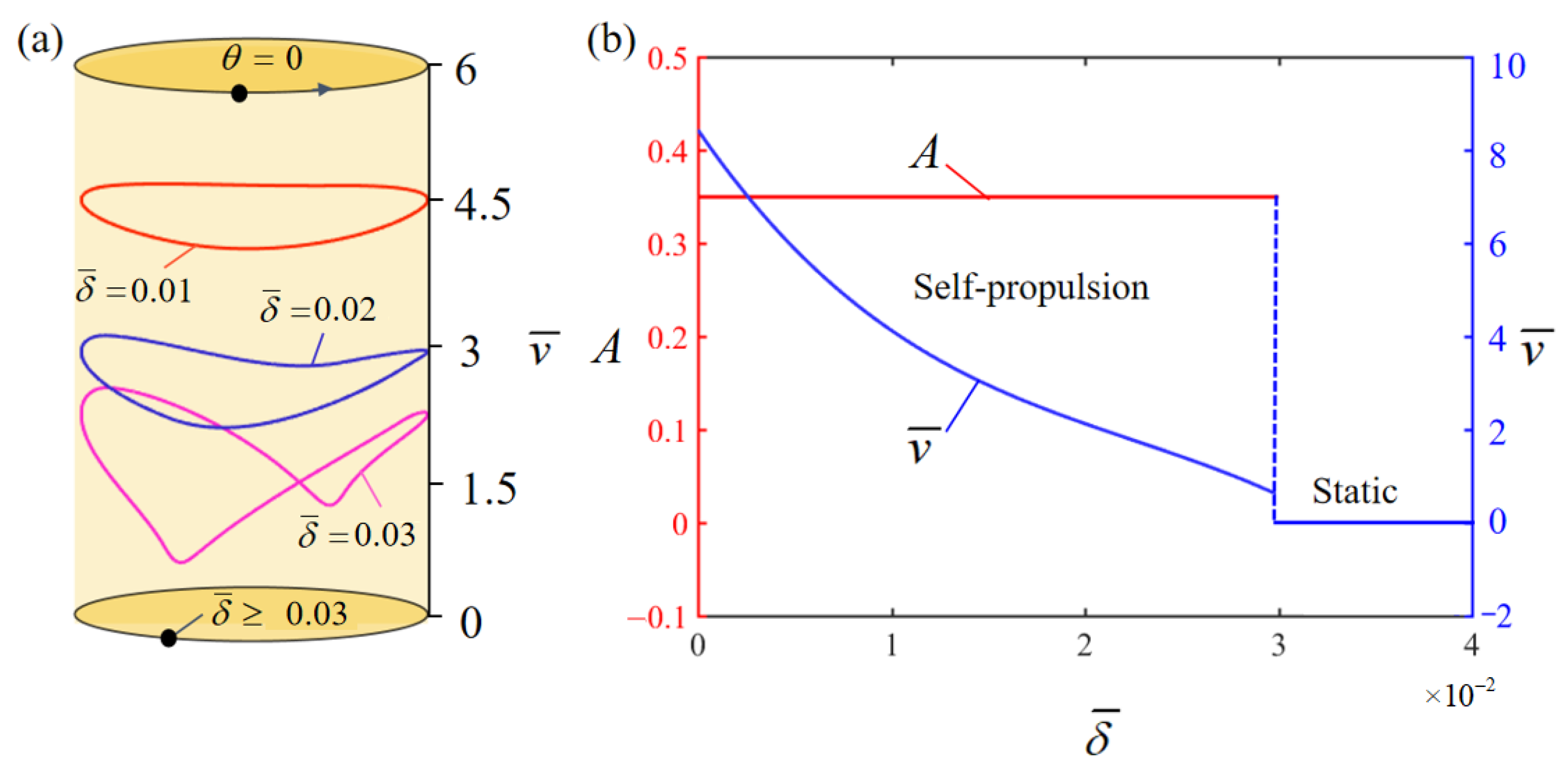
The effect of thermal contraction coefficient on the self-propulsion of the system is depicted in Figure 8. During the numerical analysis, other parameters are kept constant, namely, , , , , , , , , and . The limit cycles under different thermal contraction coefficients are plotted in Figure 8a. A critical value of the thermal contraction coefficient is present in the transition between self-propulsion and static patterns, i.e., , and this is also consistent with the critical value calculated by Equation (21) in Figure 5. For thermal contraction coefficients below this critical value, the energy input to the system is not sufficient to counteract the energy loss due to damping, leading to a steady static equilibrium. On the contrary, the system is in a self-propulsion pattern for thermal contraction coefficients of , and . Figure 8b demonstrates how thermal contraction coefficient affects the self-propulsion speed of the system and the motion amplitude of the mass ball. An increase in thermal contraction coefficient leads to an increase in both the self-propulsion speed and the mass ball amplitude. There exists a correlation between thermal contraction coefficient and the movement characteristics, i.e., an increase in the thermal contraction coefficient leads to a surge in an electrothermally driven contraction strain, which, in turn, corresponds to a rise in the amount of absorbed thermal energy. Therefore, an increase in the thermal contraction coefficient of the LCE material amplifies the efficiency of converting thermal energy into mechanical energy. This observation underscores the significance of the thermal contraction coefficient in the transition of the system from the static to self-propulsion pattern.

Figure 8.
Effect of thermal contraction coefficient on the self-propulsion of the system, with , , , , , , , , and . (a) Limit cycles; (b) self-propulsion speed and mass ball amplitude.
4.4. Effect of Turntable Radius
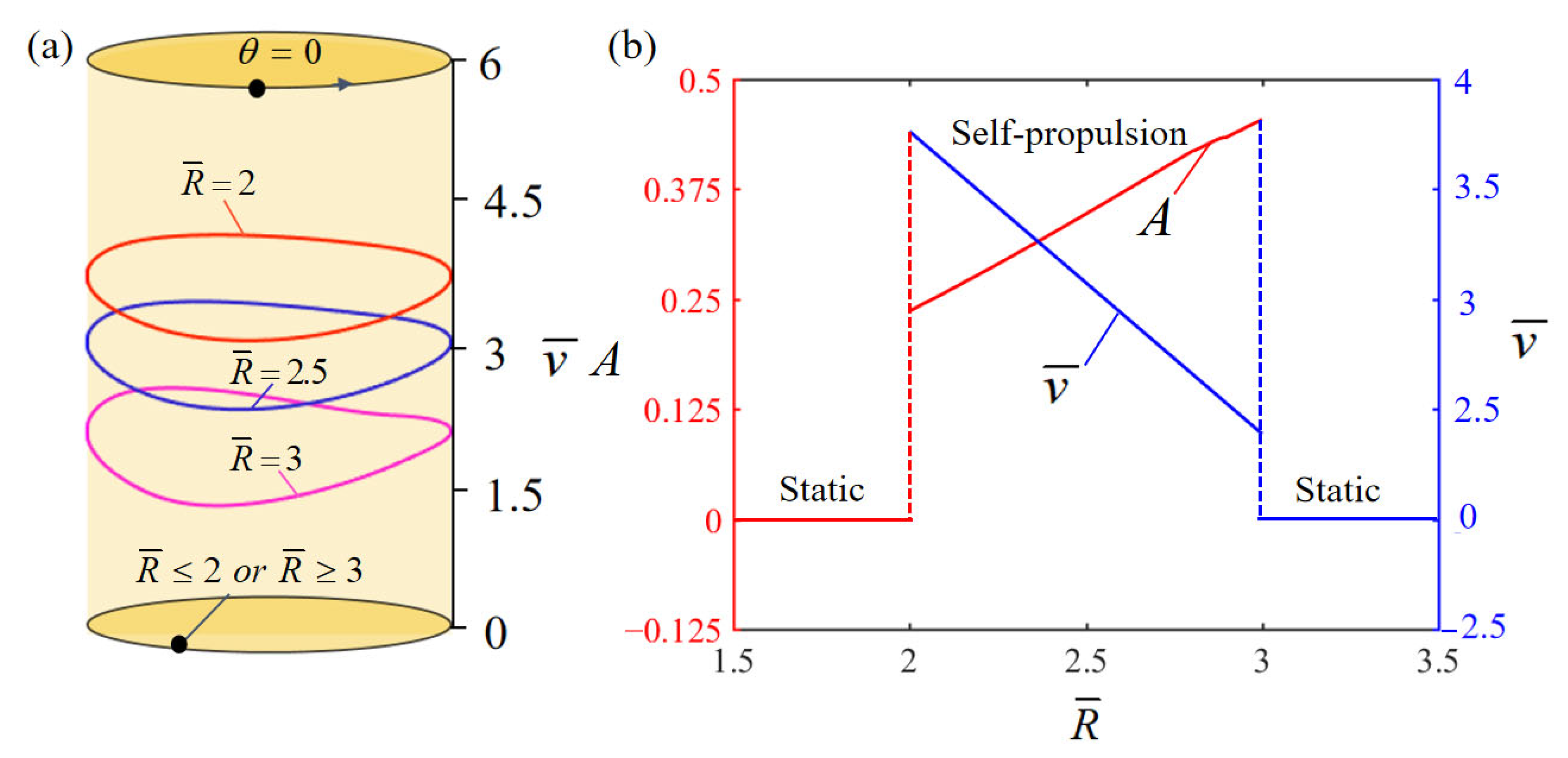
Figure 9 illustrates the effect of LCE turntable radius on the self-propulsion of the system, where the other parameters , , , , , , , , , and are held constant. Figure 9a plots the limit cycles for different turntable radii, showing the existence of a transition threshold between static and self-propulsion patterns, i.e., in the interval between 2 and 3, and this is also consistent with the critical value calculated by Equation (21). When the turntable radius is or , the energy conversion efficiency of the system is low, and the input mechanical energy is not enough to offset the energy loss from damping, which induces a static pattern. In contrast, at , , and , the system becomes a self-propulsion pattern. The effect of turntable radius on the self-propulsion speed and motion amplitude of the mass ball is displayed in Figure 9b. As the turntable radius increases, the self-propulsion speed of the automobile system decreases, whereas the motion amplitude of the mass ball rises. This correlation can be attributed to the fact that the small turntable radius provides insufficient mechanical energy to counteract the damping dissipation, coupled with the fact that the motion amplitude of the mass ball becomes larger as increases, leading to an increase in energy dissipation. Consequently, the system fails to maintain its self-propulsion due to insufficient mechanical energy generated.
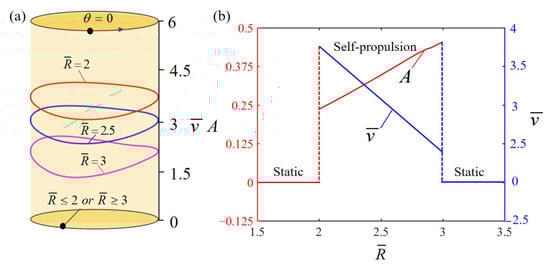
Figure 9.
Effect of LCE turntable radius on the self-propulsion of the system, with , , , , , , , , , and . (a) Limit cycles; (b) self-propulsion speed and mass ball amplitude.
4.5. Effect of Damping Factor
Figure 10 depicts the effect of damping factor on the self-propulsion of the system, while the other parameters are set to , , , , , , , , , and . Figure 10a draws the limit cycles corresponding to distinct damping factors, identifying a critical damping factor denoted as , which serves as the transition threshold between static and self-propulsion patterns, and this is also consistent with the critical value calculated by Equation (21). Above this critical value, the damping dissipation of the system becomes too pronounced to be compensated for by the mechanical energy generated by the input energy, thus stabilizing the automobile system in static equilibrium. Conversely, for , and , the self-propulsion pattern can be triggered. Figure 10b shows the effect of damping factor on the self-propulsion speed and the motion amplitude of the mass ball. The magnitude of the damping factor directly affects the energy dissipation, resulting in a reduction in the energy available for the rotation of the LCE turntable. As a result, the time of the rotational cycle of the LCE turntable increases, reflecting a decrease in the self-propulsion speed. It is important to note that the damping factor has a negligible effect on the amplitude of the mass ball.
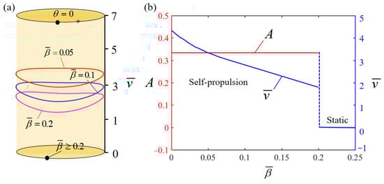
Figure 10.
Effect of damping factor on the self-propulsion of the system, with , , , , , , , , , and . (a) Limit cycles; (b) self-propulsion speed and mass ball amplitude.
4.6. Effect of Rolling Resistance Coefficient
The impact of rolling resistance coefficient on the self-propulsion of the system is presented in Figure 11. Firstly, Figure 11a displays the limit cycles for various rolling resistance coefficients, while Figure 11b plots the influence of rolling resistance coefficient on the self-propulsion speed and the motion amplitude of the mass ball. In the calculation, we chose specific values for other parameters such as , , , , , , , , , and . The critical value of the rolling resistance coefficient is approximately 0.03, and this is also consistent with the critical value calculated by Equation (21). When the rolling resistance coefficient does not exceed this value, the LCE turntable engine rotates and the automobile system can experience self-propulsion. Upon examining Figure 11b, we observe a gradual decrease in the self-propulsion speed as the rolling resistance coefficient increases, while the amplitude of the mass ball remains constant. This phenomenon can be attributed to the similarity between the rolling resistance coefficient and the damping factor in their effects on the system. Specifically, as the rolling resistance coefficient increases, there is greater damping dissipation, which ultimately leads to insufficient energy input from the external environment and eventually a static pattern.
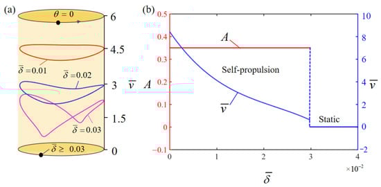
Figure 11.
Effect of rolling resistance coefficient on the self-propulsion of the system, with , , , , , , , , , and . (a) Limit cycles; (b) self-propulsion speed and mass ball amplitude.
4.7. Effect of Elastic Stiffness of LCE Rope
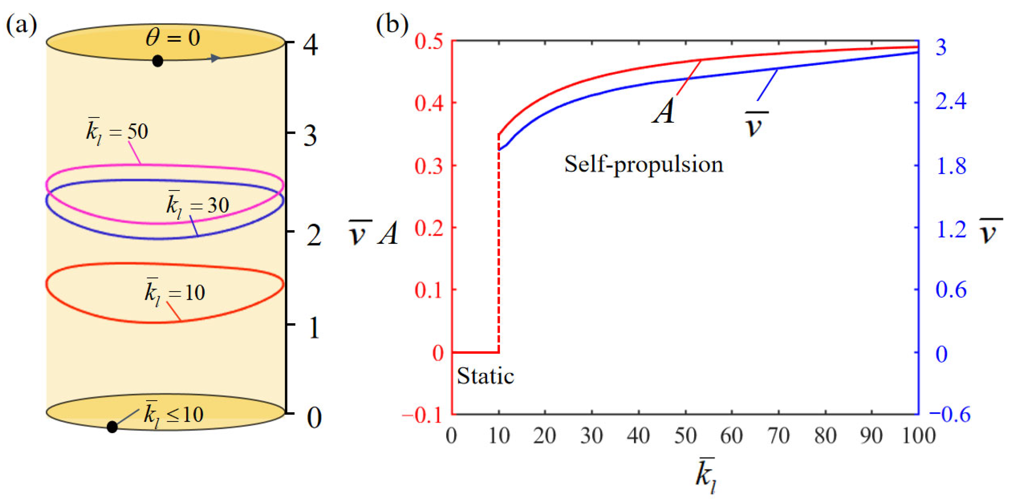
Figure 12a describes how the elastic stiffness of the LCE rope affects the self-propulsion of the system. The other parameters are chosen as , , , , , , , , , and . Figure 11a plots the limit cycles for different elastic stiffnesses of LCE rope. The critical value of the elastic stiffness of LCE rope is , which indicates the transition from the static pattern to the self-propulsion pattern, and this is also consistent with the critical value calculated by Equation (21). When the elastic stiffness falls below this critical value, the mechanical energy converted from heat is not sufficient to cover the energy dissipated through the damping effect, which results in a static pattern of the system. Instead, the system will undergo self-propulsion at , and . Figure 12b illustrates how the elastic stiffness of the LCE rope affects the self-propulsion speed and the motion amplitude of the mass ball. As the elastic stiffness of the LCE rope gradually increases, the self-propulsion speed and mass ball amplitude exhibit only slight increments. This is a consequence of the fact that the variation in the LCE rope is mainly dependent on the temperature variation, and its own elastic stiffness has a limited effect on the system.
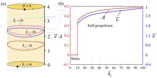
Figure 12.
Effect of elastic stiffness of LCE rope on the self-propulsion of the system, with , , , , , , , , , and . (a) Limit cycles; (b) self-propulsion speed and mass ball amplitude.
4.8. Effect of Elastic Stiffness of Spring
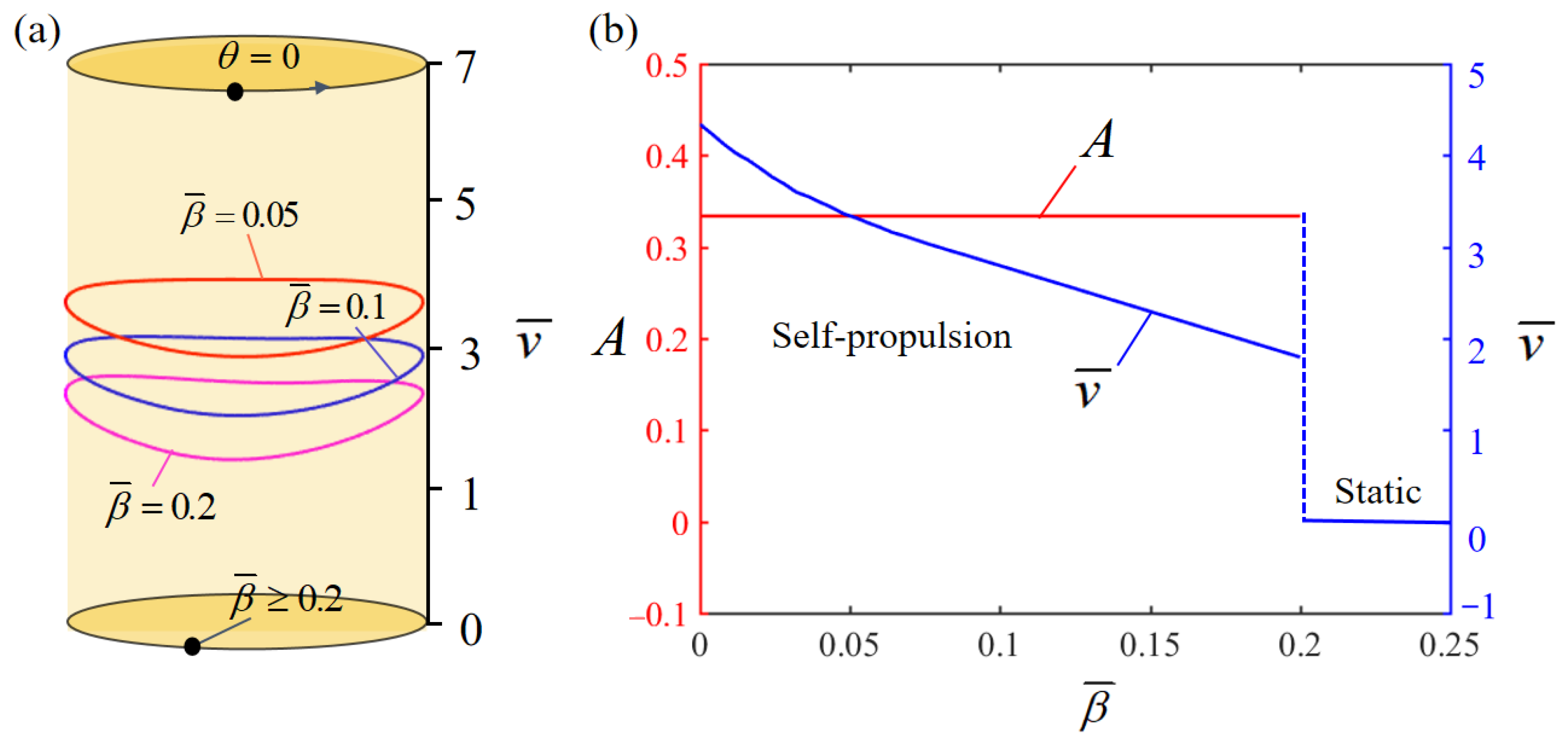
Figure 13 presents how the elastic stiffness of the spring influences the self-propulsion of the system, among which the other parameters are set as , , , , , , , , , and . Figure 13a plots the limit cycles under distinct elastic stiffnesses of spring. As observed, when the elastic stiffness of spring exceeds the critical value , the contraction time of the LCE rope in the illumination zone increases, leading to a reduction in the network generated by the driving torque. As a consequence, the network is not sufficient to compensate for the damping dissipation, resulting in the system eventually reaching a static equilibrium position, and this is also consistent with the critical value calculated by Equation (21). Figure 13b displays how the elastic stiffness of the spring affects the self-propulsion speed of the system and the amplitude of the mass ball. An increase in the elastic stiffness of the spring leads to a joint decrease in the self-propulsion speed and mass ball amplitude. This can be towing to the reduced displacement of the mass ball in the illumination zone, resulting from the increased elastic stiffness of spring. Consequently, this reduction in displacement leads to a lower efficiency in the conversion of thermal energy into mechanical energy, ultimately resulting in a decrease in the self-propulsion speed of the system and amplitude of the mass ball within the system.
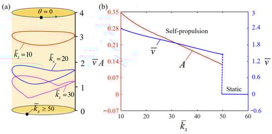
Figure 13.
Effect of elastic stiffness of spring on the self-propulsion of the system, with , , , , , , , , , and . (a) Limit cycles; (b) self-propulsion speed and mass ball amplitude.
4.9. Effect of Illumination Zone Angle
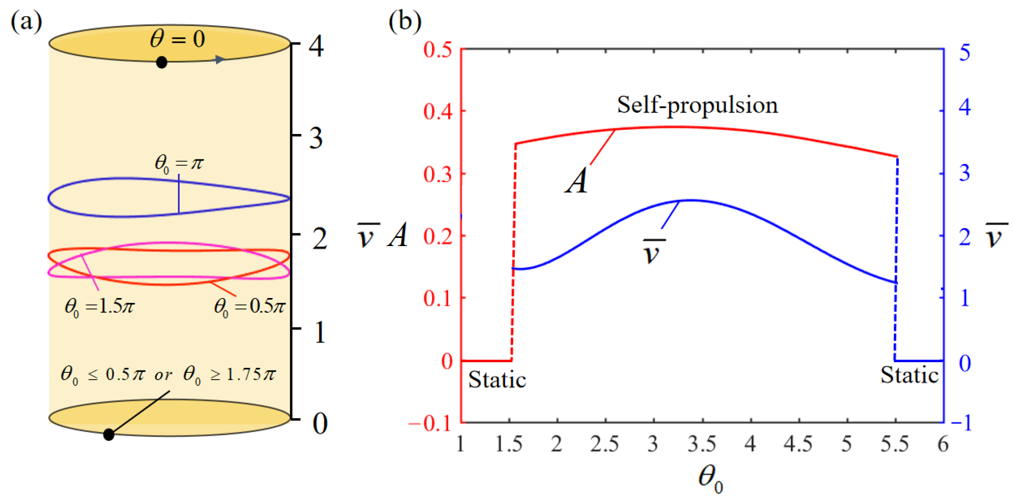
The effect of illumination zone angle on the self-propulsion of the system is depicted in Figure 14, with other parameters being , , , , , , , , , and . The limit cycles under distinct illumination zone angles are drawn in Figure 14a, identifying two critical illumination zone angles, approximately and , which delineate the transition from static to self-propulsion pattern. When the illumination zone angle is below the critical threshold , the LCE rope is not exposed to the illumination zone long enough, resulting in insufficient energy input to offset the energy loss due to the damping effect, and thus the system remains in static equilibrium. On the contrary, when the illumination zone angle exceeds , the LCE rope is exposed to the dark zone for too short a period of time to restore it to its initial state, leading to the thermal energy supplied to the system being unable to offset the damping dissipation, which ultimately results in the static equilibrium of the system. However, for illumination zone angles within the range of and , the system can initiate self-propulsion. The effect of illumination zone angle on the self-propulsion speed of the system and the motion amplitude of the mass ball is illustrated in Figure 14b. Apparently, with the increase in the illumination zone angle, both the self-propulsion speed and the mass ball amplitude tend to first increase and then decrease. This is similar to the reasons mentioned above that too small or too large an illumination zone can negatively affect the system.
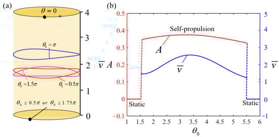
Figure 14.
Effect of illumination zone angle on the self-propulsion of the system, with , , , , , , , , , and . (a) Limit cycles; (b) self-propulsion speed and mass ball amplitude.
In summary, this section systematically sorts out the effects of various key dimensionless system parameters on the self-propulsion speed of the system as well as the amplitude A of the mass ball in the LCE turntable, which are summarized in Table 3. The presented data provide indispensable insights into the engineering design of self-excited motion systems, enabling precise control of self-excited motion attributes in practical applications.
Table 3.
Effects of several key dimensionless parameters.
5. Conclusions
Characterized by the ability to absorb energy from stable environments and self-regulate, self-excited motion shows significant potential for microdevices, autonomous robotics, sensor technology and energy generation. In the current paper, an LCE turntable-engined automobile system capable of self-propulsion under steady illumination is investigated. A nonlinear theoretical model is proposed, which is combined with an established photothermally responsive LCE model, and the dynamic behavior of the automobile system under steady illumination is analyzed with data via the fourth-order Runge–Kutta method. Numerical calculations suggest that two different motion patterns occur in the automobile system under steady illumination: static pattern and self-propulsion pattern. The correlation between thermal energy and damping dissipation is crucial to maintain the motion of the system. This paper also provides insight into the critical conditions for initiating self-propulsion and investigates the effect of key system parameters on the self-excited motion of the system. The key parameters affecting self-propulsion include gravitational acceleration, LCE turntable radius, elastic stiffnesses of the LCE rope and spring, limit temperature, illumination zone angle, thermal contraction coefficient, damping factor, and roll resistance coefficient. These parameters also determine the self-propulsion speed of the system and the motion amplitude of the mass ball in the LCE turntable. The proposed system with zero-energy mode motions has the advantage of simple structural design, easy control, low friction and stable kinematics. The findings provide innovative design perspectives for self-propulsion systems, enhancing our comprehension of their underlying principles and its versatile applications in energy harvesting, monitoring, soft robotics, and micro- and nano-devices.
Certainly, there are some limitations of the system. For example, the energy conversion efficiency of photothermal LCE primarily depends on the light absorption and conversion mechanism. The low photothermal conversion efficiency of current materials restricts their practical applications. Once light energy is converted into thermal energy, deformation is driven by thermal expansion or phase change, leading to significant energy loss in the process. Additionally, the response rate of photothermal LCE is constrained by the thermal diffusivity and thermal conductivity properties of the material. Meanwhile, the stability of natural light sources may be insufficient for its potential energy resources and possible applications. Conversely, the use of artificial light sources could potentially increase overall energy consumption. Furthermore, applications in high-precision fields require more complex control systems and improved energy conversion efficiency, leading to significantly higher costs. Despite these limitations, this study provides important initial insights into the relevant field and lays the groundwork for further research in the future.
Author Contributions
Conceptualization, K.L.; Methodology, Z.Y.; Software, Z.Y.; Validation, Y.D.; Writing—original draft, Z.Y.; Writing—review & editing, Y.D., J.L. and K.L.; Supervision, J.L. All authors have read and agreed to the published version of the manuscript.
Funding
This study is supported by National Natural Science Foundation of China (No. 12172001), University Natural Science Research Project of Anhui Province (Nos. 2022AH030035, 2022AH020029 and KJ2021ZD0066), Outstanding Talents Cultivation Project of Universities in Anhui (No. gxyq2022029), Anhui Provincial Natural Science Foundation (Nos. 2208085Y01 and 2008085QA23) and Housing and Urban-Rural Development Science and Technology Project of Anhui Province (No. 2023-YF129).
Data Availability Statement
The original contributions presented in the study are included in the article, further inquiries can be directed to the corresponding author.
Conflicts of Interest
The authors declare no conflict of interest.
References
- Ding, W.J. Self-Excited Vibration; Tsing–Hua University Press: Beijing, China, 2009. [Google Scholar]
- Liu, Z.; Qi, M.; Zhu, Y.; Huang, D.; Zhang, X.; Lin, L.; Yan, X. Mechanical response of the isolated cantilever with a floating potential in steady electrostatic field. Int. J. Mech. Sci. 2019, 161, 105066. [Google Scholar] [CrossRef]
- Charroyer, L.; Chiello, O.; Sinou, J.J. Self−excited vibrations of a nonsmooth contact dynamical system with planar friction based on the shooting method. Int. J. Mech. Sci. 2018, 144, 90–101. [Google Scholar] [CrossRef]
- Hu, W.; Lum, G.Z.; Mastrangeli, M.; Sitti, M. Small−scale soft−bodied robot with multimodal locomotion. Nature 2018, 554, 81–85. [Google Scholar] [CrossRef] [PubMed]
- Iliuk, I.; Balthazar, J.M.; Tusset, A.M.; Piqueira, J.R.; Pontes, D.B.R.; Felix, J.L.; Bueno, A.M. Application of passive control to energy harvester efficiency using a nonideal portal frame structural support system. J. Intell. Mater. Syst. Struct. 2014, 25, 417–429. [Google Scholar] [CrossRef]
- Korner, K.; Kuenstler, A.S.; Hayward, R.C.; Audoly, B.; Bhattacharya, K. A nonlinear beam model of photomotile structures. Proc. Natl. Acad. Sci. USA 2020, 117, 9762–9770. [Google Scholar] [CrossRef] [PubMed]
- Martella, D.; Nocentini, S.C.; Parmeggiani, C.; Wiersma, D.S. Self−regulating capabilities in photonic robotics. Adv. Mater. Technol. 2019, 4, 1800571. [Google Scholar] [CrossRef]
- Sangwan, V.; Taneja, A.; Mukherjee, S. Design of a robust self−excited biped walking mechanism. Mech. Theory 2004, 39, 1385–1397. [Google Scholar] [CrossRef]
- Erturk, A.; Inman, D.J. Piezoelectric Energy Harvesting; John Wiley & Sons: Hoboken, NJ, USA, 2011. [Google Scholar]
- Rosso, M. Intentional and Inherent Nonlinearities in Piezoelectric Energy Harvesting; Springer Nature: Berlin/Heidelberg, Germany, 2024. [Google Scholar]
- Briand, D.; Yeatman, E.; Roundy, S. Micro Energy Harvesting; John Wiley & Sons: Hoboken, NJ, USA, 2015; ISBN 978-3-527-31902-2. [Google Scholar]
- Mohsen, S.; Henry, A.S.; Steven, R.A. A review of energy harvesting using piezoelectric materials: State-of-the-art a decade later (2008–2018). Smart Mater. Struct. 2019, 28, 113001. [Google Scholar]
- Lin, Y.-L.; Kyung, C.-M.; Hiroto, Y.; Liu, Y. Smart Sensors and Systems; Springer Nature Switzerland AG: Cham, Switzerland, 2020. [Google Scholar]
- Ambaye, G.; Boldsaikhan, E.; Krishnan, K. Soft Robot Design, Manufacturing, and Operation Challenges: A Review. J. Manuf. Mater. Process. 2024, 8, 79. [Google Scholar] [CrossRef]
- Yang, Z. Advanced MEMS/NEMS Fabrication and Sensors; Springer: Berlin/Heidelberg, Germany, 2022. [Google Scholar]
- Alberto, C.; Raffaele, A.; Claudia, C.; Attilio, F.; Aldo, G. Stefano Mariani, Mechanics of Microsystems; Wiley: Hoboken, NJ, USA, 2018; ISBN 9781119053835. [Google Scholar]
- Yoshida, R. Self−oscillating gels driven by the Belousov−Zhabotinsky reaction as novel smart materials. Adv. Mater. 2010, 22, 3463–3483. [Google Scholar] [CrossRef]
- Yashin, V.V.; Balazs, A.C. Pattern formation and shape changes in self−oscillating polymer gels. Science 2006, 314, 798–801. [Google Scholar] [CrossRef]
- Boissonade, J.; Kepper, P.D. Multiple types of spatio−temporal oscillations induced by differential diffusion in the Landolt reaction. Phys. Chem. Chem. Phys. 2011, 13, 4132–4137. [Google Scholar] [CrossRef] [PubMed]
- He, Q.G.; Wang, Z.J.; Wang, Y.; Wang, Z.J.; Li, C.H.; Annapooranan, R.; Zeng, J.; Chen, R.K.; Cai, S. Electrospun liquid crystal elastomer microfiber actuator. Sci. Robot. 2021, 6, eabi9704. [Google Scholar] [CrossRef] [PubMed]
- Yang, H.; Zhang, C.; Chen, B.; Wang, Z.; Xu, Y.; Xiao, R. Bioinspired design of stimuli-responsive artificial muscles with multiple actuation modes. Smart Mater. Struct. 2023, 32, 085023. [Google Scholar] [CrossRef]
- Park, S.; Oh, Y.; Moon, J.; Chung, H. Recent Trends in Continuum Modeling of Liquid Crystal Networks: A Mini−Review. Polymers 2023, 15, 1904. [Google Scholar] [CrossRef]
- Hu, Z.; Li, Y.; Lv, J. Phototunable self−oscillating system driven by a self−winding fiber actuator. Nat. Commun. 2021, 12, 3211. [Google Scholar] [CrossRef] [PubMed]
- Zhao, Y.; Chi, Y.; Hong, Y.; Li, Y.; Yang, S.; Yin, J. Twisting for soft intelligent autonomous robot in unstructured environments. Proc. Natl. Acad. Sci. USA 2022, 119, e2200265119. [Google Scholar] [CrossRef] [PubMed]
- Graeber, G.; Regulagadda, K.; Hodel, P.; Küttel, C.; Landolf, D.; Schutzius, T.; Poulikakos, D. Leidenfrost droplet trampolining. Nat. Commun. 2021, 12, 1727. [Google Scholar] [CrossRef]
- Chakrabarti, A.; Choi, G.P.T.; Mahadevan, L. Self−Excited Motions of Volatile Drops on Swellable Sheets. Phys. Rev. Lett. 2020, 124, 258002. [Google Scholar] [CrossRef]
- Lv, X.; Yu, M.; Wang, W.; Yu, H. Photothermal pneumatic wheel with high loadbearing capacity. Compos. Commun. 2021, 24, 100651. [Google Scholar] [CrossRef]
- Tang, R.; Liu, Z.; Xu, D.; Liu, J.; Yu, L.; Yu, H. Optical pendulum generator based on photomechanical liquid−crystalline actuators. ACS Appl. Mater. Interfaces 2015, 7, 8393–8397. [Google Scholar] [CrossRef] [PubMed]
- Wu, H.; Lou, J.; Zhang, B.; Dai, Y.; Li, K. Stability analysis of a liquid crystal elastomer self-oscillator under a linear temperature field. Appl. Math. Mech. (Engl. Ed.) 2024, 45, 337–354. [Google Scholar] [CrossRef]
- Lahikainen, M.; Zeng, H.; Priimagi, A. Reconfigurable photoactuator through synergistic use of photochemical and photo thermal effects. Nat. Commun. 2018, 9, 4148. [Google Scholar] [CrossRef]
- Kim, Y.; Berg, J.; Crosby, A.J. Autonomous snapping and jumping polymer gels. Nat. Mater. 2021, 20, 1695–1701. [Google Scholar] [CrossRef] [PubMed]
- Wu, H.; Dai, Y.; Li, K.; Xu, P. Theoretical study of chaotic jumping of liquid crystal elastomer ball under periodic illumination. Nonlinear Dyn. 2024, 112, 5349–5360. [Google Scholar] [CrossRef]
- Xu, P.; Chen, Y.; Wu, H.; Dai, Y.; Li, K. Chaotic motion behaviors of liquid crystal elastomer pendulum under periodic illumination. Results Phys. 2024, 56, 107332. [Google Scholar] [CrossRef]
- Liu, J.; Shi, F.; Song, W.; Dai, Y.; Li, K. Modeling of self-oscillating flexible circuits based on liquid crystal elastomers. Int. J. Mech. Sci. 2024, 270, 109099. [Google Scholar] [CrossRef]
- Wu, H.; Zhao, C.; Dai, Y.; Li, K. Light-fueled self-fluttering aircraft with a liquid crystal elastomer-based engine. Commun. Nonlinear Sci. Numer. Simul. 2024, 133, 107942. [Google Scholar] [CrossRef]
- Yu, Y.; Hu, H.; Dai, Y.; Li, K. Modeling the light-powered self-rotation of a liquid crystal elastomer fiber-based engine. Phys. Rev. E 2024, 109, 034701. [Google Scholar] [CrossRef]
- Wu, H.; Zhao, C.; Dai, Y.; Li, K. Modeling of a light-fueled self-paddling boat with a liquid crystal elastomer-based motor. Phys. Rev. E 2024, 109, 044705. [Google Scholar] [CrossRef]
- Qiu, Y.; Chen, J.; Dai, Y.; Zhou, L.; Yu, Y.; Li, K. Mathematical Modeling of the Displacement of a Light-Fuel Self-Moving Automobile with an On-Board Liquid Crystal Elastomer Propulsion Device. Mathematics 2024, 12, 1322. [Google Scholar] [CrossRef]
- Cunha, M.; Peeketi, A.R.; Ramgopal, A.; Annabattula, R.K.; Schenning, A. Light−driven continual oscillatory rocking of a polymer film. Chem. Open 2020, 9, 1149–1152. [Google Scholar]
- Cheng, Y.; Lu, H.; Lee, X.; Zeng, H.; Priimagi, A. Kirigami−based light−induced shape−morphing and locomotion. Adv. Mater. 2019, 32, 1906233. [Google Scholar] [CrossRef]
- Gelebart, A.H.; Mulder, D.J.; Varga, M.; Konya, A.; Vantomme, G.; Meijer, E.W.; Selinger, R.S.; Broer, D.J. Making waves in a photoactive polymer film. Nature 2017, 546, 632–636. [Google Scholar] [CrossRef] [PubMed]
- Warner, M.; Terentjev, E.M. Liquid Crystal Elastomers; Oxford University Press: London, UK, 2007. [Google Scholar]
- Corbett, D.; Warner, M. Linear and nonlinear photoinduced deformations of can−tilevers. Phys. Rev. Lett. 2007, 99, 174302. [Google Scholar] [CrossRef] [PubMed]
- Qiu, Y.; Wu, H.; Dai, Y.; Li, K. Behavior prediction and inverse design for self-rotating skipping ropes based on random forest and neural network. Mathematics 2024, 12, 1019. [Google Scholar] [CrossRef]
- Wu, H.; Zhang, B.; Li, K. Synchronous behaviors of three coupled liquid crystal elastomer-based spring oscillators under linear temperature fields. Phys. Rev. E 2024, 109, 024701. [Google Scholar] [CrossRef]
- Wu, H.; Lou, J.; Dai, Y.; Zhang, B.; Li, K. Bifurcation analysis in liquid crystal elastomer spring self-oscillators under linear light fields. Chaos Solitons Fractals 2024, 181, 114587. [Google Scholar] [CrossRef]
- Chen, B.; Liu, C.; Xu, Z.; Wang, Z.; Xiao, R. Modeling the thermo-responsive behaviors of polydomain and monodomain nematic liquid crystal elastomers. Mech. Mater. 2024, 188, 104838. [Google Scholar] [CrossRef]
- Bisoyi, H.K.; Urbas, A.M.; Li, Q. Soft materials driven by photo thermal effect and their applications. Adv. Opt. Mater. 2018, 6, 1800458. [Google Scholar] [CrossRef]
- Yu, Y.; Li, L.; Liu, E.; Han, X.; Wang, J.; Xie, Y.; Lu, C. Light−driven core−shell fiber actuator based on carbon nanotubes/liquid crystal elastomer for artificial muscle and phototropic locomotion. Carbon 2022, 187, 97–107. [Google Scholar] [CrossRef]
- Sun, J.; Wang, Y.; Liao, W.; Yang, Z. Ultrafast, High-Contractile Electrothermal-Driven Liquid Crystal Elastomer Fibers towards Artificial Muscles. Small 2021, 17, 2103700. [Google Scholar] [CrossRef] [PubMed]
- Lu, D.; Wang, L.; Chen, B.; Xu, Z.; Wang, Z.; Xiao, R. Shape memory behaviors of 3D printed liquid crystal elastomers. Soft Sci. 2023, 3, 4. [Google Scholar]
- Wang, L.; Wei, Z.; Xu, Z.; Yu, Q.; Wu, Z.L.; Wang, Z.; Qian, J.; Xiao, R. Shape Morphing of 3D Printed Liquid Crystal Elastomer Structures with Precuts. ACS Appl. Polym. Mater. 2023, 5, 7477–7484. [Google Scholar] [CrossRef]
- Wang, Y.; Yin, R.; Jin, L.; Liu, M.; Gao, Y.; Raney, J.; Yang, S. 3D-Printed Photoresponsive Liquid Crystal Elastomer Composites for Free-Form Actuation. Adv. Funct. Mater. 2023, 33, 2210614. [Google Scholar] [CrossRef]
- He, Q.; Wang, Z.; Wang, Y.; Minori, A.; Tolley, M.T.; Cai, S. Electrically controlled liquid crystal elastomer–based soft tubular actuator with multimodal actuation. Sci. Adv. 2019, 5, eaax5746. [Google Scholar] [CrossRef] [PubMed]
- Liao, B.; Zang, H.; Chen, M.; Wang, Y.; Lang, X.; Zhu, N.; Yang, Z.; Yi, Y. Soft rod−climbing robot inspired by winding locomotion of snake. Soft Robot. 2020, 7, 500–511. [Google Scholar] [CrossRef] [PubMed]
- Haberl, J.M.; Sanchez-Ferrer, A.; Mihut, A.M.; Dietsch, H.; Hirt, A.M.; Mezzenga, R. Liquid−crystalline elastomer−nanoparticle hybrids with reversible switch of magnetic memory. Adv. Mater. 2013, 25, 1787–1791. [Google Scholar] [CrossRef]
- Li, M.H.; Keller, P.; Li, B.; Wang, X.; Brunet, M. Light−driven side−on nematic elastomer actuators. Adv. Mater. 2003, 15, 569–572. [Google Scholar] [CrossRef]
- Qian, X.; Chen, Q.; Yang, Y.; Xu, Y.; Li, Z.; Wang, Z.; Wu, Y.; Wei, Y.; Ji, Y. Untethered recyclable tubular actuators with versatile locomotion for soft continuum robots. Adv. Mater. 2018, 30, 1801103. [Google Scholar] [CrossRef]
- Wei, Z.; Tianle, S.; Yuntong, D.; Kai, L.; Zhao, J. Light-powered self-propelled trolley with a liquid crystal elastomer pendulum motor. Int. J. Solids Struct. 2023, 285, 112500. [Google Scholar]
- Strogatz, S.H. Nonlinear Dynamics and Chaos: With Applications to Physics, Biology, Chemistry, and Engineering; CRC Press: Boca Raton, FL, USA, 2018. [Google Scholar]
- Pacejka, H. Tire and Vehicle Dynamics; Elsevier: Amsterdam, The Netherlands, 2005. [Google Scholar]
- Atanackovic, T.M.; Guran, A. Hooke’s law. In Theory of Elasticity for Scientists and Engineers; Springer: Berlin/Heidelberg, Germany, 2000; pp. 85–111. [Google Scholar]
- Camacho-Lopez, M.; Finkelmann, H.; Palffy-Muhoray, P.; Shelley, M. Fast liquid-crystal elastomer swims into the dark. Nat. Mater. 2004, 3, 307. [Google Scholar] [CrossRef] [PubMed]
- Hogan, P.M.; Tajbakhsh, A.R.; Terentjev, E.M. UV manipulation of order and macroscopic shape in nematic elastomers. Phys. Rev. 2002, 65, 041720. [Google Scholar] [CrossRef] [PubMed]
- Baumann, A.; Sánchez-Ferrer, A.; Jacomine, L.; Martinoty, P.; Houerou, V.; Ziebert, F.; Kulić, I. Motorizing fibers with geometric zero-energy modes. Nat. Mater. 2018, 17, 523. [Google Scholar] [CrossRef] [PubMed]

Disclaimer/Publisher’s Note: The statements, opinions and data contained in all publications are solely those of the individual author(s) and contributor(s) and not of MDPI and/or the editor(s). MDPI and/or the editor(s) disclaim responsibility for any injury to people or property resulting from any ideas, methods, instructions or products referred to in the content. |
© 2024 by the authors. Licensee MDPI, Basel, Switzerland. This article is an open access article distributed under the terms and conditions of the Creative Commons Attribution (CC BY) license (https://creativecommons.org/licenses/by/4.0/).