Abstract
With its formidable nonlinear mapping capabilities, deep learning has been widely applied in bearing remaining useful life (RUL) prediction. Given that equipment in actual work is subject to numerous disturbances, the collected data tends to exhibit random missing values. Furthermore, due to the dynamic nature of wind turbine environments, LSTM models relying on manually set parameters exhibit certain limitations. Considering these factors can lead to issues with the accuracy of predictive models when forecasting the remaining useful life (RUL) of wind turbine bearings. In light of this issue, a novel strategy for predicting the remaining life of wind turbine bearings under data scarcity conditions is proposed. Firstly, the average similarity (AS) is introduced to reconstruct the discriminator of the Generative Adversarial Imputation Nets (GAIN), and the adversarial process between the generative module and the discriminant is strengthened. Based on this, the dung beetle algorithm (DBO) is used to optimize multiple parameters of the long-term and short-term memory network (LSTM), and the complete data after filling is used as the input data of the optimized LSTM to realize the prediction of the remaining life of the wind power bearing. The effectiveness of the proposed method is verified by the full-life data test of bearings. The results show that, under the condition of missing data, the new strategy of AS-GAIN-LSTM is used to predict the RUL of wind turbine bearings, which has a more stable prediction performance.
MSC:
68T07
1. Introduction
Wind power is a crucial area of development in the modern world, with wind turbines serving as the primary means of harnessing this renewable energy source [1]. Among the core components of wind turbines, wind turbine bearings play a pivotal role in their operation. However, they are vulnerable to various failure modes due to environmental uncertainties and other factors, which can negatively impact the stability and safety of the turbine equipment. In severe cases, this may result in irreparable financial losses and personnel casualties [2]. Therefore, there is an urgent need and significant importance in conducting predictive maintenance research based on real-time wind turbine bearing monitoring data.
Currently, there are three types of methods for predicting the remaining life of rolling bearings: those based on failure mechanism models [3,4], those based on statistical models [5,6], and those based on machine-learning techniques [7,8,9]. Among these, methods based on failure mechanism models may have difficulty describing the damage mechanisms of complex mechanical systems. Statistical models may not be able to capture nonlinear information, which makes it challenging to match the current complex and variable operating conditions. Most machine-learning approaches cannot deeply analyze and process state signals [10].
Due to its adaptability to diverse and complex scenarios, deep learning [11] has been extensively applied in the field of predicting the remaining life of bearings. Based on a Recursive Neural Network (RNN), Guo et al. [12] constructed a comprehensive health index RNN-HI considering the monotonicity and correlation of features, which solved the problem that the fault threshold was challenging to determine. They completed the RUL prediction of wind turbine generator bearings through a particle filter algorithm. Chen et al. [13] proposed a model based on the combination of RNN and autoencoder that realized the intelligent extraction of features, the construction of a complete end-to-end model of health indicators, and life prediction. Xiang et al. [14] proposed a lightweight regression operator based on RNN to balance the accuracy and simplicity of the model. Finally, the RUL prediction of aero-engine bearings was realized by using the deep learning framework model based on RNN.
Considering the correlation between bearing degradation process and time, Long Short-Term Memory (LSTM) has been favored by researchers because of its powerful time series processing ability [15]. Li et al. [16] used the Gorilla Troops Optimizer (GTO) to improve the prediction performance of the combined model of the Convolutional Neural Network (CNN) and LSTM. The vibration signal of the bearing was transformed into a frequency domain amplitude signal. The CNN was used to automatically extract feature information, and the deep features were introduced into the LSTM to predict the bearing RUL. Combining the advantages of LSTM and statistical process analysis, Liu et al. [17] proposed a LSS prediction model. Firstly, the time characteristics of aero-engine bearing vibration signals are extracted by statistical process analysis. Then, the multi-stage signals are input into LSS to complete the prediction of RUL. In order to enhance the model’s ability to learn features, L. Magadá et al. [18] proposed a combined model of Stacked Variational Denoising Autoencoder (SVDAE) to construct health indicators and Bidirectional Long Short-Term Memory (Bi-LSTM) for bearing RUL prediction. The experimental results show that the model has relatively stable performance. The parameters of LSTM typically consist of those in the input layer, hidden layer, output layer, and memory cells. These parameters play a crucial role in the training process of deep learning models. By adjusting these parameters, one can influence the model’s performance, prediction accuracy, and generalization capacity. Li et al. [19] proposed a predictive model based on Bayesian optimization (BO), Spatial-Temporal Attention (STA), and LSTM. This model adjusts the parameters of the LSTM through Bayesian optimization and applies it to building energy consumption prediction. Results showed that Bayesian optimization alone improved the model’s performance by 0.0717. Li et al. [20] used the Peafowl Optimization Algorithm (POA) to optimize the parameters of LSTM and built a POA-LSTM regression prediction model. Through experimental verification, the optimized model demonstrated higher accuracy.
At present, the construction of RUL prediction models is mostly based on the assumption that data acquisition is normal and that data is continuous and uniform. However, at the data acquisition site, due to operator errors, sensor failures, etc. [21], data loss or an uneven data interval may occur in the same equipment data acquisition cycle. Scholars have proposed some feasible data filling methods in terms of missing data. Rădulescu et al. [22] proposed the mean imputation model, which is a statistical method used for data interpolation. For numerical type data, the missing part of the column is interpolated by the average of all the existing values in the missing attribute column, so that the missing sequence becomes a complete sequence. Yang et al. [23] proposed a regression interpolation method. Firstly, a regression model is constructed based on the degree of correlation between different attribute elements. Then, the specific parameters of the constructed model are obtained according to the complete sample records in the data set. Finally, the missing values are filled by the model. Han et al. [24] used weighted K-Nearest Neighbor (KNN) to obtain globally similar instances and capture fluctuations in local regions, completed the filling of missing values under the two-cycle mechanism related to the ranking of missing variables and missing instances, and obtained better filling results on the sewage treatment plant dataset. Liu et al. [25] proposed an incomplete data filling method based on perceptual CNN, which was successfully applied to the prediction of power generation and improved the prediction performance. Wind turbines are usually installed in areas with large amounts of dust, severe sunshine, or high humidity. The working environment is very harsh, and the load range, temperature, and humidity are large [26], which makes it more prone to data loss. However, the above missing value filling method still needs to be improved when dealing with a complex data with high missing rate.
Based on this, a residual life prediction method for wind power bearing based on deep learning is proposed under the condition that data is missing. Aiming at the problem of missing data, in order to describe the correlation before and after missing as much as possible and improve the reliability of the filled values, an improved filling model based on Generative Adversarial Imputation Nets (GAIN) [27] is proposed. This model fills the missing data according to the characteristics of historical data and reduces the distance between the filled value and the actual value through the mutual confrontation process between the generator (G) and the discriminator (D) to train a more accurate generator. Aiming at the problem of poor prediction accuracy of LSTM, an optimization method with fast convergence speed and strong optimization ability is proposed, which greatly improves the prediction accuracy of LSTM. The effectiveness of the proposed method in predicting the life of rolling bearings under the condition of missing data is verified by a full-life cycle test example.
2. Data Imputation and RUL Prediction
2.1. GAIN
GAIN is a data-filling method proposed by Jinsung Yoon et al. [27] based on the Generative Adversarial Network (GAN) structure. Formally, it is not an improvement of GAN but an application of GAN in the direction of missing value processing. In GAIN, the goal of the G is to accurately fill in the missing data, and the goal of the D is to accurately distinguish the authenticity of the data, so the discriminator should minimize the classification error and the generator should maximize the discriminator’s discrimination error, so that the two are in a process of mutual confrontation. In order to ensure that the disc D forces the G to learn the required distribution, GAIN will provide some additional information to D in the form of a hint vector H. In order to ensure that the D forces the G to learn the required distribution, GAIN will provide some additional information to D in the form of a prompt vector H. This hint reveals some information about the missing value of the original sample to D, which D uses to focus on the interpolation quality of a specific missing value. This hint reveals some information about the missing value of the original sample to D, which D uses to focus on the interpolation quality of a specific missing value.
2.1.1. Generator
The G takes a Data matrix (), a Random matrix (Z), and a Mask matrix (M) as inputs and outputs . is a d-dimensional random variable sampled from the original data X; the size of d is determined by the sampling space; Z is a noise matrix with the same dimension of ; and M is a d-dimensional marker matrix that reveals which element of is the actual value. The definition of M is shown in Formula (1):
In the formula, is the element corresponding to in the original data X.
M and can be mutually verified by the values of their respective elements. M is similar to an encryption operation that makes more vivid. The definition of is as shown in Formula (2):
is the output of the G, defined as shown in Formula (3):
In the formula, represents the matrix by element multiplication, and is the generator function, which is expressed formally as: , is a matrix with the same dimension (d-dimension) as and contains only 0 and 1, is a matrix with the same dimension as and all elements in (0, 1). Specifically, when GAIN is trained, this is equivalent to G replacing the real value with 0, and filling the missing value with the value in the noise matrix Z, thus generating a new matrix . does not contain any value in the original data X, G will generate a fill value for each position, even if the position does not exist and is missing.
2.1.2. Discriminator
In GAIN, the discriminator D functions similarly to a standard GAN, serving as an adversary to train the generator G. However, unlike a standard GAN, where the generator produces entirely genuine or entirely fake outputs, the generator of GAIN produces results that are partly genuine and partly interpolated. The discriminator’s role is not to discern the veracity of the entire vector but rather to distinguish between genuine values and interpolated ones. This is similar to predicting the value in M, rather than determining the authenticity of the entire output. Formally, the discriminator function can be defined as: . The hint vector H actively provides additional information to D, which affects the output of the discriminator and strengthens the confrontation process between G and D. Therefore, a new discriminator can be defined as: , where . After redefining discriminator, the probability of discriminator misjudging can be reduced by adjusting H, forcing the output of generator G to be closer to the actual value.
2.1.3. Antagonism Target
In order to make the output of G closer to the actual value, GAIN trains D by maximizing the probability of correctly predicting M and trains G by minimizing the probability that D can correctly predict M. Similar to GAN, the objective function is defined as Formula (4):
Therefore, the training objectives of GAIN are shown in Formula (5):
For the discriminator, its working mode belongs to a binary classification problem, so the cross entropy is used to define the loss function. The loss function is as shown in (6):
In the formula, denotes the element in the D, which is predicted in the result matrix, denotes the element in M corresponding to . Let , then the training target is converted into a function of whether D can accurately predict M, as shown in Formula (7):
2.2. LSTM
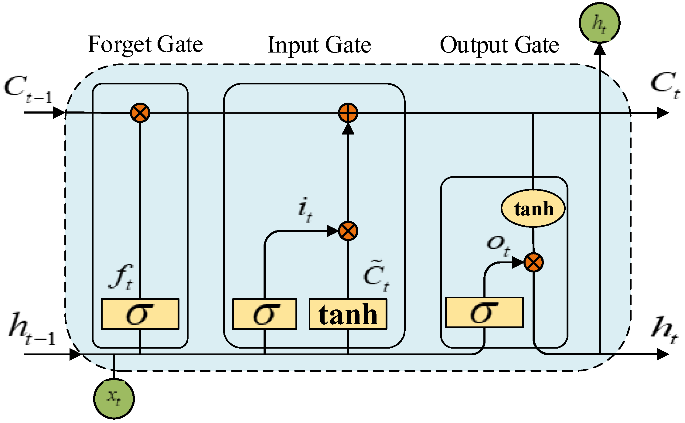
In order to overcome the defect that RNN cannot learn the remote dependence of long time series due to the disappearance of gradient, LSTM improves the model’s ability to capture long time series sample information by adding three control units on the basis of RNN [28]: the forgetting gate , the input gate , and the output gate . The basic structure of LSTM is shown in Figure 1.

Figure 1.
The basic architecture of LSTM.
The three control units of LSTM have different functions: the input gate determines how much information is retained in the memory unit, the output gate controls the output information of the current unit, and the forgetting gate determines the degree of forgetting of the information at the previous time point (memory degree). The three control unit vector calculation formulas are shown in (8):
In the formula, is the sigmoid function, and the value generated determines whether the information at the previous moment is retained or partially retained; , , and are the weight matrix of forgetting gate, input gate, and output gate; , , and are the bias terms of the three.
, , and are the memory state, input state and output state after updating at time t, respectively. The calculation formula is shown in (9):
In the formula, is the input at time t: tanh is a hyperbolic tangent activation function, which can scale the output state to (−1, 1).
The number of hidden layer neurons, learning rate, regularization coefficient, and training epochs are key parameters that define an LSTM model and directly affect its predictive performance. Therefore, optimizing these parameters should be the primary goal.
3. Prediction Model under the Condition of Missing Data
In order to solve the problem that the random missing values of the wind turbine bearing vibration signal affect the accuracy of RUL prediction, a new strategy is proposed: AS-GAIN-LSTM. Firstly, the missing values in are accurately interpolated, and then the optimized LSTM is used for RUL prediction. The overall flow chart is shown in Figure 2.
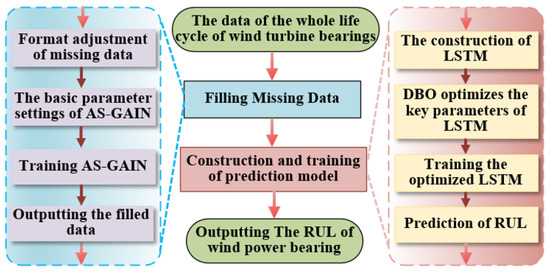
Figure 2.
Flowchart for AS-GAIN-LSTM.
The AS-GAIN architecture is shown in Figure 3, and the DBO-LSTM optimization process is shown in Figure 4.
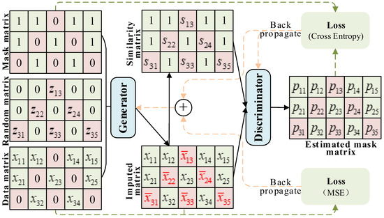
Figure 3.
Architecture diagram of AS-GAIN.
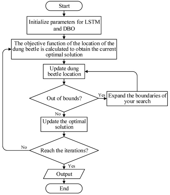
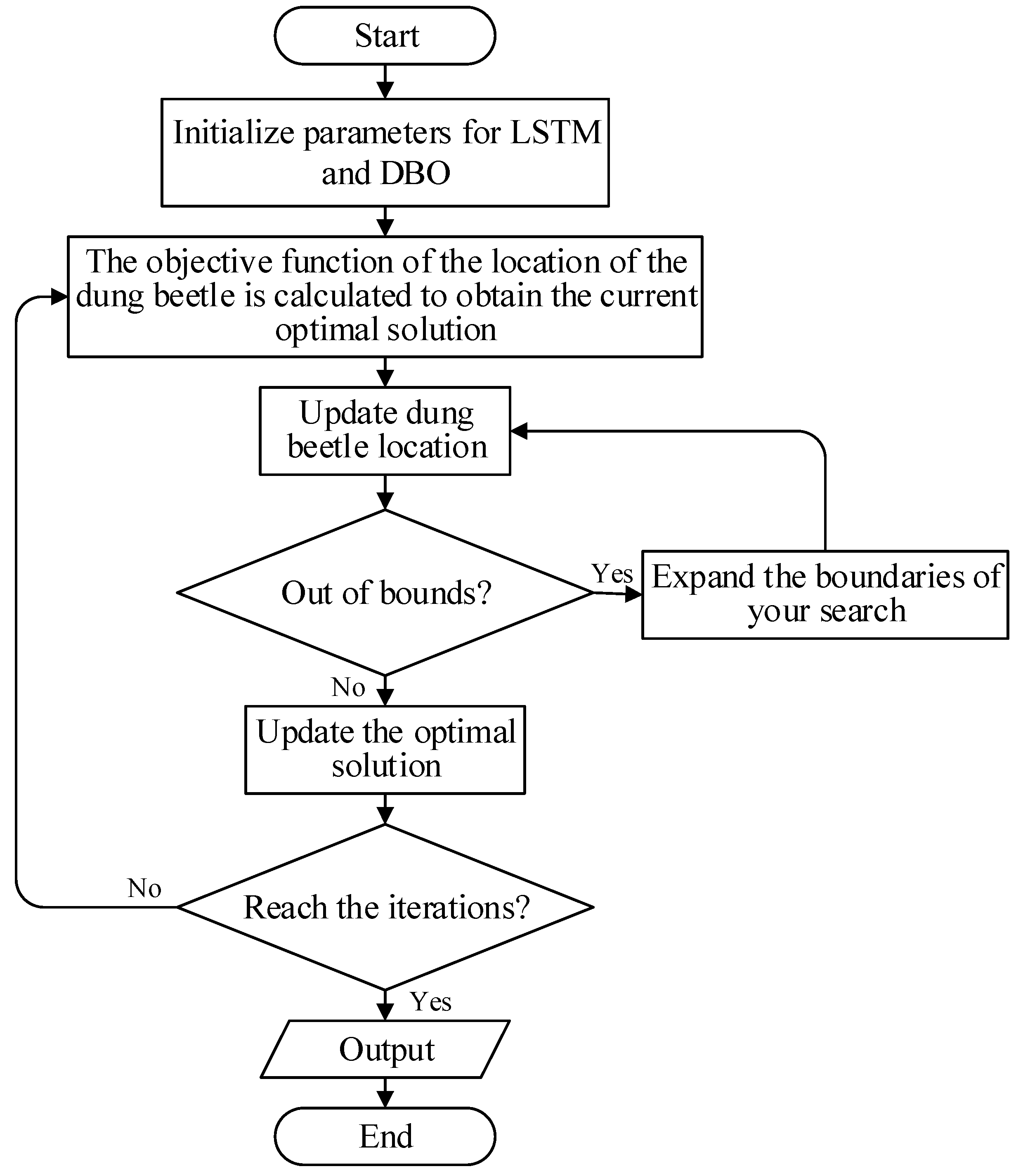
Figure 4.
Flowchart for optimizing LSTM with DBO.
3.1. AS-GAIN
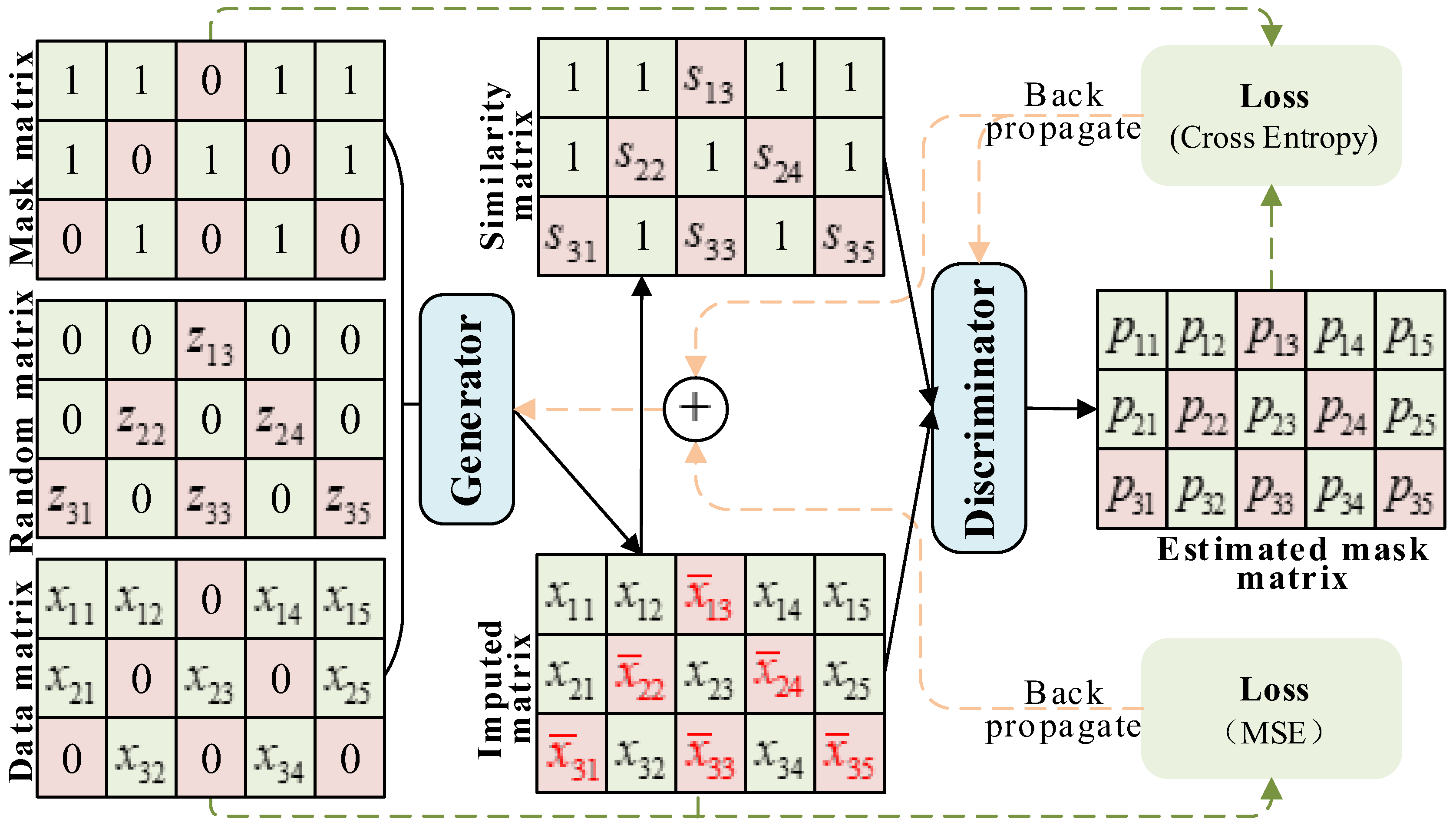
In GAIN, the hint vector H enhances the adversarial process between the generator G and the discriminator D. However, it is limited by its definition, providing D with only a limited amount of information. Moreover, the elements of H require manual setting, which increases uncertainty in model performance. To address these issues, this paper introduces average similarity as an augmentation to GAIN’s adversarial process, known as AS-GAIN. In the process of model training, the average similarity matrix (AS) between the filling value in the filling matrix and its grouping elements is constructed, and the average similarity matrix S and the filling matrix are used as the two inputs of the discriminator. The discriminator outputs a probability matrix about the filling matrix, and its elements describe the probability that the value of the corresponding filling matrix is the actual value. The refers to the complete data vector after filling, which observes the local information of , and then replaces the position of the corresponding value 0 in with the filling value in . The definition of is shown in Formula (10):
The introduction of mean similarity in the discriminator aims to primarily enhance its ability to capture information regarding the filled-in values, thereby overcoming the uncertainty of H and enabling the generator G to obtain more precise results during adversarial training. Average similarity describes the similarity between the imputed values and the actual values in each feature dimension, which indirectly reflects the reliability of the imputed values in an adversarial process. Upon receiving this information, the discriminator immediately provides feedback to the generator, allowing G to generate more realistic values for missing data in different locations. The discriminator function is redefined as: , S is the average similarity matrix with the same dimension as . The definition of S is shown in Formula (11):
In the formula, n is the number of groups of , m is the number of elements contained in each group of data, is the label matrix of , and the max is the maximum Euclidean distance related to the filling value ().
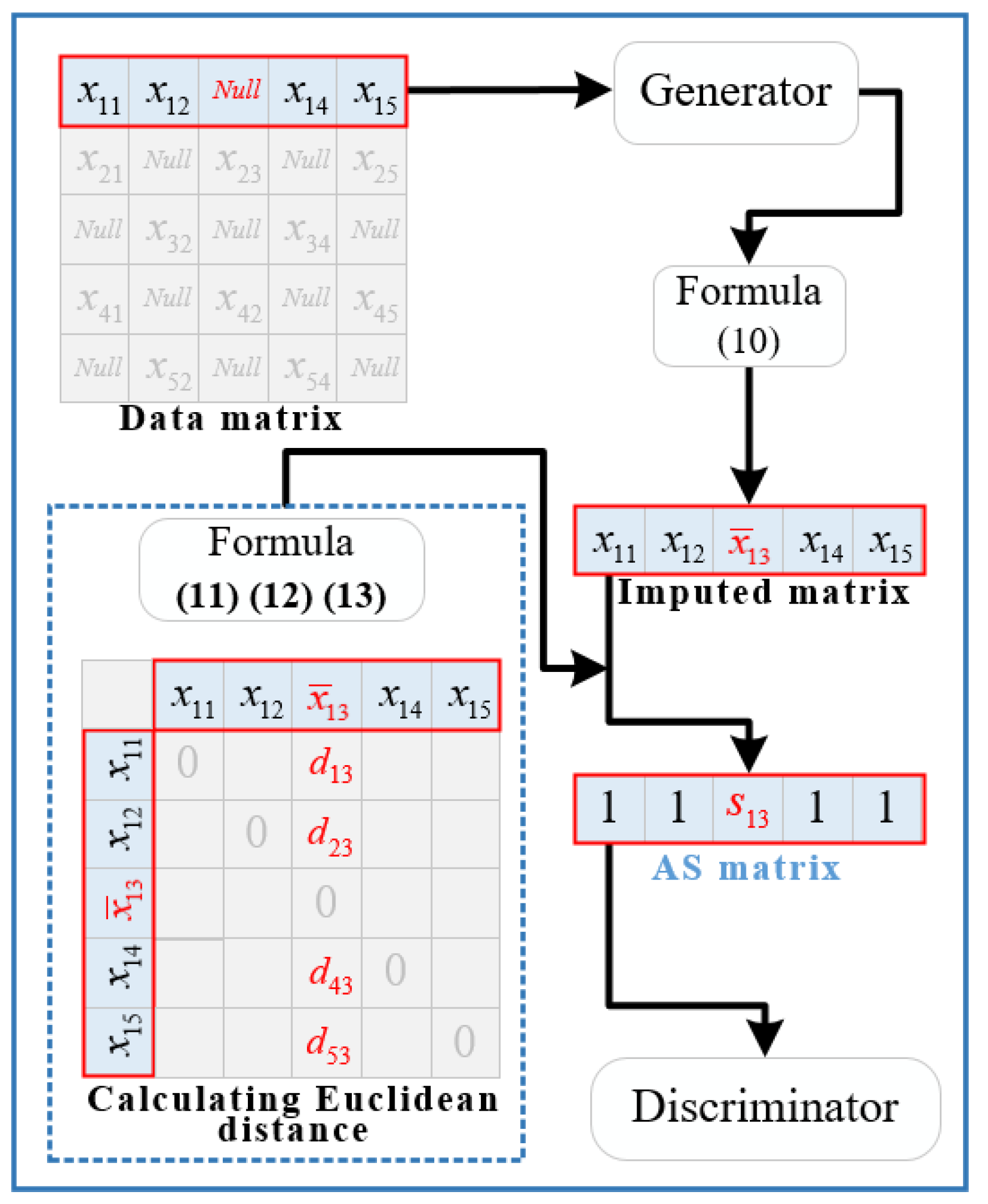
Assuming the minimum batch size for input of AS-Gain is 1 × 5, with a single missing value, we can generate a matrix of size 1 × 5 through generator D. This matrix can be transformed (using Formula (10)) to obtain a filled matrix of size 1 × 5. The similarity matrix S can then be computed using Formulas (11)–(13), as depicted in Figure 5.
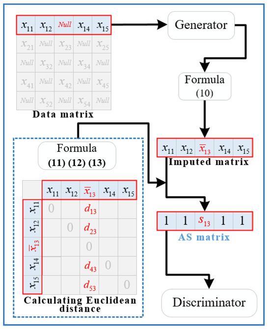
Figure 5.
The calculation process diagram of S.
In Figure 5, d represents the Euclidean distance between two elements. AS-GAIN provides an average similarity based on the minimum batch size for each missing value, which reveals the implicit association between the values generated by G in one training round and the ground truth. This association is then fused into D, thereby enhancing its discrimination capabilities. It should be noted that the minimum batch size may vary depending on the type of data and different features within the same type. Suppose the minimum batch size is excessively large. In that case, it can weaken the connection between the imputed value and the actual value, thereby affecting the generation and discrimination capabilities of G and D. Conversely, if the minimum batch size is too small, it can incorrectly describe the relationship between the imputed value and the actual value, thus degrading the performance of G and D. During testing, we found that the smallest batch size that best suits the characteristics of the experimental data employed in Section 5.1 is between 13 and 18.
By improving the discriminator D, AS-GAIN is obtained on the basis of GAIN, and its architecture is shown in Figure 3.
3.2. LSTM Is Optimized by DBO
The LSTM model consists of multiple neurons, connections, and memory units, each incorporating multiple gate mechanisms. Additionally, the model’s parameter space is typically vast, encompassing numerous weights and biases. These factors directly impact the model’s feature extraction performance, prediction accuracy, and memory overhead. Manual tuning of model parameters requires multiple trials and adjustments, resulting in lower efficiency and unsatisfactory outcomes. To address this issue, a proposal was made to optimize LSTM’s key parameters using the Ant Colony Optimization algorithm. The Dung Beetle Optimizer (DBO), operating within the parameter space, can search for the optimal parameter combination that minimizes the loss function or maximizes model performance metrics. Based on this, the design of the LSTM model presented in this paper is shown in Table 1.

Table 1.
The setting of parameters for LSTM.
The last four primary parameters in Table 1 were optimized through DBO.DBO is a new optimization algorithm [29], inspired by the foraging behavior of the Dung Beetle. It combines the strategies of global search and local development to achieve fast convergence and high accuracy optimization. The population of the dung beetle optimization algorithm is composed of four representative individuals: the ball-rolling dung beetle, the hatching dung beetle, the small dung beetle, and the thief dung beetle. Each individual represents a potential solution. They interact and collaborate to obtain the optimal solution by simulating the behavior and information exchange of dung beetles. The detailed process is showcased in Section 5.3 of this article.
In order to simulate the process of dung beetles pushing the dung ball and using the antenna to identify the direction of the straight line, the target point is allowed to move in the search space in accordance with the specified direction. Considering the sensitivity of dung beetles to light, the position change of dung beetles during the forward process is shown in Formula (14):
In the formula, t represents the current number of iterations; describes the position of the t-th iteration of the i-th dung beetle; k is the perturbation factor, and the value range is (0, 0.2); and are fixed value parameters: describes the intensity of light, and the calculation formula is shown in Formula (15): is the worst local position of the dung beetle.
When the dung beetle encounters obstacles in the process of advancement, it is necessary to re-formulate the route and update the position calculation formula of the dung beetle, as shown in Formula (16):
In the formula, is the size of the perturbation, and the value range is .
Reproduction is an important behavior in the dung beetle population. The spawning area of female dung beetles should be set within a safe range. The boundary definition is shown in Formula (17):
In the formula, and are the lower and upper bounds of the safe spawning area; and are the lower and upper bounds of the optimization problem; is the local optimal position of the dung beetle: is the boundary dynamic adjustment range, and the calculation process is as follows (18): is the maximum number of iterations.
After determining the spawning area of the female dung beetle, the position of the egg ball will change. The formula for calculating the position of the egg ball is updated as shown in Formula (19):
In the formula, describes the position of the t-th iteration of the i-th egg ball; and are two independent vectors of , N is the dimension of the optimization problem.
In order to simulate the foraging behavior of small dung beetles in the population, the foraging area is first defined as shown in Formula (20):
In the formula, and are the lower and upper bounds of the optimal foraging region, is the global optimal position of the dung beetle.
Secondly, the position of the small dung beetle foraging is updated, and the calculation formula is shown in Formula (21):
In the formula, describes the position of the t-th iteration of the i-th dung beetle, is a random number that obeys the normal distribution, and is a random number in (0, 1).
There are food contenders in the dung beetle population. Assuming that the optimal competition location is, the position update of the i-th thief at the t-th iteration is shown in Formula (22):
In the formula, is a random vector that obeys normal distribution and has a size of , and is a fixed constant.
The dung beetle algorithm optimization LSTM flow chart is shown in Figure 4.
3.3. Model-Evaluation Index
The AS-GAIN evaluation index uses root mean square error (RMSE) and mean absolute error (MAE). The DBO-LSTM evaluation index uses RMSE, MAE, and mean absolute percentage error (MAPE). The calculation methods are shown in Formula (23) [30]:
In the formula, n is the number of samples; is the actual value; is the predicted value (filled value by AS-GAIN).
4. Experiment Setting
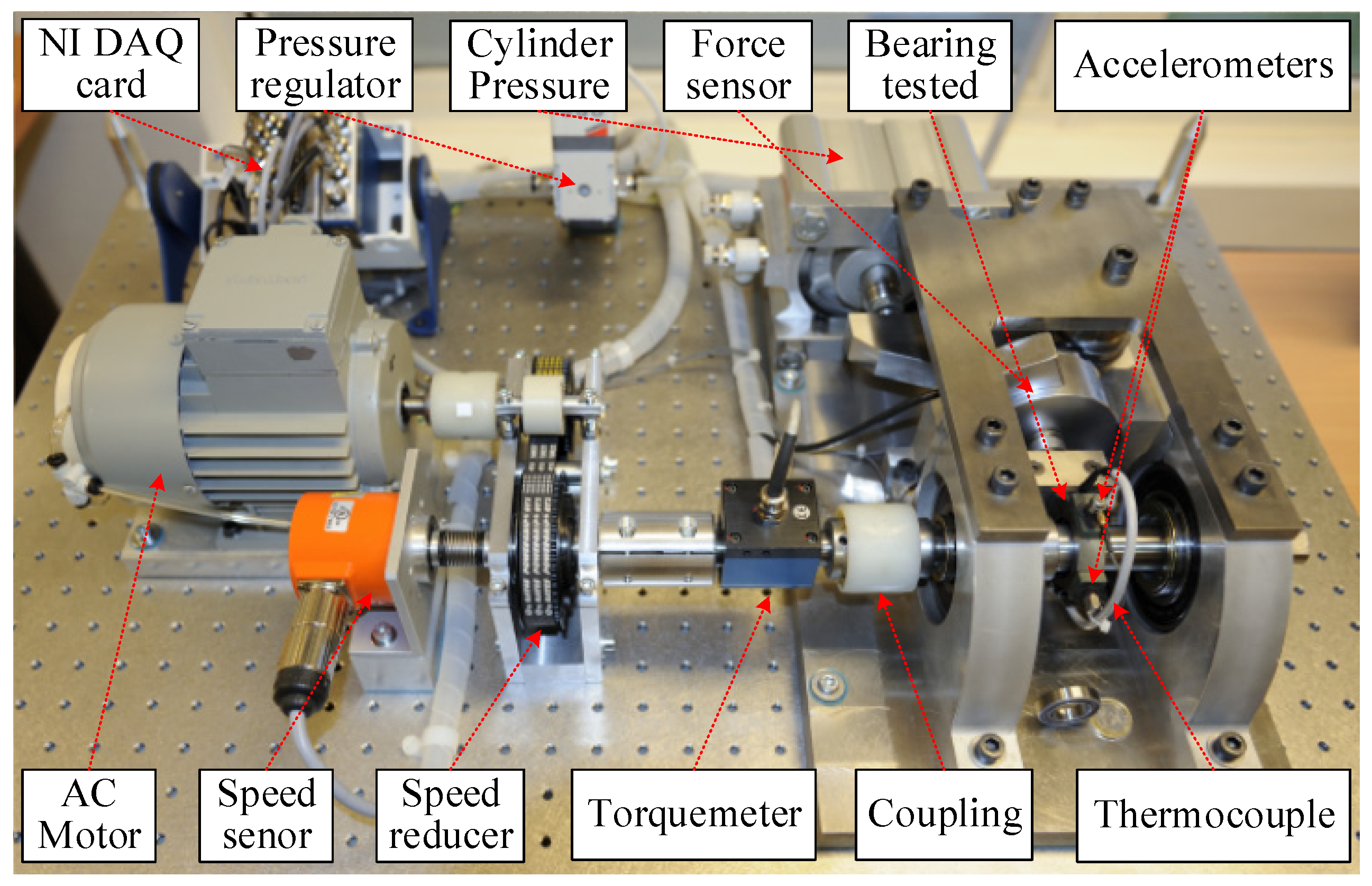
The bearing life data set provided by the PHM2012 data challenge [31] is used to verify the effectiveness of the proposed method. The vibration data includes the axial and radial signals collected by two vibration sensors. The stop threshold of signal acquisition is 20 g, the sampling frequency is 25.6 kHz, and the sampling time is 0.1 s. The data acquisition device is shown in Figure 6, and the working condition is divided in Table 2.
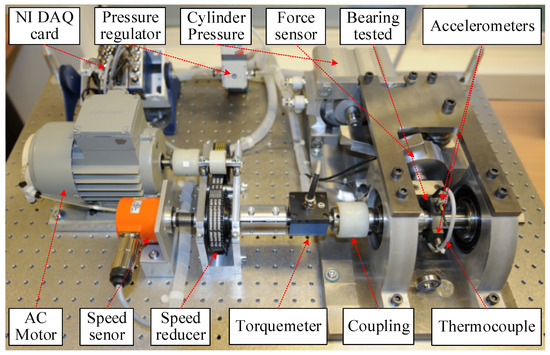
Figure 6.
The device for collecting experimental data.
Table 2.
Operating condition of the datasets.
In this study, the ball bearings being investigated share a similar construction principle as those found in other sizeable rotating machinery components. Additionally, monitoring data for wind turbine equipment parts as they approach failure is currently scarce or nonexistent [32]. This accurately predicts the lifespan of wind turbine bearings using publicly available datasets covering the entire life cycle of the bearings. Bearing 1_3 under condition 1 exhibits an evident degradation trend that aligns with the degradation trajectory of wind turbine bearings. Therefore, it serves as experimental data for validating DBO-LSTM and AS-GAIN-LSTM. Due to the significant differences in data volume and features between bearing 1_3 and bearing 2_3, the latter is used as an experimental subject for validating AS-GAIN. Firstly, bearing 1–3 and bearing 2–3 data are used to simulate the working conditions with missing data to verify the AS-GAIN filling performance. Secondly, the prediction performance of DBO-LSTM is verified by bearing 1–3 degradation stage data. Finally, the degradation stage data after bearing 1–3 filling is used to verify the comprehensive performance of AS-GAIN-LSTM under the condition of missing data.
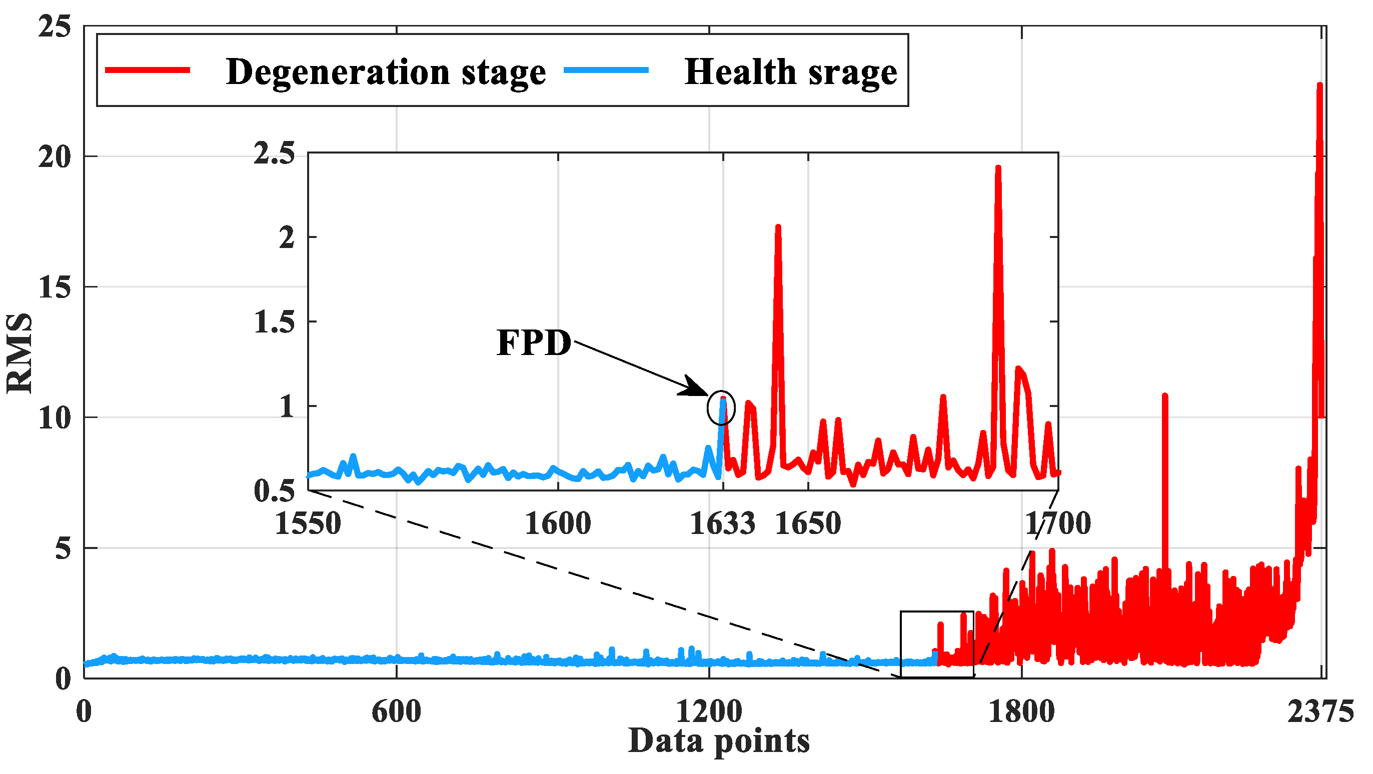
The life cycle of rolling bearings can be divided into two stages: the health stage and the degradation stage. Due to the large proportion of the healthy stage and the relatively stable signal, selecting this stage to train the model and perform life prediction has a great influence on the prediction accuracy of the model. Therefore, selecting the first point of degradation (FPD) and determining the degradation stage is particularly important. WANG et al. [5] assumed that the degradation amount of the healthy stage obeys the 3ס rule proposed by the normal distribution. According to this criterion, the degradation interval of the whole life cycle of the rolling bearing is determined, and the RUL prediction experiment is carried out.
The root mean square (RMS) can be employed to gauge the degradation of bearings [33], thus treating the RMS of vibration signals as experimental objects (with every 2560 original data points constituting a sample point), with a training set-to-test set ratio of 7:3. To validate the performance of DBO-LSTM and AS-GAIN-LSTM, five experimental schemes were designed, as shown in Table 3. The parameters of some parts in GAIN and AS-GAIN are set as shown in Table 4.
Table 3.
Design of the experimental plans.
Table 4.
Set of parameters for GAIN and AS-GAIN.
5. Experimental Analysis
5.1. Performance Verification of AS-GAIN
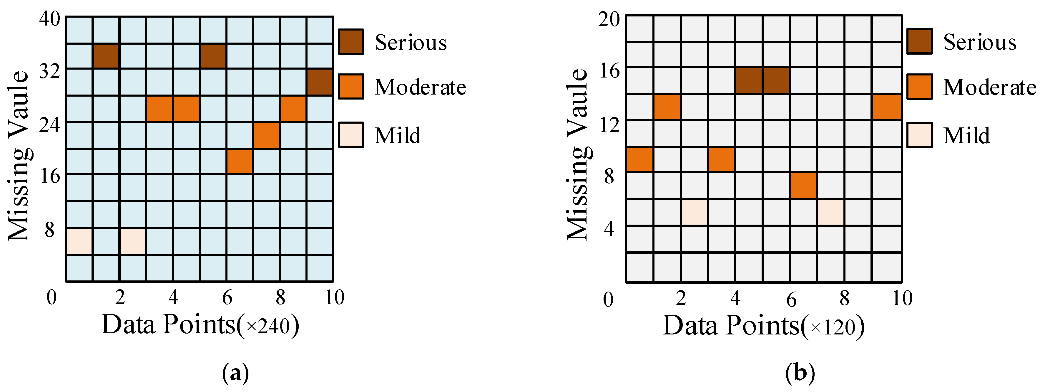
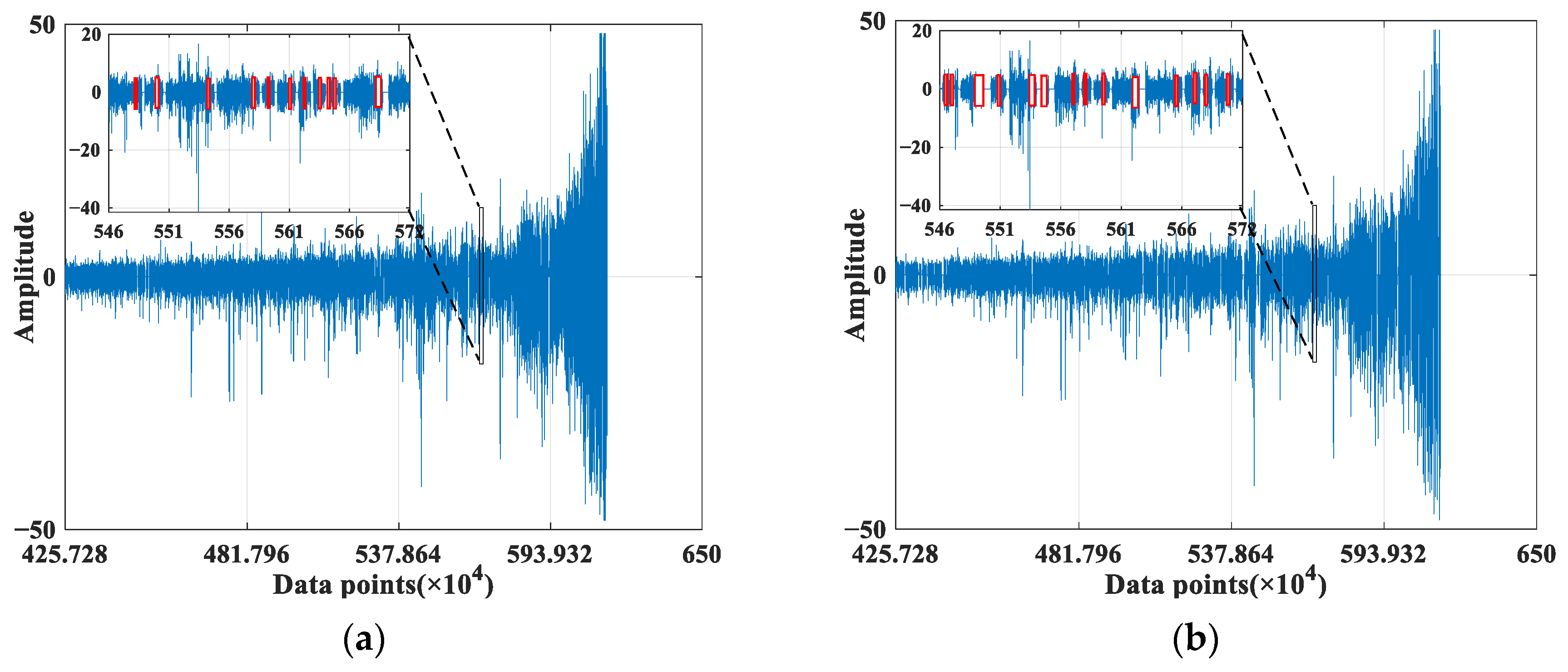
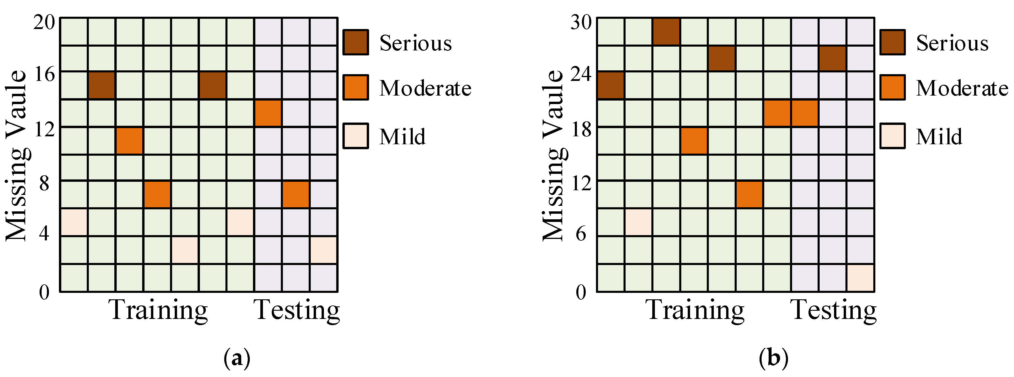
To validate the performance of AS-GAIN in filling in missing data, experiments employed the full-life cycle data of bearing 1_3 and bearing 2_3. Figure 7a,b separately simulate the original signal diagrams for bearing 1_3 and bearing 2_3 under missing completely at random (MCAR) with a missing rate of 10%. It should be noted that in the absence of MAR or MNAR patterns, the probability of missing values may be related to the characteristics of other observed values or the nature of the missing value itself. In such cases, the occurrence of missing data can introduce bias into the dataset, which would weaken the influence of the average similarity matrix S in AS-GAIN. How AS-GAIN can adapt to these two missing pattern scenarios remains an open question. Figure 8 depicts the missing value distribution pattern based on the original signal in Figure 7, with each missing value position corresponding to the RMS of bearing 1_3 and bearing 2_3 (bearing 1_3 and bearing 2_3 refer to the RMS of bearing 1_3 and the RMS of Bearing 2_3, respectively). As depicted in Figure 8, under this MCAR missing pattern, all intervals essentially contain the missing parts; however, there exist some differences in the distribution of missing values for bearing 1_3 and bearing 2_3: severe missing in bearing 1_3 is evenly distributed throughout the entire interval, whereas in bearing 2_3, it mainly occurs between data points 480 and 720. Suppose there is a disproportionate concentration of missing values in a particular region. In that case, the accuracy of the relationship captured by matrix S may be compromised when using AS-GAIN to fill in these values. This could result in suboptimal outcomes not only for AS-GAIN but also for other filling algorithms. In addition, when the missing rate is 10%, the number of missing values for bearing 2_3 is significantly lower than that for bearing 1_3. This is due to the inherent differences in magnitude between the two sets of original data. Each data point carries with it distinct characteristics of its original data, resulting in entirely different traits exhibited by the two sets. This will serve as a test for the stability and reliability of the model.
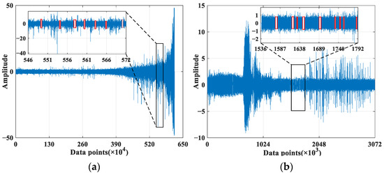
Figure 7.
The distribution of missing data in the original signal. (a) The original signal for bearing 1_3. (b) The original signal for bearing 2_3. (The red flag indicates the missing value).

Figure 8.
Distribution of different bearings with 10% missing values. (a) Bearing 1_3 with 10% missing values. (b) Bearing 2_3 with 10% missing values.
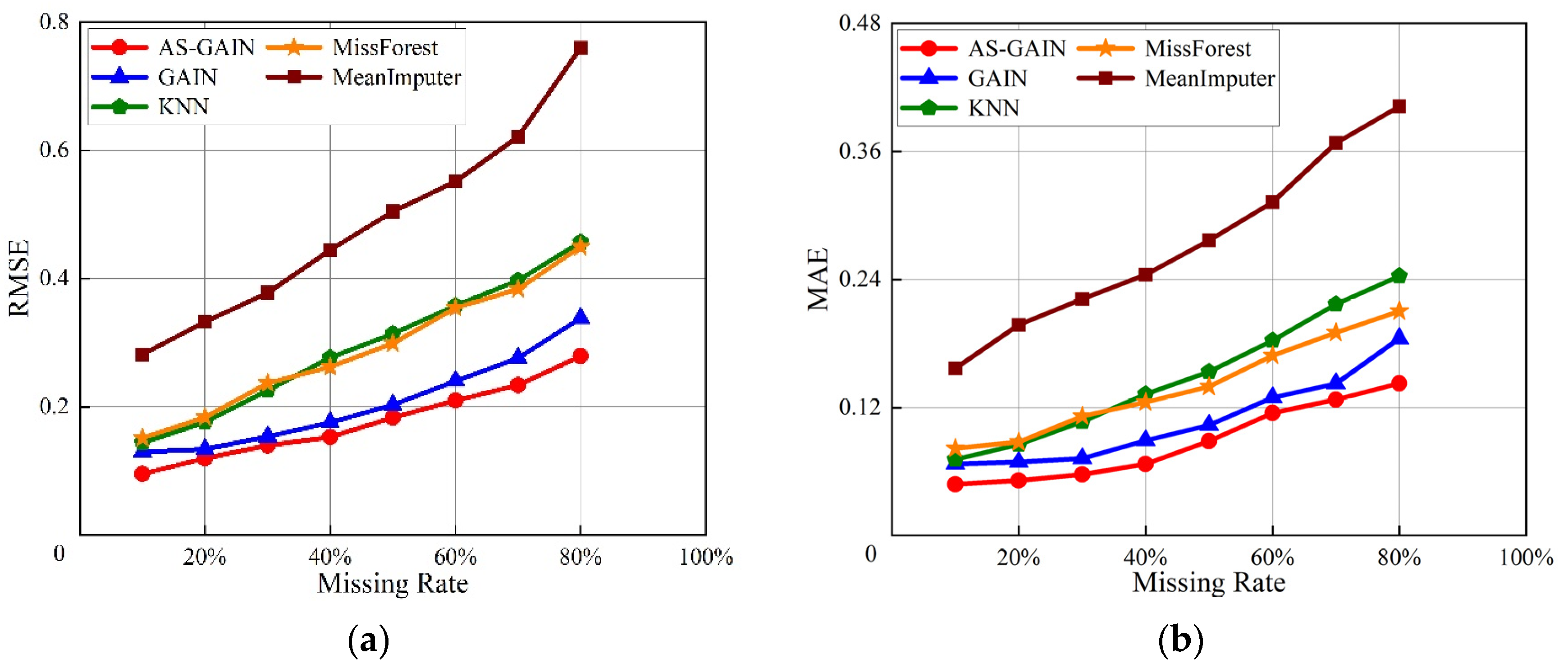
For bearing 1_3, Figure 9a,b show the RMSE and MAE of different filling models under different missing rates and evaluate the filling performance of different models through these two indicators. From Figure 7a,b, it can be seen that with the increase in bearing 1_3 missing rate, the performance of each filling model gradually decreases. However, compared with other models, the performance of AS-GAIN is still the best under the same missing rate. Moreover, with the increase in the missing rate, the growth rate of the RMSE and MAE of AS-GAIN is also the lowest, which indicates that AS-GAIN has better stability. Especially in scenarios with a high missing rate (>80%), AS-GAIN has obvious advantages. When the missing rate is 80%, the RMSE of AS-GAIN is 15%, 35%, 40%, and 60% lower than that of GAIN, KNN, MissForest, and MeanImputer, respectively. Compared with GAIN, KNN, MissForest, and MeanImputer, MAE decreased by more than 20%, 40%, 30%, and 60%, respectively.

Figure 9.
Different evaluation metrics for bearing 1_3 at different missing rates. (a) RMSE of bearing1_3 at different missing rates. (b) MAE of bearing 1_3 at different missing rates.
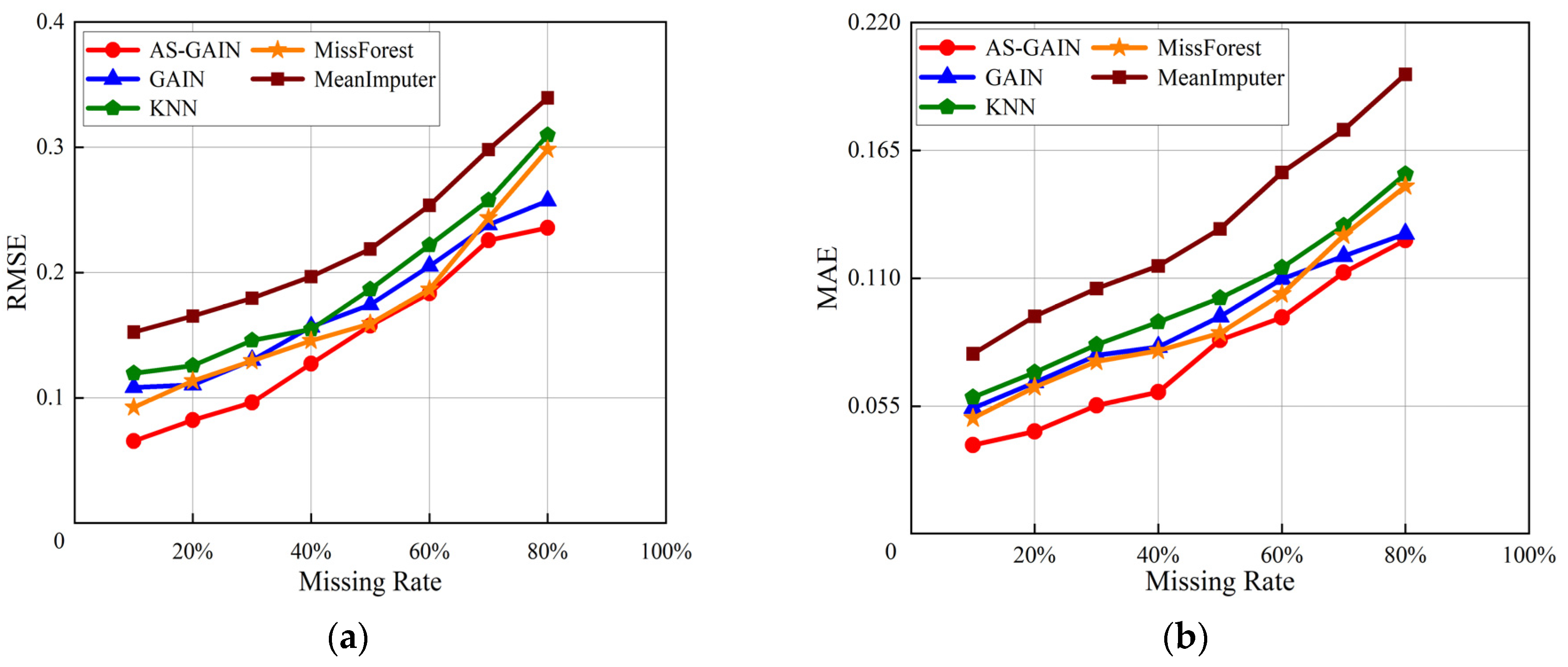
For bearing 2_3, Figure 10a,b show the RMSE and MAE of different imputation models under different missing rates. Compared with Figure 9a,b, the differences of each model under different missing rates are smaller, and the values of RMSE and MAE are also smaller. This is because the sample size of bearing 2_3 is smaller and the data itself has a higher similarity. Among the five filling models, the comprehensive index performance of AS-GAIN is still optimal. Especially when the missing rate is 80%, the RMSE of AS-GAIN is better than that of GAIN, KNN, MissForest, and MeanImputer by 8%, 20%, 25%, and 30%, respectively. Compared with GAIN, KNN, MissForest, and MeanImputer, MAE decreased by more than 2%, 15%, 15%, and 35%, respectively. This verifies that AS-GAIN has a good filling effect when dealing with different missing rates and different missing data.
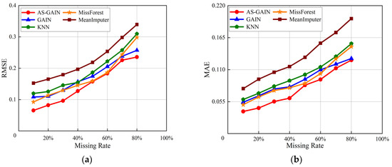
Figure 10.
Different evaluation metrics of bearing 2_3 at different missing rates. (a) RMSE of bearing 2_3 at different missing rates. (b) MAE of bearing 2_3 at different missing rates.
As shown in Figure 9 and Figure 10, as the missing rate gradually increases, imputation errors also increase for different models. This is due to the fact that missing values contain information about the original data’s characteristics, which, when lost, can cause a decrease in the accuracy of prediction models. As the number of missing values increases, the loss of reliable information becomes more significant, resulting in a decline in model prediction accuracy. Based on the trend of the evaluation indicators, it can be observed that the performance decline of AS-GAIN is the most gradual.
5.2. Performance Verification of DBO-LSTM
In order to verify the prediction performance of DBO-LSTM, experiments were carried out using Plans A, B, C, and D. According to the 3ס rule, the FPD was determined to be the 1633th data point position, and the degradation interval was [1633, 2375]. Figure 11 describes the health stage and degradation stage of the full-life cycle of bearing 1_3.

Figure 11.
The FPD of bearing 1_3 under the 3ס criterion.
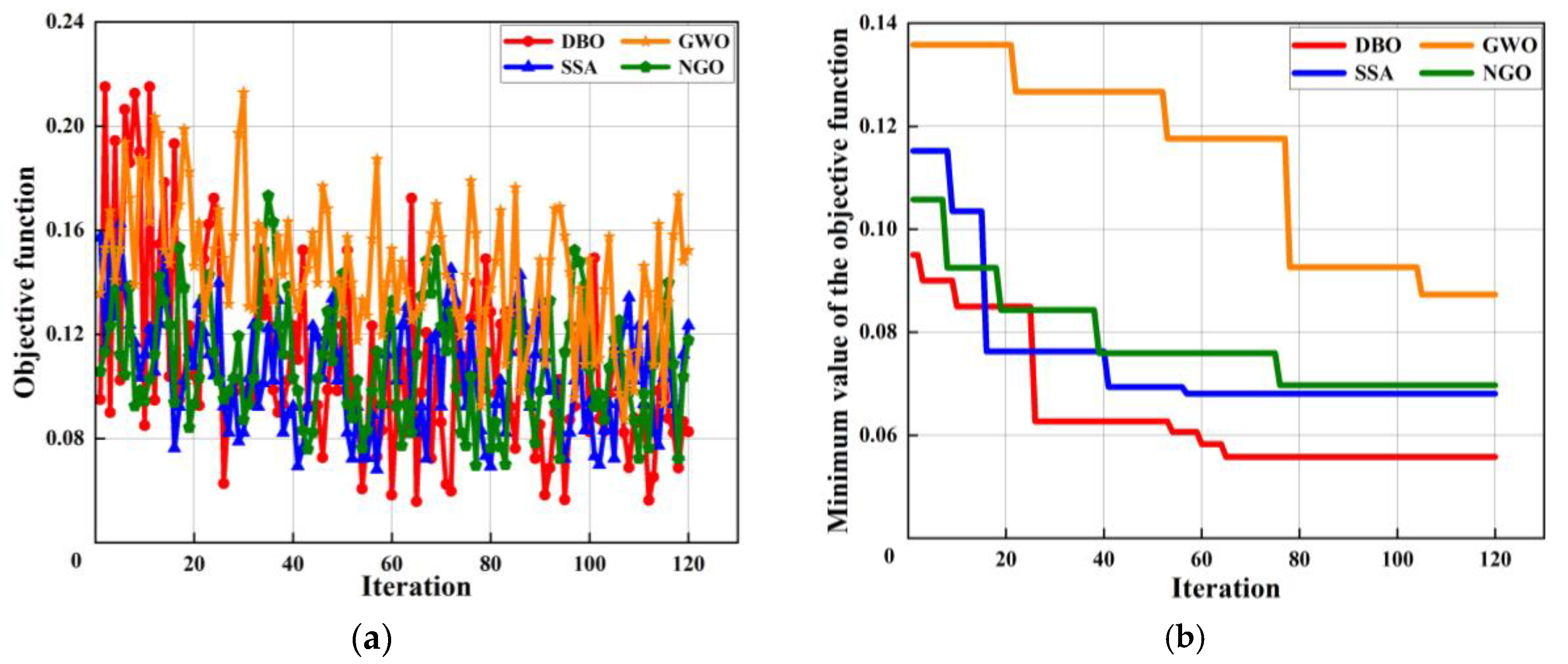
In order to improve the generalization ability of the model, MAPE is used as the objective function, Adam0 is used as the optimizer, and the critical parameters of LSTM are optimized based on DBO. In order to give full play to the ability of DBO optimization, the parameters of LSTM are searched 120 times, and the search range of the number of hidden layer neurons is set to 50~150 according to the size of the training set. In order to improve the convergence speed of the prediction model, the initial learning rate search range is set to 0.001~0.01. In order to prevent over-fitting of the prediction model, the training times and regularization coefficients are set to 25~100 and 1 × 10⁻¹⁰~1 × 10⁻³, respectively. The DBO optimization process is shown in Figure 12. It can be seen from Figure 12a that the objective function value tends to be stable and reaches the minimum value after the number of iterations reaches 66. It can be seen from Figure 12b that the minimum value of the objective function is reduced from 0.09503 to 0.0558 in the optimization process. In comparison to other optimization algorithms, it is evident that for the data utilized in this paper, DBO demonstrates a swifter convergence rate and also identifies the optimal solution prior to the cessation of iterations.

Figure 12.
Optimization process of different algorithms for LSTM. (a) Objective function and iteration. (b) The minimum value and iteration.
The parameter combination corresponding to the minimum value of the optimized objective function is the optimal parameter combination. The DBO optimization results are shown in Table 5. According to Table 5, the optimization parameters of the number of hidden layer neurons, the initial learning rate, the number of training times, and the regularization coefficient are 118, 0.006623, 93, and 1 × 10⁻¹⁰, respectively. This set of optimization parameters will be used to construct the LSTM model.
Table 5.
The parameters of LSTM optimized by DBO.
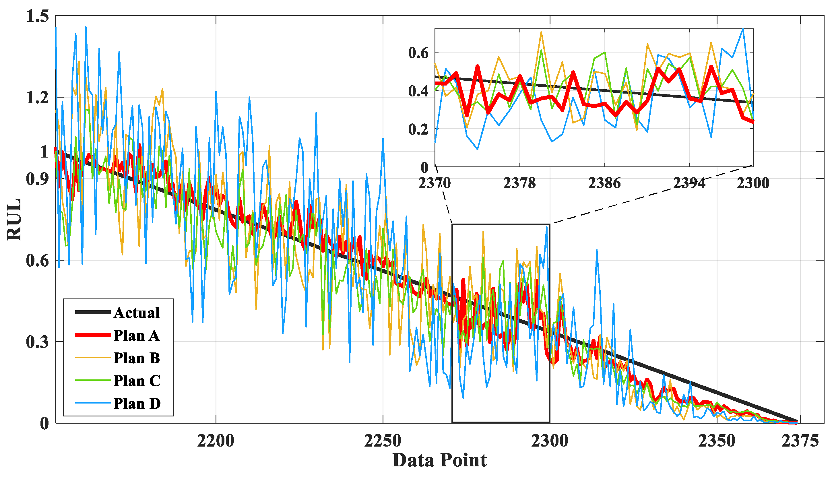
Figure 13 is the comparison chart between the predicted results and the actual values of Plans A, B, C, and D. As shown in Figure 13, it is evident that Plan D exhibits the most significant deviation from the actual values in terms of prediction results. This indicates that, among the various prediction models, LSTM demonstrates superior predictive ability. Furthermore, the prediction outcomes of Plan A surpass those of Plan B and C, suggesting that employing DBO to optimize LSTM is a feasible approach for enhancing its predictive performance.
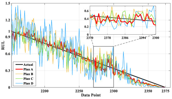
Figure 13.
Comparison of the predictions of different plans of bearing 1_3.
Table 6 shows the prediction errors of A, B, and C Plans. It can be seen from Table 5 that the MAE, RMSE, and MAPE of Plan A are 5.78%, 21.06%, and 18.06% lower than those of Plan C, respectively. The MAE, RMSE, and MAPE of Plan A were 44.17%, 40.40%, and 53.85% lower than those of Plan B, respectively. The MAE, RMSE, and MAPE of Plan A were 67.45%, 59.30%, and 71.86% lower than those of Plan D, respectively. When comparing Model B and Model D individually, Model B shows a reduction in the MAE, RMSE, and MAPE of Model D by 41.70%, 31.72%, and 39.03%, respectively. These results sufficiently demonstrate that DBO-LSTM can more accurately describe the degradation trajectory of rolling bearings compared to LSTM and SSA-LSTM. Additionally, LSTM shows better predictive performance compared to RNN.
Table 6.
Different plans were used to evaluate the prediction of bearing 1_3.
In order to better emphasize the predictive capability of LSTM, Table 7 presents the runtime of various models under identical conditions (CPU: i5-1240P, RAM: 32 GB, Operating System: Windows 11) and the same experimental data (Data Size: 2375 × 1). As evidenced by the table, LSTM has the shortest runtime, as it does not factor in the optimization algorithm’s runtime. In comparison to the RNN model, LSTM also possesses the ability to complete prediction tasks more quickly. When these models are executed with superior devices or alternative data, shorter runtimes may be attained.
Table 7.
Running time of different models.
5.3. Performance Verification of AS-GAIN-LSTM
To validate the efficacy of the AS-GAIN-LSTM approach, experiments were carried out with Plans A, E, and F. Initially, bearing 1_3’s missing rates in the degradation interval (data after FPD in Figure 11) were set at 10% and 20% under the MCAR condition. The missing data simulated from the original signal are illustrated in Figure 14a,b. The corresponding RMS missing distribution of bearing 1_3 is depicted in Figure 15a,b.
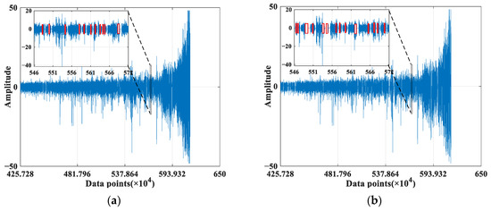
Figure 14.
Distribution of different numbers of missing values under bearing 1_3. (a) The missing rate is 10%. (b) The missing rate is 20%. (The red flag indicates the missing value).

Figure 15.
Distribution of bearing 1_3 with different missing rates. (a) The missing rate is 10%. (b) The missing rate is 20%.
When comparing two different scenarios of random missing data, with missing rates of 10% and 20%, the missing values are distributed evenly in both the training and testing sets. The amount of missing data can potentially impact the performance of AS-GAIN-LSTM, and the subsequent sections will provide a more detailed explanation of the results.
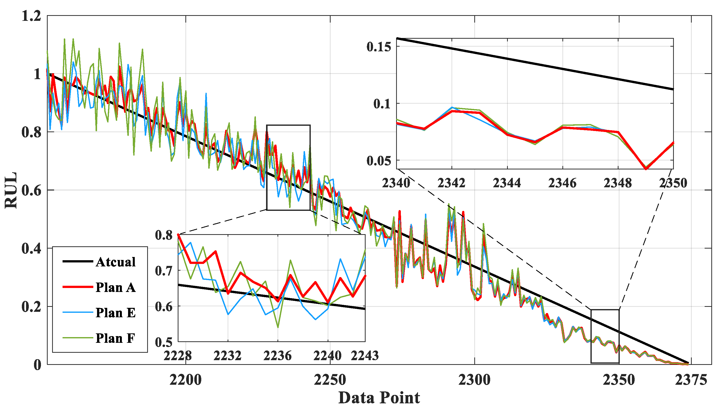
Figure 16 is a comparison chart of the actual results of RUL prediction after the proposed prediction model is used to fill the degradation interval data with missing ratios of 0%, 10% and 20%, respectively. The missing value filling method adopts AS-GAIN. The corresponding missing ratios of Plan A, E, and F were 0%, 10%, and 20%, respectively. Based on the depicted graph, it seems that the prediction from Plan A provides the most accurate approximation to the actual value. Initially, both Plan E and Plan F demonstrated more significant discrepancies with the actual values in comparison to later forecasts. This could potentially be attributed to some shared missing values in Figure 15a,b.
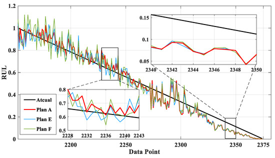
Figure 16.
Comparison of the predictions of different plans of bearing 1_3 with missing data conditions.
After AS-GAIN fills the data with three missing ratios (0%, 10%, and 20%), DBO-LSTM is used to predict the RUL of the filled-in complete data. The prediction error is shown in Table 8. It can be seen from the Table that when there are 10% missing values in the data, the MAE, RMSE, and MAPE of using AS-GAIN for data filling and DBO-LSTM for RUL prediction are only 1.75%, 1.89%, and 8.31% higher than those of using DBO-LSTM for life prediction of the original complete data. When there are 20% missing values in the data, the MAE, RMSE, and MAPE of the AS-GAIN-filled and DBO-LSTM-based RUL predictions are only 3.28%, 3.30%, and 12.72% higher than those of the original complete data using DBO-LSTM for life prediction. It can be seen that when there are missing values in the rolling bearing data, it is feasible to use the AS-GAIN-LSTM strategy for the prediction of RUL.
Table 8.
Different plans were used to evaluate the prediction of bearing 1_3 with different missing conditions.
As shown in Figure 16 and Table 8, when inputting missing rate data with varying degrees of incompleteness into DBO-LSTM, the prediction errors corresponding to high-missing-rate data were slightly higher than those associated with low-missing-rate data. According to the principle outlined in Section 3.1, matrix S calculates the Euclidean distance between the filled values of G within the same minimum batch and their actual counterparts, including the Euclidean distance between the filled values of G themselves. However, the G imputation value itself carries an error when compared to the actual value. As more missing values exist in the data, it is inevitable that S will contain more errors, which would lower its discriminatory power for distinguishing D. This, in turn, reduces the reliability of the information contained within the generated data. During LSTM training, the model analyzes the depth features of the data. When the data itself contains errors, it is inevitable that these will negatively impact the model, thereby reducing its predictive capabilities.
6. Conclusions
- In the data preprocessing stage, aiming at the problem of random missing data in the process of signal acquisition of wind power bearings, AS-GAIN can be used to fill the missing values to obtain more accurate filling values because AS-GAIN can better describe the difference between the filling value and the actual value. In the process of confrontation between the generator and the discriminator, the information about the average similarity of the filled values is integrated into the discriminator, so that the generator pays more attention to the filling effect of the missing values. After many confrontation training sessions, a generator with excellent filling effects can be obtained. The experimental results show that the performance of AS-GAIN in processing the working condition data mentioned in this paper has obvious advantages compared with other models.
- In the RUL prediction stage, the number of hidden layer neurons, learning rate, regularization coefficient, and training times of LSTM are optimized by using the characteristics of fast convergence and strong optimization ability of the dung beetle algorithm, so that LSTM has better prediction performance in dealing with the prediction problem of long time series. The experimental results show that compared with LSTM and SSA-LSTM, the MAE of DBO-LSTM is reduced by 5.78% and 44.17%, respectively; RMSE is reduced by 21.06% and 40.40% respectively; and MAPE is reduced by 18.06% and 53.85%, respectively.
- AS-GAIN-LSTM is adopted to solve the problem that the wind power bearing data cannot be predicted by RUL that the accuracy of RUL prediction is low due to the presence of missing values. Firstly, AS-GAIN is used to accurately fill in the missing values, and then DBO-LSTM is used to predict RUL. The experimental results show that when there are missing values in the data, the prediction error using AS-GAIN-LSTM is only slightly improved compared with the prediction error using DBO-LSTM for complete data. AS-GAIN-LSTM gives full play to its filling ability and prediction ability, making it more excellent in dealing with such time series prediction problems with missing values.
Author Contributions
Conceptualization, X.L. (Xuejun Li); Methodology, L.J.; Validation, T.Y.; Writing—original draft, X.L. (Xu Lei); Supervision, Z.G. All authors have read and agreed to the published version of the manuscript.
Funding
We acknowledgment the support of Guangdong Provincial Basic and Applied Basic Research Fund (2023A1515240083), the Guangdong Provincial Key Construction Discipline Research Capability Improvement Project (2022ZDJS035), and the Guangdong Provincial University Innovation Team Project (2023KCXTD031). Our sincere gratitude goes to the reviewers for their insightful and constructive feedback, which has significantly enhanced the quality of this paper.
Data Availability Statement
The data presented in this study are available on request from the corresponding author.
Conflicts of Interest
The authors declare no conflict of interest.
References
- Stetco, A.; Dinmohammadi, F.; Zhao, X.; Robu, V.; Flynn, D.; Barnes, M.; Keane, J.; Nenadic, G. Machine learning methods for wind turbine condition monitoring. A review. Renew. Energy 2019, 133, 620–635. [Google Scholar] [CrossRef]
- Lei, Y.; Li, N.; Guo, L.; Li, N.; Yan, T.; Lin, J. Machinery health prognostics: A systematic review from data acquisition to RUL prediction. Mech. Syst. Signal Process. 2018, 104, 799–834. [Google Scholar] [CrossRef]
- Djeziri, M.; Benmoussa, S.; Sanchez, R. Hybrid method for remaining useful life prediction in wind turbine systems. Renew. Energy 2018, 116, 173–187. [Google Scholar] [CrossRef]
- Lei, Y.; Li, N.; Gontarz, S.; Lin, J.; Radkowski, S.; Dybala, J. A model-based method for remaining useful life prediction of machinery. IEEE Trans. Reliab. 2016, 65, 1314–1326. [Google Scholar] [CrossRef]
- Wang, Y.; Peng, Y.; Zi, Y.; Jin, X.; Tsui, K.-L. A two-stage data-driven-based prognostic Approach for bearing degradation problem. IEEE Trans. Ind. Inform. 2016, 12, 924–932. [Google Scholar] [CrossRef]
- Su, X.; Wang, S.; Pecht, M.; Zhao, L.; Ye, Z. Interacting multiple model particle filter for prognostics of lithium-ion batteries. Microelectron. Reliab. 2017, 70, 59–69. [Google Scholar] [CrossRef]
- Yang, T.; Li, G.; Li, K.; Li, X.; Han, Q. The LPST-Net: A new deep interval health monitoring and prediction framework for bearing-rotor systems under complex operating conditions. Adv. Eng. Inform. 2024, 62, 102558. [Google Scholar] [CrossRef]
- Yang, B.; Liu, R.; Zio, E. Remaining useful life prediction based on a double-convolutional neural network architecture. IEEE Trans. Ind. Electron. 2019, 66, 9521–9530. [Google Scholar] [CrossRef]
- Bai, R.; Noman, K.; Feng, K.; Peng, Z.; Li, Y. A two-phase-based deep neural network for simultaneous health monitoring and prediction of rolling bearings. Reliab. Eng. Syst. Saf. 2023, 238, 109428. [Google Scholar] [CrossRef]
- Singh, J.; Azamfar, M.; Li, F.; Lee, J. A Systematic Review of Machine Learning Algorithms for Prognostics and Health Management of Rolling Element Bearings: Fundamentals, Concepts and Applications. Meas. Sci. Technol. 2021, 32, 012001. [Google Scholar] [CrossRef]
- Mahmood, F.H.; Kadhim, H.T.; Resen, A.K.; Shaban, A.H. Bearing failure detection of micro wind turbine via power spectral density analysis for stator current signals spectrum. AIP Conf. Proc. 2018, 1968, 020018. [Google Scholar]
- Guo, L.; Li, N.; Jia, F.; Lei, Y.; Lin, J. A recurrent neural network based health indicator for remaining useful life prediction of bearings. Neurocomputing 2017, 240, 98–109. [Google Scholar] [CrossRef]
- Chen, Y.; Peng, G.; Zhu, Z.; Li, S. A novel deep learning method based on attention mechanism for bearing remaining useful life prediction. Appl. Soft Comput. 2020, 86, 105919. [Google Scholar] [CrossRef]
- Xiang, S.; Li, P.; Huang, Y.; Luo, J.; Qin, Y. Single gated RNN with differential weighted information storage mechanism and its application to machine RUL prediction. Reliab. Eng. Syst. Saf. 2023, 242, 109741. [Google Scholar] [CrossRef]
- Fu, C.; Gao, C.; Zhang, W. RUL Prediction for Piezoelectric Vibration Sensors Based on Digital-Twin and LSTM Network. Mathematics 2024, 12, 1229. [Google Scholar] [CrossRef]
- Li, Y.; Chen, Z.; Hu, C.; Zhao, X. Bearing remaining useful life prediction with an improved CNN-LSTM network using an artificial gorilla troop optimization algorithm. Proc. Inst. Mech. Eng. Part O J. Risk Reliab. 2024. [Google Scholar] [CrossRef]
- Liu, J.; Pan, C.; Lei, F.; Hu, D.; Zuo, H. Fault prediction of bearings based on LSTM and statistical process analysis. Reliab. Eng. Syst. Saf. 2021, 214, 107646. [Google Scholar] [CrossRef]
- Magadán, L.; Granda, J.C.; Suárez, F. Robust prediction of remaining useful lifetime of bearings using deep learning. Eng. Appl. Artif. Intell. 2024, 130, 107690. [Google Scholar] [CrossRef]
- Li, G.; Wang, Y.; Xu, C.; Wang, J.; Fang, X.; Xiong, C. BO-STA-LSTM: Building energy prediction based on a Bayesian Optimized Spatial-Temporal Attention enhanced LSTM method. Dev. Built Environ. 2024, 18, 100465. [Google Scholar] [CrossRef]
- Li, Z.; Du, J.; Zhu, W.; Wang, B.; Wang, Q.; Sun, B. Regression predictive modeling of high-speed motorized spindle using POA-LSTM. Case Stud. Therm. Eng. 2024, 54, 104053. [Google Scholar] [CrossRef]
- Jin, X.; Sun, Y.; Que, Z.; Wang, Y.; Chow, T.W. Anomaly Detection and Fault Prognosis for Bearings. IEEE Trans. Instrum. Meas. 2016, 65, 2046–2054. [Google Scholar] [CrossRef]
- Rădulescu, M.; Radulescu, C.Z. Mean-Variance Models with Missing Data. Stud. Inform. Control. 2013, 22, 299–306. [Google Scholar] [CrossRef]
- Yang, K.; Li, J.; Wang, C. Missing Values Estimation in Microarray Data with Partial Least Squares Regression; Springer: Berlin, Germany, 2006; pp. 662–669. [Google Scholar]
- Han, H.; Sun, M.; Wu, X.; Li, F. Double-cycle weighted imputation method for wastewater treatment process data with multiple missing patterns. Sci. China Technol. Sci. 2022, 65, 2967–2978. [Google Scholar] [CrossRef]
- Liu, W.; Ren, C.; Xu, Y. PV Generation Forecasting With Missing Input Data: A Super-Resolution Perception Approach. IEEE Trans. Sustain. Energy 2021, 12, 1493–1496. [Google Scholar] [CrossRef]
- Hart, E.; Turnbull, A.; Feuchtwang, J.; McMillan, D.; Golysheva, E.; Elliott, R. Wind turbine main-bearing loading and wind field characteristics. Wind. Energy 2019, 22, 1534–1547. [Google Scholar] [CrossRef]
- Yoon, J.; Jordon, J.; Schaar, M. GAIN: Missing Data Imputation using Generative Adversarial Nets. arXiv 2018, arXiv:1806.02920. [Google Scholar]
- Landi, F.; Baraldi, L.; Cornia, M.; Cucchiara, R. Working Memory Connections for LSTM. Neural Netw. 2021, 144, 334–341. [Google Scholar] [CrossRef]
- Xue, J.; Shen, B. Dung beetle optimizer: A new meta-heuristic algorithm for global optimization. J. Supercomput. 2023, 79, 7305–7336. [Google Scholar] [CrossRef]
- Li, X.; Zhang, W.; Ding, Q. Deep learning-based remaining useful life estimation of bearings using multi-scale feature extraction. Reliab. Eng. Syst. Saf. 2019, 182, 208–218. [Google Scholar] [CrossRef]
- Wang, B.; Lei, Y.; Li, N.; Li, N. A hybrid prognostics approach for estimating remaining useful life of rolling element bearings. IEEE Trans. Reliab. 2020, 69, 401–412. [Google Scholar] [CrossRef]
- Yang, N.; Stumberg, L.V.; Wang, R.; Cremers, D. D3VO: Deep Depth, Deep Pose and Deep Uncertainty for Monocular Visual Odometry. In Proceedings of the 2020 IEEE/CVF Conference on Computer Vision and Pattern Recognition (CVPR), Seattle, WA, USA, 13–19 June 2020; pp. 1278–1289. [Google Scholar]
- Camci, F.; Medjaher, K.; Zerhouni, N.; Nectoux, P. Feature evaluation for effective bearing prognostics. Qual. Reliab. Eng. Int. 2013, 29, 477–486. [Google Scholar] [CrossRef]


Disclaimer/Publisher’s Note: The statements, opinions and data contained in all publications are solely those of the individual author(s) and contributor(s) and not of MDPI and/or the editor(s). MDPI and/or the editor(s) disclaim responsibility for any injury to people or property resulting from any ideas, methods, instructions or products referred to in the content. |
© 2024 by the authors. Licensee MDPI, Basel, Switzerland. This article is an open access article distributed under the terms and conditions of the Creative Commons Attribution (CC BY) license (https://creativecommons.org/licenses/by/4.0/).