Abstract
This study addresses the multi-item, multi-sourcing supplier-selection and order-allocation problem. We propose an iterative procurement combinatorial auction mechanism that aims to reveal the suppliers’ minimum acceptable selling prices and assign orders optimally. Suppliers use a flexible bidding language to submit procurement bids. The buyer solves a Mixed Integer Non-linear Programming (MINLP) model to determine the winning bids for the current auction iteration. We introduce a buyer’s profit-improvement factor that constrains the suppliers to reduce their selling prices in subsequent bids. Moreover, this factor enables the buyer to strike a balance between computational effort and optimality gap. We develop a separate MINLP model for updating the suppliers’ bids while satisfying the buyer’s profit-improvement constraint. If none of the suppliers can find a feasible solution, the buyer reduces the profit-improvement factor until a pre-determined threshold is reached. A randomly generated numerical example is used to illustrate the proposed mechanism. In this example, the buyer’s profit improved by as much as 118% compared to a single-round auction. The experimental results show that the proposed mechanism is most effective in competitive environments with several suppliers and comparable costs. These results reinforce the importance of fostering competition and diversification in a supply chain.
Keywords:
supplier selection; order allocation; reverse combinatorial auction; iterative auction mechanism; procurement; flexible bidding language MSC:
90-10
1. Introduction
Many modern products and services tend to be sophisticated and equipped with advanced technologies and a high number of parts [1,2]. This trend makes new products attractive and convenient for end customers. However, due to the increased complexity, it is difficult and expensive for most companies to make their products from scratch [3]. Therefore, outsourcing, virtual integration, and extended supply chains are key characteristics of the modern business environment [4,5]. In addition, it is common for suppliers to focus on a relatively small group of related products to develop core competencies and gain a competitive advantage [6,7]. In many cases, outsourcing reduces the manufacturer’s cost. This is due to the reduction in capital tied to production assets, taking advantage of economies of scale at the supplier’s stage, access to low-cost skilled labor and materials, and lower inventory levels [8,9]. In a 2019 survey, 80% of participating businesses reported that they are planning to increase their outsourcing budgets and the types of outsourced services [10]. However, there are several risks associated with outsourcing, including reduced control over quality and risks of supply chain disruptions [11]. Therefore, success in the modern business environment is becoming more dependent on the strategic decisions of supplier selection (SS) and order allocation (OA) [12,13].
Most existing literature related to SS and OA (SSOA) problems focuses on the procurement of a single item [14,15]. However, in real life, it is more common for organizations to purchase several items from a group of suppliers simultaneously. This practice enables the organization to be more efficient and reduce ordering, administration, and transportation costs, as well as gives the organization more negotiating power with the suppliers [16]. In addition, suppliers can achieve higher efficiencies by selling groups of related items together. This is referred to as the complementarity or synergy effect [17,18]. In this study, we account for this effect using a type of auction called combinatorial auction (CA). In CAs, participating bidders are interested in offering groups of items as packages, and the value of the package exceeds the sum of the values of its individual items [19]. CAs are used in a variety of applications, including assigning service lanes in truckload transportation, real estate sales, assigning airplane arrival and departure slots at airports, and wireless communication services [20,21,22,23].
In procurement CAs, the bidders are the suppliers, while the buyer is considered as the auctioneer who determines the winning bids. Procurement CAs enable the suppliers to express complicated relationships with the offered items, which can improve the efficiency of the overall auction outcome [24,25]. For example, selling a group of items that share a common processing sequence may help the supplier achieve higher utilization and save on setup costs. Another example is selling a group of items that use common raw materials. The supplier can purchase these materials in large quantities and obtain quantity discounts for them. Usually, suppliers share some of these savings with the buyer to encourage him/her to order the desired package.
Iterative procurement CAs allow multiple iterations of bidding. In each iteration, the suppliers submit their bids; then, the buyer solves a winner determination problem to select suppliers and allocate orders that satisfy his/her needs. After that, the buyer shares feedback with the suppliers to help them update their bids and improve their chances of being selected in the next auction iteration. Iterative CAs have several advantages over single-round auctions [26]. From the supplier’s perspective, in single-round auctions, a supplier has to make the best-educated guess about what the selling prices should be. If the supplier asks for prices that are too high, he/she risks not being selected by the buyer; however, if the offered prices are too low compared to the bids of the other suppliers, then the supplier is unnecessarily giving up potential profit. However, in iterative auctions, a supplier can submit initial bids and then adjust them based on the received feedback and level of competition [27]. From the buyer’s perspective, iterative auctions increase the competition between the suppliers and lead to more efficient auction outcomes [28]. In addition, it has been shown that in sealed bid single-round auctions, participants tend to run after-market negotiations to overcome inefficiencies [26,29].
Despite the advantages of CAs, they are used less often compared to single-item auctions [19]. This is due to the high computational effort required for bid formation and winner determination in CAs [30,31]. Traditionally, CAs use the static bidding language [32]. In this language, each bid consists of a group of items, their exact quantities, and one price for the package. Therefore, the bidder has to create a new bid for every combination of items and every possible quantity mix that is believed to be useful to the auctioneer. Recently, flexible CA bidding languages have been developed [33,34]. These languages allow the suppliers to define combinations of items and quantity bounds and then provide a set of price functions for the buyer to calculate the price of any package depending on the selected bid and purchase quantities. Therefore, the need to construct a new bid for every possible quantity mix is eliminated.
In this study, we propose an iterative procurement CA mechanism to solve the multi-item, multi-sourcing SSOA problem. The goal of the mechanism is to reveal the suppliers’ minimum acceptable selling prices of the offered packages that maximize the buyer’s profit. The buyer in this problem is a manufacturer who makes a set of finished products that experience price-sensitive demand rates following the logit demand response function as in [7,35]. The auction starts with a request for bids issued by the manufacturer to a set of pre-approved suppliers. The suppliers use the efficient, flexible procurement CA bidding language proposed in [36] to submit their bids and offer two types of discounts: a synergy discount and an all-unit quantity discount. The manufacturer receives the submitted bids and stores them in a database accessible to all participating suppliers. Then, the manufacturer solves a winner determination problem with the objective of maximizing his/her total profit. The manufacturer shares the solution with the participating suppliers as a form of feedback. However, to ensure that the mechanism progresses toward disclosing the suppliers’ minimum acceptable selling prices, the manufacturer asks any supplier planning to update his/her bids to adjust the selling prices and allow for the manufacturer’s profit to increase by a certain profit improvement factor.
In each auction iteration, new information becomes available. This information consists of the manufacturer’s solution and the submitted bids by all suppliers. We consider various practical costs, including purchasing, transportation, administration, order placement, and inventory holding. These costs are represented using realistic linear and non-linear formulas and continuous and discrete (integer) variables. Therefore, we developed a Mixed Integer Non-linear Programming (MINLP) model that uses newly available information to help suppliers update their bids. The objective of this model is to maximize the supplier’s expected profit while satisfying the manufacturer’s profit-improvement constraint. Each supplier solves the proposed MINLP, assuming that none of the other suppliers update their bids. If the supplier can find an optimal solution that improves his/her profit, then he/she submits updated bids for the new iteration. Otherwise, the supplier does not submit updated bids. If none of the suppliers can find a feasible solution to the supplier’s model while satisfying both the manufacturer’s profit-improvement constraint and the supplier’s minimum desired profit markup, the manufacturer reduces the profit-improvement factor. The mechanism continues until no new updated bids are submitted and the manufacturer’s profit-improvement factor drops below a pre-determined minimum threshold.
The proposed methodology uses an efficient and simple bidding language to design an iterative procurement CA mechanism. In addition, we assume that the manufacturer shares previously submitted bids, the parameters of the finished products’ demand functions, and the manufacturer’s solution. This information-sharing policy allows the suppliers to submit informed bids, which increases competition and pushes the mechanism toward its goal. However, suppliers keep their costs and desired profit markups private. The manufacturer’s profit-improvement factor allows the manufacturer to control the pace of the auction mechanism and balance between the required computational effort and the efficiency of the outcomes. We show that this mechanism leads to efficient auction outcomes and encourages suppliers to disclose their true valuations of the offered packages. Therefore, this mechanism is practical and can be used to make SSOA decisions autonomously in modern supply chains. In addition, the proposed methodology can be integrated with cloud computing and blockchains to facilitate, secure, and track the bidding process between the participating entities [37,38].
The rest of this paper is organized as follows. Section 2 reviews the related literature. Section 3 presents the problem statement, flexible bidding language, and the associated notation. In Section 4, we present the proposed methodology, starting with the buyer’s problem, then the supplier’s problem, and lastly, the overall auction mechanism. Section 5 illustrates the proposed methodology with a numerical example. Finally, in Section 6, conclusions and ideas for future research are provided.
2. Literature Review
The literature review section is organized into three parts. The first part reviews the literature related to the SSOA problems. The second part focuses on procurement auctions in SSOA. Finally, the third part discusses research gaps and how this study can help fill these gaps.
2.1. Supplier Selection and Order Allocation
SS and OA are often considered two different problems, with more attention given to the SS problem [39,40]. Aouadni et al. [41] present a review of the published literature on the SS and OA problems between the years 2000 and 2017. Suppliers can be evaluated using several quantitative and qualitative factors, including price, quality, on-time delivery, service level, sustainability, communication systems, and economic stability [42]. Therefore, several studies use multi-criteria ranking approaches to recommend the best suppliers. Ghodsypour and O’Brien [43] combine the use of the Analytical Hierarchy Process (AHP) and Linear Programming (LP) to consider tangible and intangible criteria in the SS process. Golmohammadi and Mellat-Parast [44] use gray relational analysis to develop a multi-criteria decision-making model for the single-sourcing SS problem. Ng [45] proposes a weighted LP for the SS problem with multiple evaluation criteria. The objective is to maximize the score of the selected supplier. Talluri and Narasimhan [46] propose a vendor-evaluation technique with performance variability using a max-min productivity-based approach and LP. Liang et al. [47] use a fuzzy multi-criteria decision-making methodology for the SSOA problem aiming to improve supply chain resilience. Degraeve et al. [48] use the total cost of procurement to assess the existing SS models. They show that using mathematical programming methods produces better results compared to employing rating models. In addition, they show that multi-item sourcing models result in higher allocation efficiency compared to single-item sourcing.
Alfares and Turnadi [49] consider a multi-item multiple-sourcing lot-sizing problem. Their study considers multiple time periods, quantity discounts, and backlogs. They propose a Mixed Integer Linear Program (MILP) to solve small-sized problems, then use two heuristic methods for realistically sized problems. Venegas and Ventura [50] examine the coordination between a supplier and a buyer in a two-stage supply chain trading a product that has a price-sensitive demand. They propose non-cooperative and cooperative models using a game theoretical approach where the two players face inventory and pricing decisions. Talluri [51] proposes a buyer–seller game model for bid selection and negotiation. The model evaluates bids against the target values of the selection criteria set by the buyer. These evaluations are then used in a 0–1 LP model to select the optimal set of effective suppliers to satisfy the demand. Glickman and White [52] study the multi-sourcing SS problem considering truckload (TL) and less-than-truckload (LTL) transportation. They develop an MILP model to solve the problem and apply their method to a nationwide wholesale grocery distributor. They noticed that including transportation costs made a significant difference in the solution. This is because sometimes the model selects suppliers with higher selling prices but lower total costs. Choudhary and Shankar [53] consider an SS problem where a buyer is interested in purchasing a single item from a set of suppliers over discrete and finite time intervals. An Integer Linear Program (ILP) is proposed to solve the joint SS, lot-sizing, and carrier-selection problem. Ahmad and Mondal [54] study a dynamic two-echelon supply network where SS parameters change with respect to time. These parameters include the capacity of the supplier, lead time, quality measures, and transportation costs. They propose solving the SSOA problem using an MINLP.
Di Pasquale et al. [40] provide a review of the literature related to OA problems. In this review, the literature is divided into three broad categories. The first category includes studies that involve OA decisions only; in these studies, the set of selected suppliers is assumed to be known, and the goal is to optimally allocate orders among the selected suppliers. In the second category, they include studies that propose a two-phase approach; the first phase focuses on the SS decision, while the second phase focuses on the OA decision. Finally, the third category includes studies using an integrated approach that considers the SSOA as one problem. The survey shows that the integrated approach is more common in recent literature. Gupta et al. [55] consider an OA problem with a leader–follower setup with the objectives of minimizing cost and delivery time. Lo et al. [56] use a two-phase approach to address the green version of the SSOA problem, including sustainability metrics in the selection criteria. The study proposes using fuzzy multi-objective LP along with the best–worst method to solve the problem. Vahidi et al. [57] consider a sustainable SSOA problem under disruption and operational risks. They propose a dual objective two-stage mixed stochastic model. They suggest a hybrid systematic approach to identify critical sustainability features in the manufacturer’s strategy, then introduce an objective function to ensure a resiliently sustainable supply base is selected. Saputro et al. [58] consider the SS problem integrated with inventory management under uncertainty and risk of disruptions. They use a Genetic Algorithm (GA) along with simulation to make SS and inventory decisions.
Recently, due to the growing awareness of climate change, pollution, and sustainable resource management, the sustainable SSOA problem has been receiving significant attention. Luthra et al. [59] consider 22 sustainable SS evaluation criteria in their proposed framework. Then, they prioritize the criteria and rank the suppliers of interest using AHP. Hosseini et al. [60] propose a two-step approach for the sustainable SSOA problem considering stochastic demand. First, they rank the suppliers using the best–worst method. Then, they use a dual objective mathematical model that balances economic and sustainability metrics.
As can be seen in this Section, the SSOA problem has a rich literature. This literature can be divided into two broad categories: ranking methods and mathematical modeling methods. Ranking methods consider a wide variety of factors and require relatively low computational effort. However, mathematical programming methods produce better results [48]. Several studies mix the two approaches. They start with a ranking method to score potential suppliers and then use mathematical modeling to find the optimal SSOA solution [61,62].
2.2. Auctions in Supplier Selection and Order Allocation
Auctions are common in the SSOA literature. Several supplier evaluation criteria can be based on readily available data, such as quality measures, communication systems, public economic metrics, etc. However, it is usually more difficult to get the suppliers to disclose their cost structure or their true minimum acceptable selling prices for the items of interest. Therefore, auction mechanisms are used to encourage the suppliers to disclose this information. De Vries and Vohra [32] survey the literature related to CA design and techniques.
One of the important aspects of auction design is the selection of an appropriate bidding language. There is usually a trade-off between the expressiveness of a bidding language and its computational complexity [19]. The static bidding language is by far the most common in CA literature. Here, each bid consists of a set of offered items, the exact quantity of each item, and a price for the entire package. A recent study by Mansouri and Hassini [33] proposes a flexible reverse CA bidding language. In this language, a combination of items is defined for each bid. Then, a set of linear price functions associated with this bid is used to determine the price of a package. Each price function is used within specific order quantity ranges, therefore eliminating the need to submit a new bid for every possible mix of order quantity values. Other studies that propose CA designs with more complex price functions also exist [63,64,65,66]. However, studies show that using linear price functions leads to high auction performance and allocation efficiency [26]. Abbaas and Ventura [36] extend the flexible procurement CA bidding language and relax some of its assumptions regarding quantity ranges and the ability to select multiple bids from the same supplier. Then, they show that the improved bidding language and the proposed MINLP model achieve higher efficiency, reduce procurement costs, and improve the overall profit of the buyer compared to other popular bidding languages. Moreover, they derive a set of conditions that must be satisfied in at least one optimal solution. These optimality conditions can be used to design efficient heuristics for large-sized problems.
Dehghanbaghi and Sajadieh [67] consider a joint policy optimization problem with production, inventory, transportation, and pricing decisions in a multi-item, two-stage supply chain. In this problem, only two item types are considered: one buyer and one vendor. The two items are complementary, and the demand for both items is price-sensitive. Bichler et al. [34] propose a CA approach to the SSOA problem with a compact bidding language. In this language, suppliers submit price functions that include cost and discount terms. The buyer solves the proposed 0–1 LP model to make purchasing decisions. Alaei and Setak [68] consider a multi-item, multiple-sourcing SS problem with CA bidding. However, each item must be purchased from exactly one supplier. An IP model is proposed for small-sized problems, and a scatter search algorithm is suggested for larger-sized problems. Gujar and Narahari [69] consider a multi-item, multiple-sourcing SSOA problem and propose a CA design that allows the procurement of multiple units of each item. Suppliers can offer quantity discounts; however, each supplier is limited to exactly one bid. Yu and Wong [70] use a pre-selection process that shortens the list of potential suppliers and then proposes a model for the SS problem with synergy effects. Yu and Wong [14] propose an agent-based protocol for negotiations between a single buyer and multiple suppliers in a multi-item SS problem with synergy effects. Kwon et al. [66] consider package determination in the bid-formation problem for iterative CAs. They use approximate single-item pricing derived from an LP that is developed to reflect the allocation of packages.
In summary, auctions are frequently used in SSOA to allow bidders to express their valuation of the items of interest. CAs are efficient in multi-item auctions due to their ability to express complementarities among these items; however, they are computationally complex. New flexible bidding languages try to address this issue, reducing the computational requirements while expressing the same amount of information.
2.3. Information Sharing in Iterative Auction Mechanisms
Information sharing is present in all iterative auction mechanisms; however, the level of detail varies widely among different mechanisms. One of the most popular auction designs is the English auction, which is an open-outcry auction. In English auctions, the auctioneer shares an opening price or a reserve price with all participants. After that, bidders submit their bids publicly, sharing their information with the auctioneer as well as the other bidders [71,72,73,74]. Descending price auctions are another example of iterative auctions with information sharing. The auctioneer determines a price for the items of interest and shares it with the bidders. If a bidder is interested in the offered items at the announced price, he/she bids on the items, and the auction stops; otherwise, the auctioneer changes the price for the next iteration [75,76].
Mishra and Parkes [77] introduce efficient descending auction designs for the multiple identical items case and the multiple non-identical items case. Lai et al. [78] propose an auction mechanism for truckload carriers’ collaboration. In their mechanism, they assume partial information sharing. Each carrier has a set of private cost parameters; however, the load request portfolios are public and completely exchangeable. Several studies assume that the auctioneer provides the bidders with feedback indirectly by sharing certain aspects of the winner determination solution, including selected bids, unsatisfied demand, and other problem parameters [33,79,80,81]. A famous example in the CAs literature is the Federal Communications Commission (FCC) auction to sell the rights of using the radio spectrum. Goeree [82] shows that the FCC’s combinatorial multi-round auction with information sharing achieved high efficiency compared with the non-combinatorial version. Los et al. [83] discuss the value of information sharing considering an auction-based multi-agent system to solve large-scale collaborative vehicle routing problems. They evaluate nine information-sharing policies and show that the efficiency of the auction outcomes increases with increased information sharing.
Information sharing is an important consideration. Theoretically, increased transparency leads to reduced computational effort and better overall outcomes [83,84]. However, concerns regarding security and competition limit information sharing in practice. The design of the auction mechanism can encourage participants to share information if it increases their chances of securing a favorable deal. In this study, we assume partial information sharing that includes the submitted bids, the parameters of the demand functions for finished products, and the winner-determination problem solution. Suppliers keep their costs and desired profit markups as private information.
2.4. Research Gaps
SS and OA are crucial strategic decisions in the modern business environment. Suppliers can often offer bundles of items that help the buyer reduce the procurement cost and gain a competitive advantage in the market. CAs are well suited for these problems. However, the high computational effort of CAs often prevents organizations from using them in large-sized problems. One way to reduce the computational effort is by using efficient bidding languages. Abbaas and Ventura [36] propose an efficient flexible procurement CA bidding language and implement it in a single-round auction. However, as shown in the literature review, iterative mechanisms can reach more efficient auction outcomes. Therefore, in this study, we use this new bidding language to design an iterative mechanism.
Several research studies assume that suppliers have fixed minimum desired profits [33,81]. This assumption may not be practical in an SSOA problem because order quantities are not known in advance. Mansouri and Hassini [33] discuss this issue and propose making assumptions regarding the supplier’s risk tolerance. In our mechanism, we propose using a minimum desired profit markup defined as a percentage of the cost of offered items. Therefore, regardless of the actual order quantities, the supplier obtains the desired return on investment.
Next, iterative auction mechanisms usually define a required minimum improvement on newly submitted bids [63]. Here, rather than defining a fixed minimum reduction on the supplier’s selling prices, we impose a condition that the buyer’s profit must improve by a given factor. This is important since in CAs suppliers offer packages of items. A supplier may be able to reduce the selling prices of some items more than others. In addition, the buyer’s profit-improvement factor can be adjusted during the auction to control the pace of the mechanism and balance between disclosing the suppliers’ minimum acceptable selling prices and the computational effort represented by the number of auction iterations.
Finally, we consider several procurement costs and price-sensitive demand rates for the finished products. The combination of these contributions makes this study unique and practical.
3. Problem Statement
In this study, we develop an iterative CA mechanism between a single manufacturer and a set of suppliers, denoted by . The manufacturer makes a set of products, denoted by , and sells them to end consumers. We consider the demand rate of product in iteration , denoted by , to be sensitive to the selling price, denoted by . There are several functions used in the literature to represent the change in demand rate in response to price changes [85,86,87,88]. The simplest among these functions is the following linear function:
where represents the “market size” of product , and is the demand decline rate. The linear function represents a steady decline in demand with the increasing price of the product. Note that, if we use the linear demand response function then the price range should be bounded; otherwise, the demand associated with high prices, beyond the intersection point between the demand curve and the price axis, will be negative. There are other functions in the literature associated with a uniform or steady decline in willingness to pay over a given price range. Although these functions simplify the problem, they are suitable for local price changes within a limited range. In reality, people’s response to price changes is not constant, and their willingness to pay is not uniform. In addition, product demand can be affected by factors other than the product itself or its price. Examples of these factors include loyalty to the brand, positive or negative opinions about the business, knowledge about the market price, etc.
A more realistic option for the demand response function is the logit function proposed by Phillips [35] and studied in depth by Duan and Ventura [89]:
where is the demand–price sensitivity factor. Positive values of make the demand rate decrease with increasing values of . The higher the value of , the more sensitive the demand is to price changes. is a location parameter. Changing the value of shifts the curve along the price axis. The ratio defines the price associated with the midpoint demand between and the market size, as shown in Figure 1. This ratio is often referred to as the “market price”. The logit function assumes that customers are more sensitive to price changes around the market price; however, they become less sensitive toward the two ends of the price range. Although this curve never touches the price axis, can be considered as the price point where the demand reaches zero.
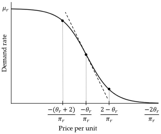
Figure 1.
Logit demand curve (reverse S-shaped).
In order to make the finished products, the manufacturer needs a set of raw materials and parts, denoted by . An item in may be used for making several finished products in . Let be the number of units of item required to make a single unit of finished product . The demand rate of item in iteration , denoted by , can be defined as follows:
In this study, we assume that shortages are not allowed for any member of the supply chain. The manufacturer cannot place orders that exceed the capacity rate of any supplier. However, the manufacturer can satisfy any demand rate determined by the demand response function as long as the required items are available. In addition, constant or negligible lead times are assumed.
In the proposed mechanism, suppliers use the flexible procurement CA bidding language in [36] to construct and submit their bids. Using this language, suppliers can offer multiple discount types, including synergy and all-unit quantity discounts. A synergy discount can be offered for bundles of items that have commonalities between them which reduce the supplier’s cost. Examples of these commonalities include similar raw materials, processing sequences, labor skills, etc. In addition, this language allows the manufacturer more freedom in selecting the order quantities and produces more efficient auction outcomes compared to other popular CA bidding languages. For the sake of completeness, we provide a brief description of the utilized bidding language.
Let be the set of bids submitted by supplier in iteration . is the set of items offered in bid . A flexible bid, , consists of a set of linear price functions, denoted by , that defines different prices for the items offered in the bid at different levels of purchase quantities. To be specific, each function defines a price per unit, denoted by , for every item , and a lower purchase quantity bound, denoted by . A price function can be used to determine the price of a package only if the order quantities of all items in exceed the associated lower bounds. The order quantity of item from bid offered by supplier in iteration is denoted by . For convenience of notation, from now on we drop the iteration index, , and add it only when referring to an iteration other than the current one. Mathematically, a bid is defined as follows:
where is the capacity per time unit of supplier for making item . Since purchase quantities can exceed the lower bounds of several functions in , we use the highest-ranking price function (lowest prices) with all quantity lower bounds exceeded. The only upper limit on the quantities ordered from any supplier is the supplier’s capacity rate . Figure 2 shows two flexible procurement CA bids submitted by supplier . It is important to note that in this bidding language, the manufacturer can select multiple bids from any participating supplier.
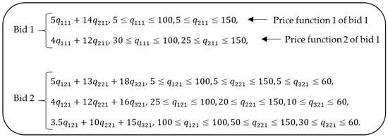
Figure 2.
Flexible procurement CA bidding language [36].
We use the term supplier’s true valuations to refer to the minimum prices that the supplier is willing to accept for the items in a certain bid and price function. The goal of the proposed mechanism is to maximize the manufacturer’s profit by disclosing the suppliers’ true valuations of the items offered in their submitted bids. This is achieved through multiple rounds of bidding, winner determination, and bid adjustments.
4. Methodology
The proposed auction mechanism iterates between the manufacturer and the suppliers. The manufacturer issues a request for bids from a set of pre-approved suppliers . These suppliers meet the minimum requirements of the manufacturer’s selection criteria, including economic stability, quality metrics, geographic location, communication systems, sustainability metrics, etc. Therefore, the winner determination is based on the manufacturer’s profit. The suppliers submit their initial bids. We assume that the initial bids are constructed outside the scope of this study. However, the items offered in each bid should have commonalities that help the supplier achieve higher production efficiency and cost reduction. The initial prices can be based on the supplier’s cost and market research [90,91,92].
The manufacturer solves a winner-determination problem to select suppliers, allocate order quantities, determine the selling prices of the finished products, and find the maximum profit that can be achieved given the submitted bids. The manufacturer stores the solution as well as the submitted bids in a database and makes it accessible to all suppliers. These data provide the suppliers with feedback to adjust their bids for the new iteration.
We assume that the combinations of items and lower order-quantity bounds in the initial bids are fixed. However, suppliers can adjust their selling prices to make their bids more attractive in the next iteration. The manufacturer asks any supplier planning to submit updated bids to adjust the selling prices and allow the manufacturer’s profit to increase by a certain profit-improvement factor. Given that the manufacturer’s profit in the current iteration is optimal under existing bids, a supplier cannot satisfy this constraint except by reducing his/her selling prices. This constraint guarantees the finiteness of the mechanism and convergence toward the suppliers’ minimum acceptable prices. This study considers a wide variety of procurement costs represented by realistic linear and non-linear formulas and continuous and discrete (integer) variables. Therefore, we developed an MINLP model to help the suppliers adjust their bids. The objective of the supplier’s model is to maximize the supplier’s expected profit while satisfying the manufacturer’s profit-improvement constraint. Each supplier solves the MINLP model assuming that the bids of the other suppliers will stay the same. If there is an optimal solution that improves the supplier’s profit, then he/she submits updated bids for the next iteration. Otherwise, the supplier does not submit updated bids. If none of the suppliers can find a feasible solution that satisfies both the manufacturer’s profit-improvement constraint and the supplier’s minimum desired profit markup, the manufacturer reduces the profit-improvement factor. The mechanism continues until no new updated bids are submitted and the manufacturer’s profit-improvement factor drops below a pre-determined minimum threshold.
Section 4.1 presents the manufacturer’s subproblem and uses the mathematical model in [36] to determine the winning bids. This section is included here for the sake of completeness. Section 4.2 discusses the supplier’s subproblem and proposed mathematical model. Finally, Section 4.3 discusses the overall mechanism and presents the auction algorithm.
4.1. The Manufacturer’s Subproblem
In the proposed mechanism, the manufacturer acts as an auctioneer. His/her role includes receiving and storing the submitted bids, solving the SSOA problem, updating the profit-improvement factor, and sharing information with the suppliers. In this section, we present the manufacturer’s mathematical model. This model is unique because it is based on an efficient flexible procurement CA bidding language, assumes price-sensitive demand rates for the finished products, and considers multiple types of costs that usually co-exist in practice. The manufacturer aims to maximize his/her earned profit, denoted by , from selling the finished products. To calculate this profit, we consider the earned revenue as well as the costs of purchasing, transportation, administration, order placement, and inventory holding. The formula that captures the manufacturer’s revenue per time unit, denoted by , is as follows:
The manufacturer’s purchasing cost is calculated based on the selected suppliers, bids, and price functions as well as the allocated order quantities. At the current iteration, let be the cycle time, is the number of orders per cycle time from supplier , and is a binary variable that takes the value 1 if the price function from bid offered by supplier is selected, and 0 otherwise. The formula for calculating the total purchasing cost per time unit, denoted by , is as follows:
Next, every time a new order is placed by the manufacturer to a supplier, an order placement cost is incurred. At the current iteration, let be a binary variable that takes the value 1 if supplier is selected, and 0 otherwise; is the cost to place one order from supplier . The formula for calculating the total ordering cost per time unit, denoted by , is as follows:
The administrative cost is the cost incurred by the manufacturer to maintain the relationship with the selected suppliers. This could include the cost of keeping records, on-site visits, maintaining communication systems, etc. The formula for calculating the total administrative cost per time unit, denoted by , is as follows:
where is the administrative cost per time unit to maintain the relationship with supplier .
To calculate the transportation cost, we consider one truck size with a weight capacity denoted by . However, the manufacturer can pay a fixed cost per truck shipped from supplier using the full TL rate, denoted by , or pay per weight unit using the LTL rate, denoted by . In practice, it is normal to have ; therefore, the manufacturer may prefer to pay the TL rate even if the shipment weight is less than the full truck capacity. Let be the weight per unit of item . Then, let be the number of full TL shipments from supplier . Also, let be a binary variable that takes the value 1 if it is cheaper to pay the full TL rate, , than to carry the remaining items which do not fill an entire truck, ; otherwise, . The formula for calculating the total transportation cost per time unit, denoted by , is as follows:
Note that the costs are divided by the cycle time in Equations (6), (7) and (9) to find the cost per time unit. For simplicity, let us define as the reciprocal of , .
Next, to simplify the calculation of the inventory holding cost, the following assumption is added:
- The demand rate of each item is distributed among the suppliers of the item proportionally. Mathematically, let be the part of the demand rate for item in the current iteration satisfied by supplier . Then, can be calculated as follows:
This assumption ensures that the quantity ordered from each supplier is consumed exactly before the following order from this supplier is placed. To illustrate this assumption, consider an example with one item purchased from two different suppliers. Let the demand rate of item be and the cycle time be . Then, let the order quantities be and and the order frequencies be and for suppliers 1 and 2, respectively. Figure 3 shows the demand rates and stock level patterns for this example under the added assumption.
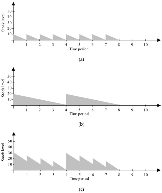
Figure 3.
Inventory level patterns. (a) Inventory level of item purchased from supplier , , . (b) Inventory level of item purchased from supplier , , . (c) Combined inventory level pattern of item at the manufacturer’s warehouse.
To calculate the inventory holding cost per time unit, denoted by , let be the holding cost of one unit of item per time unit. The formula for calculating is as follows:
The buyer’s model can be written as follows:
subject to
The objective function in Equation (12) maximizes the total manufacturer’s profit. Equations (13) and (14) define the demand rates of the finished products in and the items in . Constraint set (15) ensures that the manufacturer buys enough units to satisfy the demand rate for all items in . Constraint set (16) guarantees that order quantities exceed the lower quantity bounds for the selected price functions. Constraint set (17) makes sure that, at most, one price function is selected from each submitted bid. Constraint set (18) validates that when placing an order for a particular bid, a price function from this bid must be selected. Constraint set (19) verifies that the capacity rate of any item purchased from selected suppliers is not exceeded. Constraint sets (20) and (21) define the number of full TLs used to ship items from the selected suppliers to the manufacturer. Finally, (22) is the set of domain constraints.
4.2. The Supplier’s Subproblem
After solving the buyer’s model, the manufacturer shares the optimal solution with the suppliers, including the manufacturer’s profit, selected suppliers, and order allocation. Next, suppliers use this information, along with the most recent set of submitted bids, as feedback to improve their bids for the new auction iteration. However, the manufacturer asks any supplier planning to update his/her bids to adjust the selling prices in order to allow for an increase in the manufacturer’s profit by a given improvement factor. In this section, we develop a mathematical model for the suppliers to adjust their bids with the objective of maximizing their own expected profits while satisfying the auction mechanism rules and the imposed manufacturer’s profit-improvement constraint. Each supplier solves the model in every iteration under the assumption that the bids of the other suppliers stay the same.
We assume that the combinations of items and quantity bounds are fixed in all bids throughout the auction. However, the suppliers have the ability to adjust their selling prices. On the one hand, offering low prices increases the probability of a supplier being selected; however, profit margins may be too low to earn an acceptable profit. On the other hand, high prices may be associated with high profit margins; however, if the prices are too high, the bid may be unattractive, leading to the supplier missing out on a potential sale. Therefore, in an iterative auction mechanism, suppliers receive additional information after every iteration to guide their bid adjustments. The information-sharing rules are different from one auction design to another. In this study, we assume partial information sharing. The manufacturer receives the bids and stores them in a database accessible by all participating suppliers. This assumption benefits both the manufacturer and the suppliers. From the manufacturer’s perspective, sharing information can increase the competition and encourage the suppliers to lower their prices in order to win the auction. From the supplier’s perspective, access to the manufacturer’s database helps them to make informed pricing decisions and prevents unnecessary price cuts. However, suppliers do not share their costs and desired profit markups.
Internally, suppliers need to understand their cost structure in order to offer the best bids and be selected. Here, we discuss two possible discount types offered by the suppliers. The first discount type is the synergy or complementarity discount. This discount encourages the buyer to order a combination of items that are related or have common factors. These factors include similar raw materials, processing equipment, etc. Complementarities between items can lead to cost savings for the supplier. These savings give the supplier more room to lower selling prices and submit attractive bids. The value of the synergy discount can be different depending on the specific common factor, number of different items in the bid, different combinations of items, etc. We assume that suppliers consider this complementarity effect when choosing the items that go into each bid. The second discount type is an all-unit quantity discount. In general, suppliers benefit from economies of scale and experience a lower cost per unit for large orders. Therefore, within the same bid, a higher-ranking price function with higher values for the lower quantity bounds, , has lower unit prices. We assume that these two discount types are included by the supplier at the time of bid construction. Other discount types can be easily integrated into the proposed model by calculating their effect on the supplier’s costs and then allowing the supplier to drop the selling prices accordingly.
Let be the cost of item according to the price function of bid offered by supplier . We assume that every supplier has a minimum desired profit. Some studies refer to the profit that a business missed out on when choosing to pursue a business venture over another as the opportunity cost, arguing that if the supplier does not sell to a particular buyer, the supplier can use his/her capacity to make and sell items somewhere else, making this minimum profit [7,93]. The minimum profit can be defined in several ways. The first one is simply having a fixed profit value that supplier must earn to stay in the auction. Let this value be denoted by . The following constraint represents this definition:
This method does not take the size of the order or the supplier’s investment into account when calculating the minimum desired profit. The fixed desired profit, , can be too high considering the quantity/cost of items sold. Therefore, to satisfy constraint (23) the supplier’s selling prices have to be unreasonably high. Also, it may be the case that the quantity/cost of items sold is large, which makes the fixed value of relatively small and unattractive to the supplier. In addition, the supplier does not know what the actual order quantities will be at the time of constructing or updating the bids. Therefore, it is possible that the supplier sets the selling prices low and hopes to achieve profit based on high sales expectations. However, if the order quantities are lower than expected, the supplier will not achieve the minimum desired profit. Alternatively, if the sales forecast is too low, the supplier will ask for higher prices, and his/her bids may not be competitive. Mansouri and Hassini [33] discuss this problem, then propose a solution by making assumptions regarding the supplier’s risk tolerance.
In this study, we define the minimum desired profit as a percentage of the cost of items sold by the supplier. Let be the minimum acceptable profit markup, , where profit markup is defined as follows:
Therefore, the true valuation of item in bid and price function to supplier can be defined as . The following constraint ensures that the selling price of each item offered by supplier achieves the minimum profit markup:
Another alternative constraint could be to guarantee a minimum profit markup for the entire sale as follows:
An important aspect of the iterative auction mechanism design is its ability to progress and improve its outcomes over iterations. An iterative auction mechanism could get stuck before reaching a high-quality solution. This can happen if there are several suppliers offering similar prices and there are alternative optimal solutions to the buyer’s model. In this case, a mathematical model with the objective of maximizing the supplier’s expected profit will simply reallocate the orders without updating the selling prices. If this happens, the mechanism cannot disclose more information about the suppliers’ true valuations, and the manufacturer cannot make the most efficient purchasing decisions. Therefore, to move the auction mechanism forward, some studies define a minimum improvement that the bidder has to make in every iteration in order to stay in the auction. This is referred to as the improvement margin requirement [63]. Since we are considering a procurement CA with packages of items, suppliers may be able to reduce the prices of some items more than others. Also, if the supplier is already offering good prices and getting selected by the manufacturer, it is unreasonable to force this supplier to reduce the selling prices. Therefore, we propose that the manufacturer demand an increase in his/her profit by a given percentage, called the profit-improvement factor, from any supplier submitting an updated bid in the new iteration. Let the profit-improvement factor in the current iteration be denoted by .
Let be the expected profit of supplier in the current iteration. The supplier’s mathematical model is shown below. Keep in mind that each supplier solves this model assuming that none of the other suppliers update their bids. Note that this model uses similar parameters and decision variables as the buyer’s model. However, the prices, , offered by the supplier solving the model are now considered as decision variables, and we add the parameters and .
subject to
in addition to (13)–(22).
The objective function in Equation (27) maximizes the expected profit of supplier . Constraint (28) ensures that the manufacturer’s profit increases by at least over the profit of the previous iteration. Constraint set (29) ensures that the supplier achieves the desired minimum profit markup for every item sold. Constraint set (30) ensures that the selling prices in the supplier’s bids are greater than or equal to zero. Finally, constraints (13)–(22) enable the supplier to use the most recent bids shared by the manufacturer in his/her optimal solution.
Solving the supplier’s model in Equations (13)–(22) and (27)–(30) will not only adjust the selling prices but will also provide the supplier with a forecast regarding which suppliers, bids, and price functions will be selected. The supplier submits his/her updated bids that were selected in the supplier’s model solution.
Lemma 1.
A supplier, , solving the supplier’s model, will always reduce the selling prices of some items in the updated bids. In addition, if none of the other suppliers updates his/her bids, supplier is guaranteed to be selected in the new iteration.
Proof of Lemma 1.
The manufacturer’s profit in the previous iteration, , is optimal under the submitted bids. Given that supplier solves the supplier’s model assuming that the bids submitted by the other suppliers will stay the same, then the only way for supplier to improve the manufacturer’s profit and satisfy constraint (28) is to reduce the selling prices of some items in his/her updated bids. Next, the manufacturer solves the buyer’s model in the new iteration. Given the updated bids submitted by supplier , the profit is no longer optimal. If none of the other suppliers submitted updated bids, then the only way for the manufacturer to improve his/her profit is by selecting some of the updated bids submitted by supplier . □
Note that this mechanism gives the suppliers access to the demand functions of the finished products and their parameters. Therefore, the supplier’s model enables the supplier to anticipate the finished products’ selling prices and demands and then adjust the submitted bids in order to increase the profit of both the supplier and the manufacturer.
4.3. Auction Mechanism
The first iteration of the proposed auction mechanism starts with initial bids submitted by the suppliers to the manufacturer. The manufacturer stores these bids, along with the parameters of the demand functions of the finished products, in a database accessible to all participating suppliers. Suppliers keep their costs, , and profit markups, , as private information. The manufacturer solves the buyer’s model in Equations (12)–(22), which gives the optimal supplier selection, order allocation, cycle time, order frequency, transportation, and pricing decisions, given the submitted bids. After that, the manufacturer shares the optimal solution and the profit-improvement factor with the suppliers.
Note that each supplier can calculate his/her actual profit based on the manufacturer’s solution. Let us denote this profit by . If a supplier is not selected, then the profit of this supplier in the current iteration . Each supplier, , solves the model in Equations (13)–(22) and (27)–(30), assuming that none of the bids submitted by the other suppliers will change. If there is an optimal solution with a maximum profit, , that exceeds the actual profit earned by this supplier in the previous iteration, , then the supplier adjusts the selling prices and submits the updated bids. Otherwise, this supplier does not submit updated bids. Note that although suppliers have to reduce their selling prices in the updated bids, selected suppliers may still want to update their bids. This can happen if a selected supplier is allocated certain order quantities; however, the supplier expects to sell larger quantities and gain higher profit by reducing his/her selling prices. Alternatively, this can occur if the supplier is selected to provide a certain set of items, but he/she wants to compete to sell another set or obtain another bid selected. Based on this, suppliers do not submit updated bids in two cases:
- The supplier cannot find a feasible solution that satisfies the required improvement in the manufacturer’s profit, constraint (28), while maintaining the desired minimum profit markups, constraint (29).
- The profit of the optimal solution of the supplier’s model, , does not exceed the supplier’s actual profit from the optimal solution of the buyer’s model in the previous iteration, .
Note that since the supplier’s model is solved by each individual supplier under the assumption that none of the bids submitted by the other suppliers is updated, then in order to satisfy constraint (28), a supplier must reduce the selling prices in his/her updated bids (Lemma 1). Therefore, case 1 happens if the selling prices of the supplier are close to the true valuations. Therefore, the supplier cannot give the manufacturer the required profit improvement under the current value of and, at the same time, maintain the desired minimum profit markup. It may be worth mentioning here that larger packages with more items and higher quantity bounds can help the supplier distribute the price reduction and keep updating bids for more iterations. In case 2, the supplier finds an optimal solution that satisfies all the constraints in the supplier’s model. However, due to price reduction, the profit of this solution is less than the supplier’s actual profit based on the buyer’s decisions in the previous iteration, . Therefore, the supplier chooses not to submit updated bids.
The value of the manufacturer’s profit-improvement factor, , enables the manufacturer to control the pace of the auction mechanism. If is fixed for all iterations and the value is large, suppliers need to drop their prices quickly. This will accelerate the auction mechanism and reduce the number of iterations and computational effort. However, suppliers may stop updating their bids too early due to case 1 condition even though the gap between their current prices and their true valuations is still large. This will prevent the manufacturer from disclosing the true valuations of the suppliers, and he/she will have to buy from the suppliers at higher prices than what they can offer. On the other hand, if is fixed for all iterations and its value is small, suppliers will make small adjustments to their selling prices. Eventually, these adjustments will stop when some or all suppliers cannot afford to reduce their selling prices anymore, as in case 1. This will help the manufacturer get close to the suppliers’ true valuations; however, it will increase the number of iterations of the auction mechanism and the required computational effort.
Based on that, we propose to start at a relatively high value and then decrease it later in the auction mechanism. This allows the mechanism to move quickly at the beginning when suppliers have room for price adjustments, then move slower toward the end of the auction. This way, the auction can be efficient with a relatively small number of iterations, and the manufacturer knows that the selling prices at the end of the auction are reasonably close to the true valuations of the suppliers. The value of will not be reduced in every iteration; rather, we propose fixing the value of until we reach an iteration where none of the suppliers submits an updated bid. Let this iteration be . Now, the manufacturer multiplies by a reduction factor, denoted by , where .
After reducing , some suppliers may become able to update their bids. The mechanism continues, and gets updated every time no new bids are submitted until its value drops below a predetermined minimum level, denoted by . At this point, the auction terminates and the final solution is the optimal solution of the buyer’s model from the last iteration with updated bids. The buyer’s profit in the final solution is denoted by . The algorithm below summarizes the proposed iterative auction mechanism (Algorithm 1).
| Algorithm 1: Procurement CA Algorithm |
|
|
|
|
|
Figure 4 summarizes the proposed algorithm in a flowchart.
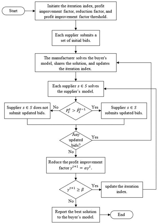
Figure 4.
Procurement CA algorithm flowchart.
Lemma 2 below indicates that this algorithm is finite and progresses toward disclosing the suppliers’ true valuations. This is important, especially if this algorithm is going to be used in an autonomous decision-making process.
Lemma 2.
The proposed procurement CA algorithm is finite.
Proof of Lemma 2.
There are two cases that affect the number of iterations in the proposed algorithm:
- 1.
- There are no new updated bids submitted; the algorithm iterates while updating the profit-improvement factor .
- 2.
- There are new updated bids submitted; the algorithm iterates without updating .
We need to prove that the total number of iterations in the two cases is finite.
Let be the number of times the manufacturer’s profit-improvement factor needs to be updated, multiplied by , to go from its initial value until it drops below the algorithm’s termination threshold . can be calculated as follows:
since , then
The number of iterations required until drops below for the first time is
Given that , , and , then the number of updates to in the proposed algorithm is finite.
Next, the algorithm can iterate without updating the value of as long as there are new updated bids submitted by the suppliers. Given constraint (28) in the supplier’s model, if there are new updated bids, the manufacturer’s profit must increase. Let the value of the profit-improvement factor be starting from iteration . If there are new updated bids in the following iterations, the manufacturer’s profits in these iterations will be bounded from below by the following sequence: , , , ,
Note that, since , the difference between the manufacturer’s profits in the consecutive iterations is increasing. Based on Propositions 1 and 2 from Duan and Ventura [89], the manufacturer’s revenue associated with the logit demand response functions is bounded from above.
Given that the manufacturer’s costs are greater than or equal to zero, then this is an upper bound to the manufacturer’s profit too. Provided the value of the profit-improvement factor , the maximum number of improvements to the manufacturer’s profit starting from iteration , denoted by , can be found as follows:
Given that and for our application, then , which corresponds to the maximum number of iterations between updates, is finite. Therefore, the total number of iterations in the proposed algorithm is finite. □
5. Experimental Results
In this section, we demonstrate and test the proposed iterative auction mechanism by solving sets of numerical examples. The examples were solved on a Windows 10 PC with a 3.60 GHz Intel® Core™ i7 CPU and 16 GB of RAM. The auction mechanism was coded in GAMS 39.2.0 modeling language, and the models in Equations (12)–(22) and (27)–(30) were solved using the BARON solver. In Section 5.1, two sets of randomly generated problems are solved using the proposed methodology. We solve all problems using the same values for the profit-improvement factor, , the reduction factor, , and the termination threshold . In Section 5.2, we conduct a sensitivity analysis to explore the effect of changing the values of the problem parameters. In addition, we add a second termination criterion based on the number of iterations.
5.1. Randomly Generated Problems
In order to test the proposed mechanism, two problem sets were generated, as shown in Table 1. The problems in each set have similar size attributes.

Table 1.
Experimental problem sets.
For each problem, the combinations of items in the bids were selected randomly; however, we imposed the condition that each item is offered by at least two suppliers. The individual problem’s parameters were generated, as shown in Table 2.
Table 2.
Formulas and distributions used to generate the parameters for the test problems.
In addition, the parameters in Table 3 were set to fixed values.
Table 3.
Fixed-value parameters.
Next, we focus on one of the problems and provide the details of the solution to show the progress of the mechanism. After that, a summary of the overall results is provided. This problem has three suppliers; each supplier offers one bid with two price functions. The initial bids are shown in Table 4.
Table 4.
Initial bids.
The suppliers’ costs associated with each bid and price function are provided in Table 5.
Table 5.
Suppliers’ costs per unit.
Considering the initial bids in iteration , the buyer solves the model in Equations (12)–(22) to select suppliers, allocate orders, and find the optimal profit. In this solution, cycles per time unit, per unit of finished product 1, and per unit of finished product 2; the rest of the solution is shown in Table 6 and Table 7. The manufacturer’s profit is , while the suppliers’ actual profits are , , and .
Table 6.
Manufacturer’s problem solution considering the initial bids—part 1.
Table 7.
Manufacturer’s problem solution considering the initial bids—part 2.
Next, the initial bids are shared with the three suppliers, along with the solution and the value of the profit-improvement factor. Each supplier solves the supplier’s problem to maximize his/her profit while satisfying the manufacturer’s profit-improvement constraint. Supplier 1 was selected in the initial iteration and cannot find a solution that will improve his/her expected profit. Therefore, supplier 1 does not submit a new updated bid. For supplier 2, even though he/she was selected in the initial iteration, the solution to the supplier’s model showed that the profit of supplier 2 is expected to improve by reducing the selling prices and obtaining higher order quantities. Therefore, supplier 2 submits an updated bid. Also, supplier 3, who was not selected in the initial iteration, submits an updated bid. The bids for the new iteration are shown in Table 8.
Table 8.
Updated bids for iteration 1.
The auction mechanism continues between the buyer and the suppliers. Figure 5 shows the change in profit for the manufacturer and the suppliers with iterations. Note that the profit of a given supplier may go down to zero in some iterations; this indicates that the supplier was not selected in those iterations.
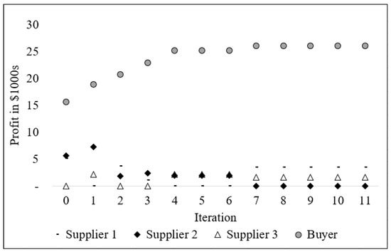
Figure 5.
Profit progress for the buyer and set of participating suppliers—problem 2.
Table 9 shows the profit-improvement factor and the selected suppliers in each iteration, as well as the associated change in profit for each auction participant. The auction took 11 iterations to terminate. The total CPU time to solve this example was 23,288.67 s, with an average time per iteration (including the initial iteration) of 1940.72 s. The profit of the buyer increased by compared to the buyer’s profit in the initial iteration. The sum of the suppliers’ profits decreased by .
Table 9.
Supplier selection and profit change through the auction mechanism.
To further assess the results, the true valuations of the suppliers were used as selling prices in the bids shown in Table 10. Solving the buyer’s model with the supplier’s true valuations as selling prices gives the highest possible profit that the buyer can achieve, denoted by . After that, we can compare with the best profit we were able to achieve using the proposed auction mechanism, .
Table 10.
True valuations of the suppliers used as selling prices (CPU time 597.08 s).
For our problem, the maximum possible profit , while our mechanism achieved . Therefore, the proposed methodology achieved of the maximum possible profit. This profit compares favorably with the percentage achieved in the initial iteration (single round auction), which was only of the maximum possible manufacturer’s profit. In addition, the selected suppliers, when using the suppliers’ true valuations, were suppliers 1 and 3, which are the same suppliers selected by the proposed methodology in the final iteration. However, based on the initial bids (single round auction), suppliers 1 and 2 were selected. Figure 6 shows the achieved profits as percentages of the maximum possible profits for the 10 problems described in Table 1. As can be seen in Figure 6, the iterative mechanism improved the manufacturer’s profit by as much as 118% in problem 5 of the first problem set.
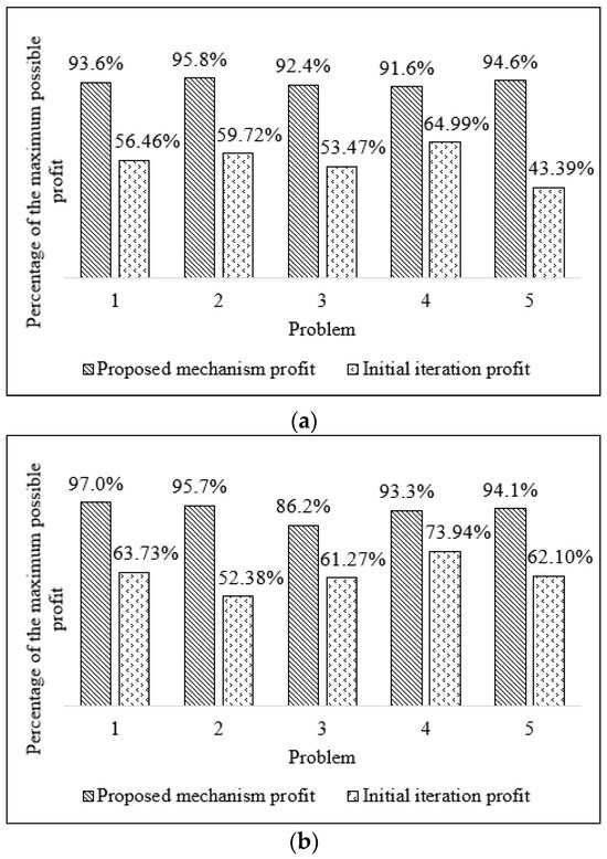
Figure 6.
Manufacturer’s profit at the end of the proposed mechanism versus profit of the initial iteration as percentages of the maximum possible profit for each problem. (a) Problem set 1. (b) Problem set 2.
Given the experimental results, we note that the auction outcomes are highly dependent on the level of competition between suppliers. If there is strong competition, i.e., the suppliers have similar costs and profit markups, then they will keep submitting updated bids and drive the selling prices down to be very close to their true valuations. However, if the costs and profit markups of some suppliers are significantly higher than the others, then these suppliers will stop bidding early in the process. Consequently, the other suppliers do not need to lower their prices to win the auction. This is expected in any iterative auction mechanism.
5.2. Discussion and Sensitivity Analysis
In this section, we discuss the effect of setting the mechanism parameters at different levels. A problem is solved using different sets of values for the mechanism parameters to show these effects.
An important factor to consider at the time of selecting the values of the mechanism parameters is the gap of lost improvement. This is the gap between the last value of before it drops below and the value of itself. In the previous section, the values of the parameters were , , and . Therefore, the last value of before it drops below is and the gap of lost improvement is . Hence, when the suppliers cannot afford to improve the manufacturer’s profit by , the auction ends, and the manufacturer will never know if any of the suppliers can afford an improvement between and . As can be seen, the values of the parameters were selected to have a small gap. However, if we set with the same values of and , the gap of lost improvement will increase to which may be significant depending on the application. The lowest gap can be achieved by setting the following:
where is an integer representing the number of updates to the profit-improvement factor.
As explained in the proof of Lemma 2, there are two types of iterations. In type 1 iterations, the algorithm iterates without new updated bids but changes the value of the profit-improvement factor , while in type 2 iterations, the algorithm iteratively updates bids but does not change the value of . The selection of the parameters’ initial values is a tradeoff between the number of type 1 and type 2 iterations. If the values of and were set to be relatively high and the value of was set to be small, in the beginning, the suppliers will need to improve the manufacturer’s profit significantly each time they update their bids. Thus, they will need to cut their selling prices quickly, and the number of iterations of the second type will be relatively small. However, the number of times needs to be updated will be relatively large. On the contrary, a small value of will allow the suppliers to make small adjustments to their bids, which increases the number of iterations between updates. The value of controls how quickly the mechanism goes from requiring the suppliers to make significant cuts to their selling prices to the case where they can make small adjustments to their bids.
In small-sized problems, where the computational effort is not a critical factor, the manufacturer should focus on selecting the parameter values to obtain a small gap of lost improvement. However, for larger-sized problems, where the computational effort is a critical factor, a second termination condition based on the number of iterations can be added. In this case, the parameter values should be selected to achieve the maximum possible profit improvement within the allowed number of iterations. If the manufacturer expects that the suppliers have room to reduce their prices, then he/she should select a high value for . However, if the suppliers cannot reduce their prices significantly, a high value of will increase the computational effort, and the algorithm will iterate without profit improvement. This can be seen in the following example.
Below, we use different sets of values for the mechanism parameters to solve the same problem explained in detail in the previous section. Here, we limit the number of iterations to 8. Table 11 shows a sample of the profit and CPU time data for these experiments.
Table 11.
Progress of the manufacturer’s profit with iterations using different values of and while keeping .
Figure 7 shows the progress of the manufacturer’s profit/week with iterations using different values for parameters and . As can be seen in Figure 7, setting to a high value helps improve the profit quickly in the beginning. This can be a good strategy if we are limited to a small number of iterations. Note that achieved the highest profit in two iterations. However, as the selling prices go down, suppliers will not be able to improve the manufacturer’s profit given the high value of . In addition, the high value of means that will be reduced slowly; therefore, the manufacturer needs to update the profit-improvement factor frequently. This can be seen between iterations 2 and 5 for the case where and in Figure 7. On the contrary, a low value for may not need to be updated frequently; however, it allows the suppliers to make minor adjustments, and the manufacturer’s profit will progress slowly. This may not be a good strategy for the manufacturer if the number of iterations is limited. The case where and achieved the highest profits for iterations 3 and above.
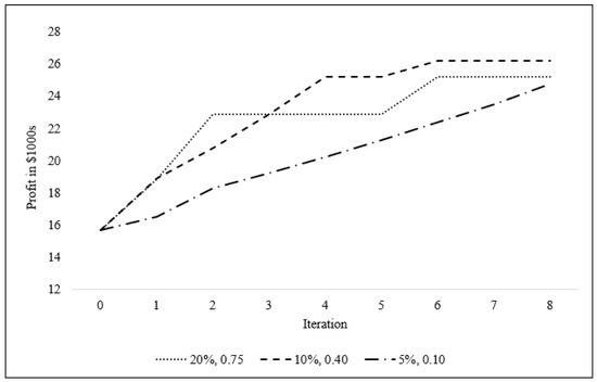
Figure 7.
Manufacturer’s profit/week progress with iterations given different values of and .
6. Conclusions and Future Research
In this study, we propose an iterative-procurement CA mechanism for the multi-item, multi-sourcing SSOA problem under a flexible bidding language. We assume that the demand rates of the finished products are price-sensitive following logit response functions. This study considers several types of procurement costs, including the costs of purchasing, transportation, order placement, administration, and inventory holding. These costs usually coexist in practice but are not always addressed together in research.
The mechanism starts with a set of initial bids submitted to the manufacturer. The manufacturer solves the buyer’s model in Equations (12)–(22) and shares the solution with the participating suppliers. Each supplier solves the model in (13)–(22) and (27)–(30). If there is an optimal solution with a higher expected profit compared to the supplier’s actual profit in the manufacturer’s solution from the previous iteration, the supplier submits a set of updated bids. Otherwise, the supplier does not update the existing bids. To progress toward the suppliers’ minimum acceptable selling prices and guarantee a finite number of auction iterations, we impose a manufacturer’s profit-improvement constraint on newly updated bids. This is achieved via a profit-improvement factor, , which ensures that suppliers reduce their selling prices in their updated bids. Eventually, some suppliers will not be able to submit newly updated bids while earning their desired minimum profit markup. We propose starting at a relatively high value to encourage suppliers to reduce their prices quickly. However, if no updated bids are submitted, is reduced using a reduction factor, , to allow the suppliers to find feasible solutions and submit updated bids. The value of controls how quickly the mechanism goes from demanding significant improvements to the manufacturer’s profit to the case where suppliers are making small adjustments. Eventually, will drop below the predetermined auction termination threshold, and the auction mechanism will stop.
The computational results show that in the case of a limited number of iterations, the manufacturer should pay more attention when setting the values of the mechanism parameters. The manufacturer should assess the submitted initial bids by comparing the selling prices with historical data, insights from market research, and experts’ opinions. If the manufacturer believes that the suppliers have plenty of room for reducing their prices, then he/she should select a relatively high initial value for the profit-improvement factor, . Otherwise, a smaller may be more appropriate to achieve the most profit improvement in the lowest number of iterations.
The experimental results show that the proposed mechanism can drive the selling prices close to the suppliers’ true valuations. However, the results depend on the level of competition in the auction. If the participating suppliers have similar costs and profit markups, they will continue to drop their prices until they are near their true valuations. However, if the costs and profit markups are significantly different, the suppliers with high costs and markups will stop bidding relatively early in the process. Consequently, the other suppliers have no incentive to update their bids and reduce their prices. This dependency on the level of competition is common among auction mechanisms.
Given that the main objective of the proposed methodology is to maximize the manufacturer’s profit considering revenue and procurement costs, the suppliers with lower costs of transportation, order placement, administration, and inventory holding, as well as better-selling prices, have a competitive advantage. Suppliers should not only focus on selling prices but also consider other costs paid by the buyer. For example, locating the supplier’s facilities near potential buyers reduces transportation costs and lead times. Investing in information technology and process improvement can make data exchange and communications with potential buyers easier and less costly. These investments can make suppliers more competitive and potentially more profitable in the long run.
Future research ideas include expanding the mathematical models to include sustainability criteria, considering stochastic price-sensitive demand rates of finished products, and assuming less information sharing in the mechanism. Lastly, the main limitation of the proposed methodology is the requirement to solve a combination of difficult problems. The computational effort for any realistically sized problem will be very high. Therefore, heuristic methods can be used to solve the mathematical models within the auction mechanism.
Author Contributions
Conceptualization, O.A. and J.A.V.; methodology, O.A.; software, O.A.; validation, O.A.; formal analysis, O.A.; investigation, O.A.; resources, O.A. and J.A.V.; writing—original draft preparation, O.A.; writing—review and editing, O.A. and J.A.V.; visualization, O.A.; supervision, J.A.V. All authors have read and agreed to the published version of the manuscript.
Funding
This research received no external funding.
Data Availability Statement
Data are contained within the article.
Conflicts of Interest
The authors declare no conflicts of interest.
References
- Beelen, C. Manage Product Complexity: How to Unlock Sales. Available online: https://www.xait.com/resources/blog/manage-product-complexity (accessed on 6 July 2024).
- Fürst, A.; Pecornik, N.; Hoyer, W.D. How Product Complexity Affects Consumer Adoption of New Products: The Role of Feature Heterogeneity and Interrelatedness. J. Acad. Mark. Sci. 2024, 52, 329–348. [Google Scholar] [CrossRef]
- Tang, Y.; Zhang, P. The Impact of Virtual Integration on Innovation Speed: On the View of Organizational Information Processing Theory. J. Organ. End User Comput. 2022, 34, 1–20. [Google Scholar] [CrossRef]
- Spina, G.; Caniato, F.; Luzzini, D.; Ronchi, S. Past, Present and Future Trends of Purchasing and Supply Management: An Extensive Literature Review. Ind. Mark. Manag. 2013, 42, 1202–1212. [Google Scholar] [CrossRef]
- Deng, S.; Xu, J. Manufacturing and Procurement Outsourcing Strategies of Competing Original Equipment Manufacturers. Eur. J. Oper. Res. 2023, 308, 884–896. [Google Scholar] [CrossRef]
- Magretta, J. The power of virtual integration: An interview with Dell Computer’s Michael Dell. Harvard Business Review, March–April 1998; pp. 73–84. [Google Scholar]
- Ventura, J.A.; Bunn, K.A.; Venegas, B.B.; Duan, L. A Coordination Mechanism for Supplier Selection and Order Quantity Allocation with Price-Sensitive Demand and Finite Production Rates. Int. J. Prod. Econ. 2021, 233, 108007. [Google Scholar] [CrossRef]
- Bhimani, A.; Ncube, M. Virtual Integration Costs and the Limits of Supply Chain Scalability. J. Account. Public Policy 2006, 25, 390–408. [Google Scholar] [CrossRef]
- Uygun, Y.; Gotsadze, N.; Schupp, F.; Gzirishvili, L.; Tindjou Nana, B.S. A Holistic Model for Understanding the Dynamics of Outsourcing. Int. J. Prod. Res. 2023, 61, 1202–1232. [Google Scholar] [CrossRef]
- Logistics Outsourcing Trends in 2020. Available online: https://www.gartner.com/smarterwithgartner/logistics-outsourcing-trends-in-2020 (accessed on 31 March 2022).
- Guchhait, R.; Sarkar, B. A Decision-Making Problem for Product Outsourcing with Flexible Production under a Global Supply Chain Management. Int. J. Prod. Econ. 2024, 272, 109230. [Google Scholar] [CrossRef]
- Koufteros, X.; Vickery, S.K.; Dröge, C. The Effects of Strategic Supplier Selection on Buyer Competitive Performance in Matched Domains: Does Supplier Integration Mediate the Relationships? J. Supply Chain Manag. 2012, 48, 93–115. [Google Scholar] [CrossRef]
- Ghadimi, P.; Toosi, F.G.; Heavey, C. A Multi-Agent Systems Approach for Sustainable Supplier Selection and Order Allocation in a Partnership Supply Chain. Eur. J. Oper. Res. 2018, 269, 286–301. [Google Scholar] [CrossRef]
- Yu, C.; Wong, T.N. An Agent-Based Negotiation Model for Supplier Selection of Multiple Products with Synergy Effect. Expert Syst. Appl. 2015, 42, 223–237. [Google Scholar] [CrossRef]
- Saputro, T.E.; Figueira, G.; Almada-Lobo, B. A Comprehensive Framework and Literature Review of Supplier Selection under Different Purchasing Strategies. Comput. Ind. Eng. 2022, 167, 108010. [Google Scholar] [CrossRef]
- Dertwinkel-Kalt, M.; Wey, C. Multi-Product Bargaining, Bundling, and Buyer Power. Econ. Lett. 2020, 188, 108936. [Google Scholar] [CrossRef]
- Parmigiani, A.; Mitchell, W. Complementarity, Capabilities, and the Boundaries of the Firm: The Impact of within-Firm and Interfirm Expertise on Concurrent Sourcing of Complementary Components. Strateg. Manag. J. 2009, 30, 1065–1091. [Google Scholar] [CrossRef]
- Zhang, Q.; Zheng, Y. Pricing Strategies for Bundled Products Considering Consumers’ Green Preference. J. Clean. Prod. 2022, 344, 130962. [Google Scholar] [CrossRef]
- Cramton, P.C.; Shoham, Y.; Steinberg, R. (Eds.) Combinatorial Auctions; MIT Press: Cambridge, MA, USA, 2006; ISBN 978-0-262-51413-2. [Google Scholar]
- Yang, F.; Li, S.; Huang, Y. The Bid Generation Problem in Combinatorial Auctions for Transportation Service Procurement. Int. J. Ind. Eng. Comput. 2023, 14, 511–522. [Google Scholar] [CrossRef]
- Palacios-Huerta, I.; Parkes, D.C.; Steinberg, R. Combinatorial Auctions in Practice. J. Econ. Lit. 2024, 62, 517–553. [Google Scholar] [CrossRef]
- Cardadeiro, E.; Gata, J. Scoring Auctions: Are They the Key to Marketbased Allocation of Airport Slots? Eur. Rev. Bus. Econ. 2021, 1, 59–76. [Google Scholar] [CrossRef]
- Kang, H.; Li, M.; Lin, L.; Fan, S.; Cai, W. Bridging Incentives and Dependencies: An Iterative Combinatorial Auction Approach to Dependency-Aware Offloading in Mobile Edge Computing. IEEE Trans. Mob. Comput. 2024, 1–18. [Google Scholar] [CrossRef]
- Gao, G.-X.; Han, M.; Li, X. Procurement of Last-Mile Delivery Capacity: A Reverse Auction Mechanism Considering Logistics Service Quality. Int. J. Logist. Res. Appl. 2024, 1–19. [Google Scholar] [CrossRef]
- Triki, C.; Piya, S.; Fu, L.-L. Integrating Production Scheduling and Transportation Procurement through Combinatorial Auctions. Networks 2020, 76, 147–163. [Google Scholar] [CrossRef]
- Bichler, M.; Shabalin, P.; Pikovsky, A. A Computational Analysis of Linear Price Iterative Combinatorial Auction Formats. Inf. Syst. Res. 2009, 20, 33–59. [Google Scholar] [CrossRef]
- Sen, A.K.; Bagchi, A.; Chakraborty, S. Designing Information Feedback for Bidders in Multi-Item Multi-Unit Combinatorial Auctions. Decis. Support Syst. 2020, 130, 113230. [Google Scholar] [CrossRef]
- Iftekhar, M.S.; Hailu, A.; Lindner, R.K. Does It Pay to Increase Competition in Combinatorial Conservation Auctions? Can. J. Agric. Econ. Can. Agroecon. 2014, 62, 411–433. [Google Scholar] [CrossRef]
- Milgrom, P.R.; Weber, R.J. A Theory of Auctions and Competitive Bidding. Econom. J. Econom. Soc. 1982, 50, 1089–1122. [Google Scholar] [CrossRef]
- Bichler, M.; Milgrom, P.; Schwarz, G. Taming the Communication and Computation Complexity of Combinatorial Auctions: The FUEL Bid Language. Manag. Sci. 2023, 69, 2217–2238. [Google Scholar] [CrossRef]
- Adomavicius, G.; Curley, S.P.; Gupta, A.; Sanyal, P. How Decision Complexity Affects Outcomes in Combinatorial Auctions. Prod. Oper. Manag. 2020, 29, 2579–2600. [Google Scholar] [CrossRef]
- De Vries, S.; Vohra, R.V. Combinatorial Auctions: A Survey. Inf. J. Comput. 2003, 15, 284–309. [Google Scholar] [CrossRef]
- Mansouri, B.; Hassini, E. Optimal Pricing in Iterative Flexible Combinatorial Procurement Auctions. Eur. J. Oper. Res. 2019, 277, 1083–1097. [Google Scholar] [CrossRef]
- Bichler, M.; Schneider, S.; Guler, K.; Sayal, M. Compact Bidding Languages and Supplier Selection for Markets with Economies of Scale and Scope. Eur. J. Oper. Res. 2011, 214, 67–77. [Google Scholar] [CrossRef]
- Phillips, R.L. Pricing and Revenue Optimization; Stanford University Press: Redwood City, CA, USA, 2021. [Google Scholar]
- Abbaas, O.; Ventura, J.A. A Flexible Combinatorial Auction Bidding Language for Supplier Selection and Order Allocation in a Supply Chain with Price Sensitive Demand. Comput. Ind. Eng. 2024, 194, 110373. [Google Scholar] [CrossRef]
- Manuel Maqueira, J.; Moyano-Fuentes, J.; Bruque, S. Drivers and Consequences of an Innovative Technology Assimilation in the Supply Chain: Cloud Computing and Supply Chain Integration. Int. J. Prod. Res. 2019, 57, 2083–2103. [Google Scholar] [CrossRef]
- Kumar, A.; Liu, R.; Shan, Z. Is Blockchain a Silver Bullet for Supply Chain Management? Technical Challenges and Research Opportunities. Decis. Sci. 2020, 51, 8–37. [Google Scholar] [CrossRef]
- Aissaoui, N.; Haouari, M.; Hassini, E. Supplier Selection and Order Lot Sizing Modeling: A Review. Comput. Oper. Res. 2007, 34, 3516–3540. [Google Scholar] [CrossRef]
- Di Pasquale, V.; Nenni, M.E.; Riemma, S. Order Allocation in Purchasing Management: A Review of State-of-the-Art Studies from a Supply Chain Perspective. Int. J. Prod. Res. 2020, 58, 4741–4766. [Google Scholar] [CrossRef]
- Aouadni, S.; Aouadni, I.; Rebaï, A. A Systematic Review on Supplier Selection and Order Allocation Problems. J. Ind. Eng. Int. 2019, 15, 267–289. [Google Scholar] [CrossRef]
- Rao, C.; Xiao, X.; Goh, M.; Zheng, J.; Wen, J. Compound Mechanism Design of Supplier Selection Based on Multi-Attribute Auction and Risk Management of Supply Chain. Comput. Ind. Eng. 2017, 105, 63–75. [Google Scholar] [CrossRef]
- Ghodsypour, S.H.; O’brien, C. A Decision Support System for Supplier Selection Using an Integrated Analytic Hierarchy Process and Linear Programming. Int. J. Prod. Econ. 1998, 56, 199–212. [Google Scholar] [CrossRef]
- Golmohammadi, D.; Mellat-Parast, M. Developing a Grey-Based Decision-Making Model for Supplier Selection. Int. J. Prod. Econ. 2012, 137, 191–200. [Google Scholar] [CrossRef]
- Ng, W.L. An Efficient and Simple Model for Multiple Criteria Supplier Selection Problem. Eur. J. Oper. Res. 2008, 186, 1059–1067. [Google Scholar] [CrossRef]
- Talluri, S.; Narasimhan, R. Vendor Evaluation with Performance Variability: A Max–Min Approach. Eur. J. Oper. Res. 2003, 146, 543–552. [Google Scholar] [CrossRef]
- Liang, D.; Li, Y.; Xin, J. Dynamic Selection and Order Allocation of Resilient Suppliers Based on Improved Fuzzy Multi-Criteria Decision Method. J. Chin. Inst. Eng. 2024, 47, 442–455. [Google Scholar] [CrossRef]
- Degraeve, Z.; Labro, E.; Roodhooft, F. An Evaluation of Vendor Selection Models from a Total Cost of Ownership Perspective. Eur. J. Oper. Res. 2000, 125, 34–58. [Google Scholar] [CrossRef]
- Alfares, H.K.; Turnadi, R. Lot Sizing and Supplier Selection with Multiple Items, Multiple Periods, Quantity Discounts, and Backordering. Comput. Ind. Eng. 2018, 116, 59–71. [Google Scholar] [CrossRef]
- Venegas, B.B.; Ventura, J.A. A Two-Stage Supply Chain Coordination Mechanism Considering Price Sensitive Demand and Quantity Discounts. Eur. J. Oper. Res. 2018, 264, 524–533. [Google Scholar] [CrossRef]
- Talluri, S. A Buyer–Seller Game Model for Selection and Negotiation of Purchasing Bids. Eur. J. Oper. Res. 2002, 143, 171–180. [Google Scholar] [CrossRef]
- Glickman, T.S.; White, S.C. Optimal Vendor Selection in a Multiproduct Supply Chain with Truckload Discounts. Transp. Res. Part E Logist. Transp. Rev. 2008, 44, 684–695. [Google Scholar] [CrossRef]
- Choudhary, D.; Shankar, R. Joint Decision of Procurement Lot-Size, Supplier Selection, and Carrier Selection. J. Purch. Supply Manag. 2013, 19, 16–26. [Google Scholar] [CrossRef]
- Ahmad, M.T.; Mondal, S. Dynamic Supplier Selection Model under Two-Echelon Supply Network. Expert Syst. Appl. 2016, 65, 255–270. [Google Scholar] [CrossRef]
- Gupta, S.; Ali, I.; Ahmed, A. Multi-Objective Bi-Level Supply Chain Network Order Allocation Problem under Fuzziness. Opsearch 2018, 55, 721–748. [Google Scholar] [CrossRef]
- Lo, H.-W.; Liou, J.J.; Wang, H.-S.; Tsai, Y.-S. An Integrated Model for Solving Problems in Green Supplier Selection and Order Allocation. J. Clean. Prod. 2018, 190, 339–352. [Google Scholar] [CrossRef]
- Vahidi, F.; Torabi, S.A.; Ramezankhani, M.J. Sustainable Supplier Selection and Order Allocation under Operational and Disruption Risks. J. Clean. Prod. 2018, 174, 1351–1365. [Google Scholar] [CrossRef]
- Saputro, T.E.; Figueira, G.; Almada-Lobo, B. Integrating Supplier Selection with Inventory Management under Supply Disruptions. Int. J. Prod. Res. 2021, 59, 3304–3322. [Google Scholar] [CrossRef]
- Luthra, S.; Govindan, K.; Kannan, D.; Mangla, S.K.; Garg, C.P. An Integrated Framework for Sustainable Supplier Selection and Evaluation in Supply Chains. J. Clean. Prod. 2017, 140, 1686–1698. [Google Scholar] [CrossRef]
- Hosseini, Z.S.; Flapper, S.D.; Pirayesh, M. Sustainable Supplier Selection and Order Allocation under Demand, Supplier Availability and Supplier Grading Uncertainties. Comput. Ind. Eng. 2022, 165, 107811. [Google Scholar] [CrossRef]
- Nayeri, S.; Khoei, M.A.; Rouhani-Tazangi, M.R.; GhanavatiNejad, M.; Rahmani, M.; Tirkolaee, E.B. A Data-Driven Model for Sustainable and Resilient Supplier Selection and Order Allocation Problem in a Responsive Supply Chain: A Case Study of Healthcare System. Eng. Appl. Artif. Intell. 2023, 124, 106511. [Google Scholar] [CrossRef]
- Wu, C.; Gao, J.; Barnes, D. Sustainable Partner Selection and Order Allocation for Strategic Items: An Integrated Multi-Stage Decision-Making Model. Int. J. Prod. Res. 2023, 61, 1076–1100. [Google Scholar] [CrossRef]
- Kelly, F.; Steinberg, R. A Combinatorial Auction with Multiple Winners for Universal Service. Manag. Sci. 2000, 46, 586–596. [Google Scholar] [CrossRef][Green Version]
- Pekeč, A.; Rothkopf, M.H. Combinatorial Auction Design. Manag. Sci. 2003, 49, 1485–1503. [Google Scholar] [CrossRef]
- Porter, D.; Rassenti, S.; Roopnarine, A.; Smith, V. Combinatorial Auction Design. Proc. Natl. Acad. Sci. USA 2003, 100, 11153–11157. [Google Scholar] [CrossRef]
- Kwon, R.H.; Anandalingam, G.; Ungar, L.H. Iterative Combinatorial Auctions with Bidder-Determined Combinations. Manag. Sci. 2005, 51, 407–418. [Google Scholar] [CrossRef]
- Dehghanbaghi, N.; Sajadieh, M.S. Joint Optimization of Production, Transportation and Pricing Policies of Complementary Products in a Supply Chain. Comput. Ind. Eng. 2017, 107, 150–157. [Google Scholar] [CrossRef]
- Alaei, R.; Setak, M. Selecting Unique Suppliers through Winner Determination in Combinatorial Reverse Auction: Scatter Search Algorithm. Sci. Iran. 2017, 24, 3297–3307. [Google Scholar] [CrossRef]
- Gujar, S.; Narahari, Y. Optimal Multi-Unit Combinatorial Auctions. Oper. Res. 2013, 13, 27–46. [Google Scholar] [CrossRef]
- Yu, C.; Wong, T.N. A Supplier Pre-Selection Model for Multiple Products with Synergy Effect. Int. J. Prod. Res. 2014, 52, 5206–5222. [Google Scholar] [CrossRef]
- Lopomo, G. The English Auction Is Optimal among Simple Sequential Auctions. J. Econ. Theory 1998, 82, 144–166. [Google Scholar] [CrossRef][Green Version]
- Brisset, K.; Cochard, F.; Le Gallo, J. Secret versus Public Reserve Price in an “Outcry” English Procurement Auction: Experimental Results. Int. J. Prod. Econ. 2015, 169, 285–298. [Google Scholar] [CrossRef]
- Sogn-Grundvåg, G.; Zhang, D.; Asche, F. Starting High or Low in English Auctions? The Case of Frozen Saithe in Norway. J. Agric. Appl. Econ. Assoc. 2024, 1–13. [Google Scholar] [CrossRef]
- Gonçalves, R.; Ray, I. Revenue Implications of Choosing Discrete Bid Levels in a Japanese–English Auction. Rev. Econ. Des. 2024, 28, 125–150. [Google Scholar] [CrossRef]
- Auster, S.; Kellner, C. Robust Bidding and Revenue in Descending Price Auctions. J. Econ. Theory 2022, 199, 105072. [Google Scholar] [CrossRef]
- Hafalir, I.; Luo, D.; Tao, C. Istanbul Flower Auction: The Need for Speed. arXiv 2024, arXiv:2404.08288. [Google Scholar]
- Mishra, D.; Parkes, D.C. Multi-Item Vickrey–Dutch Auctions. Games Econ. Behav. 2009, 66, 326–347. [Google Scholar] [CrossRef]
- Lai, M.; Cai, X.; Hu, Q. An Iterative Auction for Carrier Collaboration in Truckload Pickup and Delivery. Transp. Res. Part E Logist. Transp. Rev. 2017, 107, 60–80. [Google Scholar] [CrossRef]
- Kutanoglu, E.; David Wu, S. On Combinatorial Auction and Lagrangean Relaxation for Distributed Resource Scheduling. IIE Trans. 1999, 31, 813–826. [Google Scholar] [CrossRef]
- Mansouri, B.; Hassini, E. A Lagrangian Approach to the Winner Determination Problem in Iterative Combinatorial Reverse Auctions. Eur. J. Oper. Res. 2015, 244, 565–575. [Google Scholar] [CrossRef]
- Hsieh, F.-S. Combinatorial Reverse Auction Based on Revelation of Lagrangian Multipliers. Decis. Support Syst. 2010, 48, 323–330. [Google Scholar] [CrossRef]
- Goeree, J.K.; Holt, C.A.; Ledyard, J.O. An Experimental Comparison of the FCC’s Combinatorial and Non-Combinatorial Simultaneous Multiple Round Auctions; Citeseer: Princeton, NJ, USA, 2006. [Google Scholar]
- Los, J.; Schulte, F.; Spaan, M.T.; Negenborn, R.R. The Value of Information Sharing for Platform-Based Collaborative Vehicle Routing. Transp. Res. Part E Logist. Transp. Rev. 2020, 141, 102011. [Google Scholar] [CrossRef]
- McClellan, A. Knowing Your Opponents: Information Disclosure and Auction Design. Games Econ. Behav. 2023, 140, 173–180. [Google Scholar] [CrossRef]
- Ma, Y.; Wang, N.; Che, A.; Huang, Y.; Xu, J. The Bullwhip Effect under Different Information-Sharing Settings: A Perspective on Price-Sensitive Demand That Incorporates Price Dynamics. Int. J. Prod. Res. 2013, 51, 3085–3116. [Google Scholar] [CrossRef]
- Adeinat, H.; Ventura, J.A. Determining the Retailer’s Replenishment Policy Considering Multiple Capacitated Suppliers and Price-Sensitive Demand. Eur. J. Oper. Res. 2015, 247, 83–92. [Google Scholar] [CrossRef]
- Feng, L.; Chan, Y.-L. Joint Pricing and Production Decisions for New Products with Learning Curve Effects under Upstream and Downstream Trade Credits. Eur. J. Oper. Res. 2019, 272, 905–913. [Google Scholar] [CrossRef]
- Hajdinjak, M. Functions with Linear Price Elasticity for Forecasting Demand and Supply. BE J. Theor. Econ. 2021, 21, 149–168. [Google Scholar] [CrossRef]
- Duan, L.; Ventura, J.A. Technical Note: A Joint Pricing, Supplier Selection, and Inventory Replenishment Model Using the Logit Demand Function*. Decis. Sci. 2021, 52, 512–534. [Google Scholar] [CrossRef]
- Cachon, G.P.; Lariviere, M.A. Supply Chain Coordination with Revenue-Sharing Contracts: Strengths and Limitations. Manag. Sci. 2005, 51, 30–44. [Google Scholar] [CrossRef]
- Ferreira, K.D.; Wu, D.D. An Integrated Product Planning Model for Pricing and Bundle Selection Using Markov Decision Processes and Data Envelope Analysis. Int. J. Prod. Econ. 2011, 134, 95–107. [Google Scholar] [CrossRef]
- Feng, L.; Wang, W.-C.; Teng, J.-T.; Cárdenas-Barrón, L.E. Pricing and Lot-Sizing Decision for Fresh Goods When Demand Depends on Unit Price, Displaying Stocks and Product Age under Generalized Payments. Eur. J. Oper. Res. 2022, 296, 940–952. [Google Scholar] [CrossRef]
- Mohammaditabar, D.; Ghodsypour, S.H.; Hafezalkotob, A. A Game Theoretic Analysis in Capacity-Constrained Supplier-Selection and Cooperation by Considering the Total Supply Chain Inventory Costs. Int. J. Prod. Econ. 2016, 181, 87–97. [Google Scholar] [CrossRef]


Disclaimer/Publisher’s Note: The statements, opinions and data contained in all publications are solely those of the individual author(s) and contributor(s) and not of MDPI and/or the editor(s). MDPI and/or the editor(s) disclaim responsibility for any injury to people or property resulting from any ideas, methods, instructions or products referred to in the content. |
© 2024 by the authors. Licensee MDPI, Basel, Switzerland. This article is an open access article distributed under the terms and conditions of the Creative Commons Attribution (CC BY) license (https://creativecommons.org/licenses/by/4.0/).