A Study on Effects of Species with the Adaptive Sex-Ratio on Bio-Community Based on Mechanism Analysis and ODE

Abstract

The species of the adaptive male–female sex ratio has different effects on the bio-community. This paper is aimed at figuring out these effects through mechanism analysis and Ordinary Differential Equation (ODE). Hence, the ODE environmental model is created by combining the Lotka–Volterra model, the interspecific model, and other external factors. The stability is used to characterize these effects. According to this model, effects on bio-community stability under different male–female sex ratios are roughly observed. By innovatively considering different living environments during the species’ lifecycle, the ODE environmental model is optimized, and the effects of different male–female sex ratios on the bio-community are further analyzed by phase-track maps and relative standard deviation. It is found that there are different findings and features in resource-rich and resource-scarce living environments during the lifecycle. Meanwhile, bio-communities in these two types of environments are in a stable state based on different male–female sex ratios. Based on these findings, directive opinions can be used to manage and help relevant bio-communities.

1. Introduction

In the animal kingdom, most of the species are basically male or female. Typically, species are born with an approximate male–female sex ratio of 1:1, while some species will not conform to this male–female sex ratio for other reasons, known as adaptive male–female sex-ratio changes [1]. This kind of species’ male–female sex ratio can vary according to the external environments, with growth rates in the larval stage determining whether they are male or female and the availability of food influencing the growth rate of the larvae. Usually, the male group has a different capacity for foraging compared to the female group; the adjustment of male–female sex ratios may produce significant and varied effects on the bio-community and environment. If the effects can be figured out, it is meaningful to help manage and maintain the stability of the relevant bio-communities.

Currently, there are some successful research results in this field. For example, Sun Mingjie et al. studied the iron metabolism mechanism of lamprey that has the mechanism of the adaptive male–female sex ratio [2]. In studying interspecies relationships, the Lotka–Volterra model with multiple additional factors is used to more accurately reflect real-world bio-community dynamics and stability compared to using the ordinary competition model alone [3]. Different competitions and dependencies within and between species are considered, so the necessitating modifications are added to the model [4]. However, what is ignored in the current successful research results is that the competitive abilities of individuals vary by sex, affecting the bio-community structure, so the effects of male–female sex-ratio differences on bio-community dynamics and stability are innovatively included in this paper. Zhang Qi’s research about male–female sex ratio leading to notable variations in competitive ability [5] further underscores the importance of considering competitive ability changes under different male–female sex ratios. The model in this paper also innovatively considers changes in the living environment throughout one species’ lifecycle, which is ignored by the previous studies. Additionally, because manual capturing is not a part of the regular natural bio-community, the manual factor is added to the model to enhance its realism in this paper. Regarding the quantitative analysis of system stability, there are various interpretative methods. For example, the phase-track map and its equilibrium point can show the speed at which a bio-community system stabilizes, transitioning from periodic oscillations to a stable state [6,7]. The relative standard deviation can be used to assess real-time stability based on fluctuation levels [8]. Each method has its advantages. These approaches are synthetically applied for a more comprehensive analysis of system stability in this paper.

The aim of this paper is to construct a model of the bio-community in which the species with the adaptive male–female sex ratio is found, using mechanism analysis and ODE to study the effects of adaptive male–female sex ratios on the bio-community in different living environments during this species’ lifecycle. What is thought-provoking is that lamprey is one of the typical species with an adaptive male–female sex ratio. Lamprey can change male–female sex ratios based on environments during its lifecycle. In some large lake habitats, lamprey is recognized as an opponent with significant (often negative) effects on the bio-community. For example, in the Great Lakes region of North America, the invasion of lamprey has had a significant effect on bio-communities [9]. At the same time, this species is treated as food by local people in other parts of the world [2]. These features are all in accord with the target species’ features in this paper. To better understand and implement the simulating and constructing processes, the lamprey is chosen to instance the species with the adaptive male–female sex ratio in the models of this paper. Meanwhile, a reasonable and necessary hypothesis is made as follows: in a bio-community, lamprey is a predator since lamprey attach to the body surface of fish and feed mainly on their blood and flesh, sometimes carrion [10]. Consequently, in this paper, the lamprey is treated as a predator. Based on this, the instantiation of this model is more reasonable.

Generally, based on the above analysis, the reviews of the existing research achievements and hypothesis, the main work of this paper is shown as follows:

(1)

Use mechanism analysis and the relevant ODE models to construct the ODE environmental model to simulate the evolution of the bio-community under one species’ different male–female sex ratios. This model consists of various factors, and the numerical solution actually means the densities of various species;

(2)

Given different living environments during one species’ lifecycle, the ODE environmental model is optimized. The relative standard deviation and the phase-track maps are chosen to explore the effects from the perspective of quantitative analysis;

(3)

Given different living environments in one species’ lifecycle, the ODE environmental model is optimized. The relative standard deviation and the phase-track map are chosen to explore the effects from the perspective of quantitative analysis;

(4)

Finally, putting lamprey in the optimal model, speeds at which equilibrium points in corresponding phase-track maps are reached and the values of the volatility depicted by relative standard deviation can be gained to compare the stability states of the bio-communities in different environments of lifecycle and the corresponding male–female sex-ratios of lamprey. Based on this, the effects can be figured out, and some problems in the relevant bio-communities can obtain some directive options.

2. The Construction of the ODE Environmental Model and Instantiation

The entire model construction mainly focuses on two original parts. First, this paper creates the ODE environmental model, which is used for qualitative analysis of the stability of the bio-community. Second, based on the ODE environmental model that is performed fundamentally, the optimal ODE environmental model is created to be used for the quantitative analysis of the stability of the bio-community. More details are as follows.

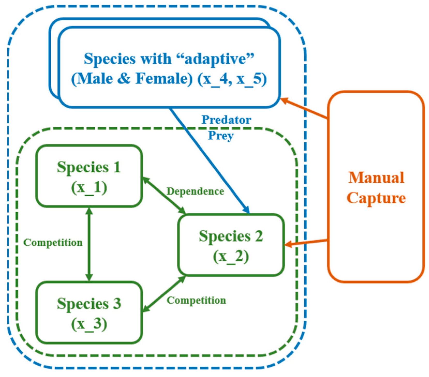
2.1. The Conception of the ODE Environmental Model

During the process of constructing this ODE model, it is critical to consider clearly the background of the bio-community [11] where the species with the adaptive male–female sex ratio can live. Consequently, in order to reduce the complexity of the model and make it easier to understand and implement while ensuring a comprehensive bio-community with as many interspecies relationships as possible, based on the purpose of studying the effects that may vary by sex, this paper sets five species in the ODE environment model, numbered 1–5. These species include the predator, its food bait, and other species, satisfying the interdependence and competition between different populations. The structure of the ODE environment model is shown in Figure 1.

Observation of the above figure shows that species 3 ($x_3$) and species 1, 2 ($x_{\mathrm{1,2}}$) are in competition with each other, and species 1 and 2 are interdependent. Meanwhile, species 4 and 5 ($x_{\mathrm{4,5}}$) are the male and female groups, respectively, of the species with the adaptive male–female sex ratio. The male and the female groups are divided into two separate species, which may be more convenient for reflecting the effects of different male–female sex ratios on the bio-community in the initial stage of constructing a model.

To better construct this model, key notations are summarized, as shown in

Table 1. Notations used in this paper.

Notation	Description
$i, j$	The species index
$x_i$	The density of species $i$
$N_i$	The environmental carrying capacity of species $i$
$D_i$	The binary variable showing whether it can survive on species $i$’s own
$r_i$	The intrinsic growth rate (mortality) of species $i$
$n_{ij}$	The binary variable showing the relationship between species $i$ and $j$
$R_i$	The relative standard deviation of species $i$
$\delta$	The male–female sex ratio coefficient
${\lambda }_{ij}$	The predation coefficient between species $i$ and j
${\lambda }_{ij}^{*}$	The combined predation coefficient between species $i$ and j
${\sigma }_{ij}$	The multiple of species $j$’s consumption of food relative to species $i$’s consumption of food

.

According to the above notation table, the ODE environmental model can be generated. Species 1 and species 3 are first analyzed, and the corresponding species’ evolutions are modeled. When only competition exists in the bio-community, a blocked growth model is given and shown in Equation (1):

$${\displaystyle \frac{dx(t)}{dt}}=rx(1-{\displaystyle \frac{x}{N}})$$

(1)

Based on this, for species 1 and species 3, let $x_1(t)$ and $x_3(t)$ be the density of the two species in the time dimension, $r_1$ and $r_3$ be the intrinsic growth rates of these two species, $N_1$ and $N_3$ be the environmental carrying capacity of these two species. When the effect of species 3 on species 1 is considered, $(x_3/N_3)$ should be subtracted. To reflect the difference in consumption between the two species, a factor ${\sigma }_{13}$ is set. The model of density-blocked growth of species 1 under competition from species 3, obtained from the above mechanism analysis, is shown in Equation (2)

$${\displaystyle \frac{d{x}_1(t)}{dt}}=r_1{x}_1(1-{\displaystyle \frac{x_1}{N_1}}-{\sigma }_{13}{\displaystyle \frac{x_3}{N_3}})$$

(2)

The model described above is based on the competition relationship. The model of density blocked growth for species 3 is similar, which is a conserved process of Equation (2). Given that there are also interdependencies in the bio-community, the interdependencies are discussed next. If species 1 has the ability to survive alone and species 2 does not have the ability to survive alone, species 2 will promote species 1’s development; according to Equation (1), the density of species 1 is defined again in Equation (3)

$${\displaystyle \frac{d{x}_1(t)}{dt}}=r_1{x}_1(1-{\displaystyle \frac{x_1}{N_1}}-{\sigma }_{13}{\displaystyle \frac{x_3}{N_3}}+{\sigma }_{12}{\displaystyle \frac{x_2}{N_2}})$$

(3)

Since species 2 cannot survive alone with $r_2$ as its mortality rate, it is now fed by species 1 that can survive alone. The density of species 2 $x_2(t)$ is Equation (4)

$${\displaystyle \frac{d{x}_2(t)}{dt}}=r_2{x}_2(-1+{\sigma }_{21}{\displaystyle \frac{x_1}{N_1}})$$

(4)

Over time, $({\sigma }_{21}{x}_1/N_1)$ will be greater than 1. When the density of species 2 is too large, it is necessary to add a blocking term to it, and the model of species 2 is Equation (5)

$${\displaystyle \frac{d{x}_2(t)}{dt}}=r_2{x}_2(-1-{\displaystyle \frac{x_2}{N_2}}+{\sigma }_{21}{\displaystyle \frac{x_1}{N_1}})$$

(5)

Species 2 is not able to survive alone, at which point the growth model obtained when both species 1 and species 2 are able to survive alone is as below:

$$\left\{ \begin{array}{c}{\displaystyle \frac{d{x}_1(t)}{dt}}=r_1{x}_1(1-{\displaystyle \frac{x_1}{N_1}}+{\sigma }_{12}{\displaystyle \frac{x_2}{N_2}})\\ {\displaystyle \frac{d{x}_2(t)}{dt}}=r_2{x}_2(1-{\displaystyle \frac{x_2}{N_2}}+{\sigma }_{21}{\displaystyle \frac{x_1}{N_1}})\end{array}\right.$$

(6)

There are also cases when neither species 1 nor species 2 can survive alone, which is in Equation (7)

$$\left\{ \begin{array}{c}{\displaystyle \frac{d{x}_1(t)}{dt}}=r_1{x}_1(-1-{\displaystyle \frac{x_1}{N_1}}+{\sigma }_{12}{\displaystyle \frac{x_2}{N_2}})\\ {\displaystyle \frac{d{x}_2(t)}{dt}}=r_2{x}_2(-1-{\displaystyle \frac{x_2}{N_2}}+{\sigma }_{21}{\displaystyle \frac{x_1}{N_1}})\end{array}\right.$$

(7)

Consequently, to combine competition and dependence, this paper innovatively proposes the coefficient $n_{ij}$ as a dichotomous variable for discrimination, which takes the value of “1” when there is competition and “−1” when there is a dependence. In the above analysis, the survival ability of the species itself is also involved. This paper introduces the coefficient $D_i$ to characterize whether the species can survive alone or not, which takes the value of “1” when it can survive alone and the value of “−1” when it cannot survive alone. In a competitive relationship, both competitors can survive alone by default. Details about the combining process are organized as shown in

Table 2. List of dichotomous variables for discrimination.

Variable Information	${\mathit{n}}_{\mathit{i}\mathit{j}}$		${\mathit{D}}_{\mathit{i}}$
Retrieve a value	1	−1	1	−1
Hidden meaning	competition	dependence	survive alone	unable to survive alone

.

Taking species 1 as an example, the coefficients are incorporated into the model to determine the growth of the species. The updated model is shown in Equation (8):

$${\displaystyle \frac{d{x}_1\left(t\right)}{d\left(t\right)}}=r_1{x}_1\left(D_1-{\displaystyle \frac{x_1}{N_1}}-n_{12}{\sigma }_{12}{\displaystyle \frac{x_2}{N_2}}-n_{13}{\sigma }_{13}{\displaystyle \frac{x_3}{N_3}}\right)$$

(8)

Based on Equation (8), the models of species 2 and species 3 are similar. The ODE environmental model, excluding the species with the adaptive male–female sex ratio and manual factors, can be constructed. This model can be used to observe the initial status as a control group, which is shown in Equation (9):

$$\left\{ \begin{array}{c}{\displaystyle \frac{d{x}_1\left(t\right)}{d\left(t\right)}}=r_1{x}_1\left(D_1-{\displaystyle \frac{x_1}{N_1}}-n_{12}{\sigma }_{12}{\displaystyle \frac{x_2}{N_2}}-n_{13}{\sigma }_{13}{\displaystyle \frac{x_3}{N_3}}\right)\\ {\displaystyle \frac{d{x}_2\left(t\right)}{d\left(t\right)}}=r_2{x}_2\left(D_2-{\displaystyle \frac{x_2}{N_2}}-n_{12}{\sigma }_{21}{\displaystyle \frac{x_1}{N_1}}-n_{23}{\sigma }_{23}{\displaystyle \frac{x_3}{N_3}}\right)\\ {\displaystyle \frac{d{x}_3\left(t\right)}{d\left(t\right)}}=r_3{x}_3\left(D_3-{\displaystyle \frac{x_3}{N_3}}-n_{13}{\sigma }_{31}{\displaystyle \frac{x_1}{N_1}}-n_{23}{\sigma }_{32}{\displaystyle \frac{x_2}{N_2}}\right)\end{array}\right.$$

(9)

In the bio-community, there is also a relationship between predator and prey, and the prey species is called food bait. Because this kind of species’ male–female sex ratio can be influenced by the availability of food, it is treated as a kind of predator in this paper. Species 2 is its food bait. Based on this fundamental precept, the following study is implemented.

First, the densities of the species with the adaptive male–female sex ratio and its food bait at the moment $t$ are denoted as $x_{\mathrm{4,5}}\left(t\right)$ and $x_2\left(t\right)$. It can be hypothesized that if the food bait can survive alone, the species with the adaptive male–female sex ratio will reduce the growth rate of food bait. Based on the Lotka–Volterra model to carve the predator-prey relationship [12], details are in Equation (10):

$${\displaystyle \frac{d{x}_2}{dt}}=x_2(r_2-{\lambda }_2{x}_{45})$$

(10)

where ${\lambda }_2$ is the predation coefficient of species 2, reflecting the ability of the special predator to catch this food bait. Similarly, what can be obtained is shown in Equation (11):

$${\displaystyle \frac{d{x}_{45}}{dt}}=x_{45}(-r_{45}+{\lambda }_{45}{x}_2)$$

(11)

where ${\lambda }_{45}$ is the predation coefficient of species 4 and species 5.

Equations (10) and (11) are in the absence of human intervention, but in real life, manual capturing cannot be ignored. Now, the manual capturing is added, and the intensity of manual capture is set as $e$. Currently, the growth rate of the food bait, species 2, slows down as $(r_2-e)$; the mortality rate of this predator increases as $(r_{45}+e)$. These changes are incorporated into the blocked growth model and shown in Equation (12)

$$\left\{ \begin{array}{l}{\displaystyle \frac{d{x}_2}{dt}}=x_2[(r_2-e)-{\lambda }_2{x}_{45}]\\ {\displaystyle \frac{d{x}_{45}}{dt}}=x_{45}[-(r_{45}+e)+{\lambda }_{45}{x}_2]\end{array}\right.$$

(12)

To combine the blocked growth model with the predation model and better portray the development trend of the species with the adaptive male–female sex ratio and its food bait, this paper preliminarily introduces $S_{\mathrm{1,2}}$ to individually describe the predator proportion of the current corresponding sex. Here, $S_1$ corresponds to the male group, and $S_2$ corresponds to the female group. These two coefficients $S_1$ and $S_2$ always add up to 1. Incorporating these coefficients into the blocked growth model developed above yields a development model for species 2, as shown in Equation (13):

$${\displaystyle \frac{d{x}_2\left(t\right)}{d\left(t\right)}}={(r}_2-e)x_2\left(D_2-{\displaystyle \frac{x_2}{N_2}}-n_{12}{\sigma }_{21}{\displaystyle \frac{x_1}{N_1}}-n_{23}{\sigma }_{23}{\displaystyle \frac{x_3}{N_3}}\right)-S_1{\lambda }_{24}{x}_2{x}_4-S_2{\lambda }_{25}{x}_2{x}_5$$

(13)

For species 4 and species 5, the relationship is intraspecific rather than interspecific because they are the same species, so other species have much greater effects on species 4 and 5. Then, the approximation of species 4 and 5 conforms to a mutually beneficial relationship, and by applying the blocked growth model of dependence, the densities of species 4 and species 5 can be expressed as shown in Equation (14):

$$\left\{ \begin{array}{c} {\displaystyle \frac{d{x}_4\left(t\right)}{d\left(t\right)}}=(r_4+e)x_4\left(D_4-{\displaystyle \frac{x_4}{N_4}}-n_{45}{\sigma }_{45}{\displaystyle \frac{x_5}{N_5}}\right)+{\lambda }_{42}{x}_4{x}_2\\ {\displaystyle \frac{d{x}_5\left(t\right)}{d\left(t\right)}}=(r_5+e)x_5\left(D_5-{\displaystyle \frac{x_5}{N_5}}-n_{45}{\sigma }_{54}{\displaystyle \frac{x_4}{N_4}}\right)+{\lambda }_{52}{x}_5{x}_2\end{array}\right.$$

(14)

According to Equation (14), and based on the development models of species 1, 2, and 3 established by Equations (9) and (13), the entire ODE environmental model can be integrated and defined as shown in Equation (15):

$$\begin{array}{l}{\displaystyle \frac{d{x}_1\left(t\right)}{d\left(t\right)}}=r_1{x}_1\left(D_1-{\displaystyle \frac{x_1}{N_1}}-n_{12}{\sigma }_{12}{\displaystyle \frac{x_2}{N_2}}-n_{13}{\sigma }_{13}{\displaystyle \frac{x_3}{N_3}}\right)\\ {\displaystyle \frac{d{x}_2\left(t\right)}{d\left(t\right)}}={(r}_2-e)x_2\left(D_2-{\displaystyle \frac{x_2}{N_2}}-n_{12}{\sigma }_{21}{\displaystyle \frac{x_1}{N_1}}-n_{23}{\sigma }_{23}{\displaystyle \frac{x_3}{N_3}}\right)-S_1{\lambda }_{24}{x}_2{x}_4-S_2{\lambda }_{25}{x}_2{x}_5\\ {\displaystyle \frac{d{x}_3\left(t\right)}{d\left(t\right)}}=r_3{x}_3\left(D_3-{\displaystyle \frac{x_3}{N_3}}-n_{13}{\sigma }_{31}{\displaystyle \frac{x_1}{N_1}}-n_{23}{\sigma }_{32}{\displaystyle \frac{x_2}{N_2}}\right)\\ \begin{array}{c}{\displaystyle \frac{d{x}_4\left(t\right)}{d\left(t\right)}}=(r_4+e)x_4\left(D_4-{\displaystyle \frac{x_4}{N_4}}-n_{45}{\sigma }_{45}{\displaystyle \frac{x_5}{N_5}}\right)+{\lambda }_{42}{x}_4{x}_2\\ {\displaystyle \frac{d{x}_5\left(t\right)}{d\left(t\right)}}=(r_5+e)x_5\left(D_5-{\displaystyle \frac{x_5}{N_5}}-n_{45}{\sigma }_{54}{\displaystyle \frac{x_4}{N_4}}\right)+{\lambda }_{52}{x}_5{x}_2\end{array}\end{array}$$

(15)

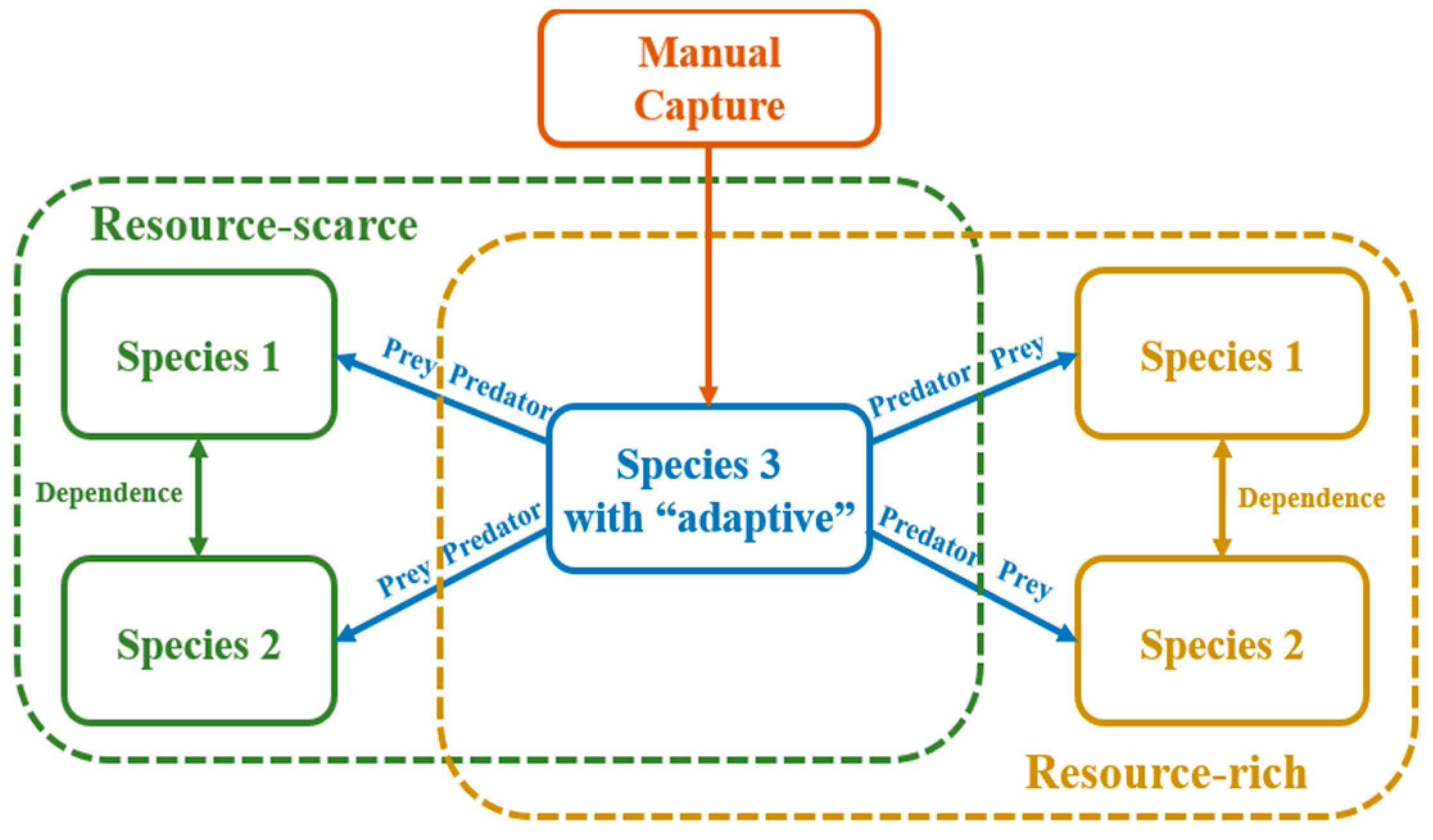
2.2. The Conception of the Optimal ODE Environmental Model

The current ODE environmental model is not perfect, even if there are some factors considered and innovation points, such as the manual factor. There are existing drawbacks. Firstly, it is indirect and redundant to use the predator proportion, $S_1$ and $S_2$, to reflect adaptive male–female sex ratios. Secondly, the male and the female groups are treated as two different species. This not only does not completely conform to the real situation but also increases the complexity of the model.

According to the above drawbacks, the optimal ODE environmental model should be implemented. Firstly, this paper introduces the definition of male–female sex-ratio coefficient and combines the predation coefficient to directly reflect the species’ different adaptive male–female sex ratios. Secondly, the male and the female groups are not divided into two species but are integrated into one species to better align with the actual situation. Thirdly, according to the lifecycle, different environmental carrying capacities are used for resource-scarce and resource-rich environments to optimize the current environmental model. Additionally, to simplify the model, making it clearer and easier to simulate and implement, only interspecies relations and species directly influenced by the species with adaptive male–female sex ratios are considered. Based on the above thoughts, a stable and reasonable bio-community can be better simulated, rather than having most species nearly extinct due to irrational interspecific relationships in the simulation. The detailed structure of the optimal one is shown in Figure 2.

Additionally, unlike qualitative analysis, the relative standard deviation and the phase-track maps are also defined to help analyze the stability of the entire bio-community under the effects of species 3’s different adaptive male–female sex ratios.

To more directly explore the effects of species 3’s change in male–female sex ratios on the bio-community, the male–female sex-ratio coefficient $\delta$ is introduced to represent the male–female sex ratio, allowing for a better understanding of species 3’s effects on the stability of the bio-community under its different male–female sex ratios.

In species 3, the male proportion is $a$, the female proportion is $(1-a)$, and the $\delta$ is $(1-a)/a$. Based on the above analysis and the predation coefficient ${\lambda }_{ij}$, to simplify and combine the male and female groups without affecting corresponding different predator abilities, the combined predation coefficient ${\lambda }_{ij}^{*}$ is defined and shown in Equation (16).

$${\lambda }_{ij}^{\mathrm{*}}=a({\displaystyle \frac{{\lambda }_{ij-male}}{\delta }}+{\lambda }_{ij-female})$$

(16)

As for the resource-scarce environment and the resource-rich environment, the simulation is realized by changing the environmental carrying capacity $N_i$ in different optimal ODE environmental models for different environments.

For species 3, manual capturing intensity $e$ also needs to be considered. Hence, the optimal ODE environmental model for the resource-scarce environment is shown in Equation (17):

$$\left\{ \begin{array}{l}{\displaystyle \frac{d{x}_1\left(t\right)}{d\left(t\right)}}=r_1{x}_1\left(D_1-{\displaystyle \frac{x_1}{N_1}}-n_{12}{\sigma }_{12}{\displaystyle \frac{x_2}{N_2}}\right)-\delta {\lambda }_{13}^{*}{x}_1{x}_3\\ {\displaystyle \frac{d{x}_2\left(t\right)}{d\left(t\right)}}=r_2{x}_2\left(D_2-{\displaystyle \frac{x_2}{N_2}}-n_{12}{\sigma }_{21}{\displaystyle \frac{x_1}{N_1}}\right)-\delta {\lambda }_{23}^{*}{x}_2{x}_3\\ {\displaystyle \frac{d{x}_3\left(t\right)}{d\left(t\right)}}={-(r}_3+e)x_3+\delta {\lambda }_{31}^{*}{x}_1{x}_3+\delta {\lambda }_{32}^{*}{x}_2{x}_3\end{array}\right.$$

(17)

Similarly, the optimal ODE environmental model for the resource-rich environment is shown in Equation (18):

$$\left\{ \begin{array}{l}{\displaystyle \frac{d{x}_1^{\prime }\left(t\right)}{d\left(t\right)}}=r_1{x}_1^{\prime }\left(D_1-{\displaystyle \frac{x_1^{\prime }}{N_1^{\prime }}}-n_{12}{\sigma }_{12}{\displaystyle \frac{x_1^{\prime }}{N_2^{\prime }}}\right)-\delta {\lambda }_{13}^{*}{x}_1^{\prime }{x}_3^{\prime }\\ {\displaystyle \frac{d{x}_2^{\prime }\left(t\right)}{d\left(t\right)}}=r_2{x}_2^{\prime }\left(D_2-{\displaystyle \frac{x_2^{\prime }}{N_2^{\prime }}}-n_{12}{\sigma }_{21}{\displaystyle \frac{x_1^{\prime }}{N_1^{\prime }}}\right)-\delta {\lambda }_{23}^{*}{x}_2^{\prime }{x}_3^{\prime }\\ {\displaystyle \frac{d{x}_3^{\prime }\left(t\right)}{d\left(t\right)}}={-(r}_3+e)x_3^{\prime }+\delta {\lambda }_{31}^{*}{x}_1^{\prime }{x}_3^{\prime }+\delta {\lambda }_{32}^{*}{x}_2^{\prime }{x}_3^{\prime }\end{array}\right.$$

(18)

Meanwhile, the relative standard deviation $R_i$ is introduced to help quantitatively analyze the stability of the bio-community under the effects of different adaptive male–female sex ratios, as shown in Equation (19):

$$R_i={\displaystyle \frac{\sqrt{\frac{\sum _{i=1}^n{(x_i-\overline{x})}^2}{n-1}}}{\overline{x}}}\times 100\%$$

(19)

When the relative standard deviation is smaller, it means that the volatility at this point is less, and the bio-community is more stable [13].

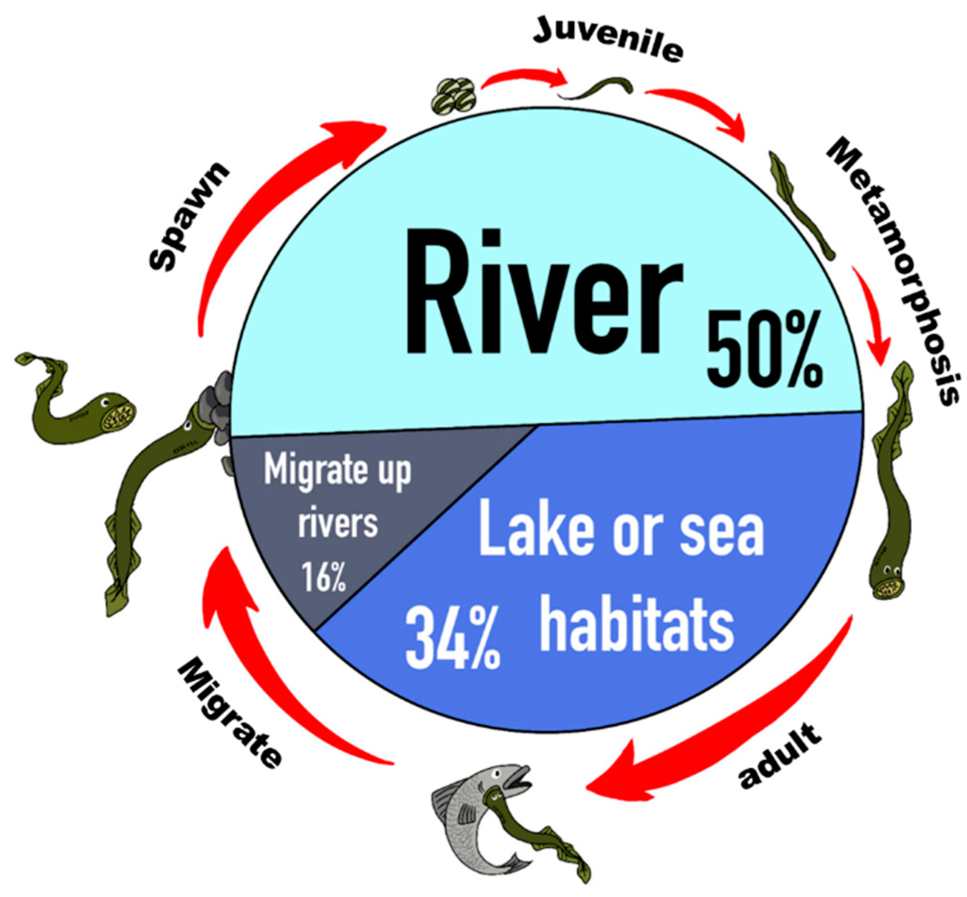
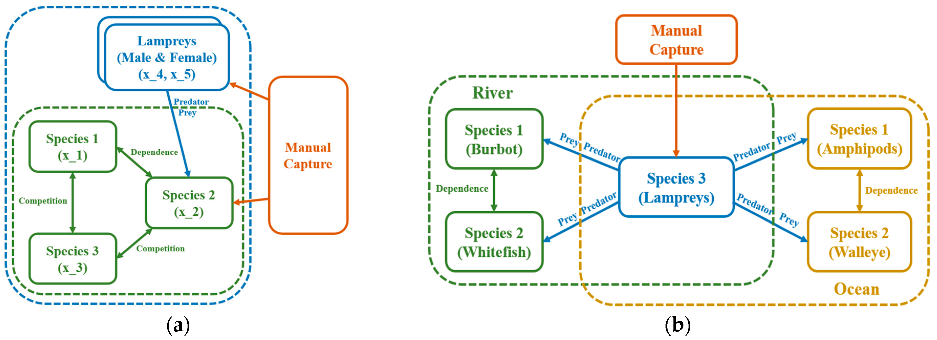
2.3. The Superiority of Using Lamprey as an Example of Instantiating the Models

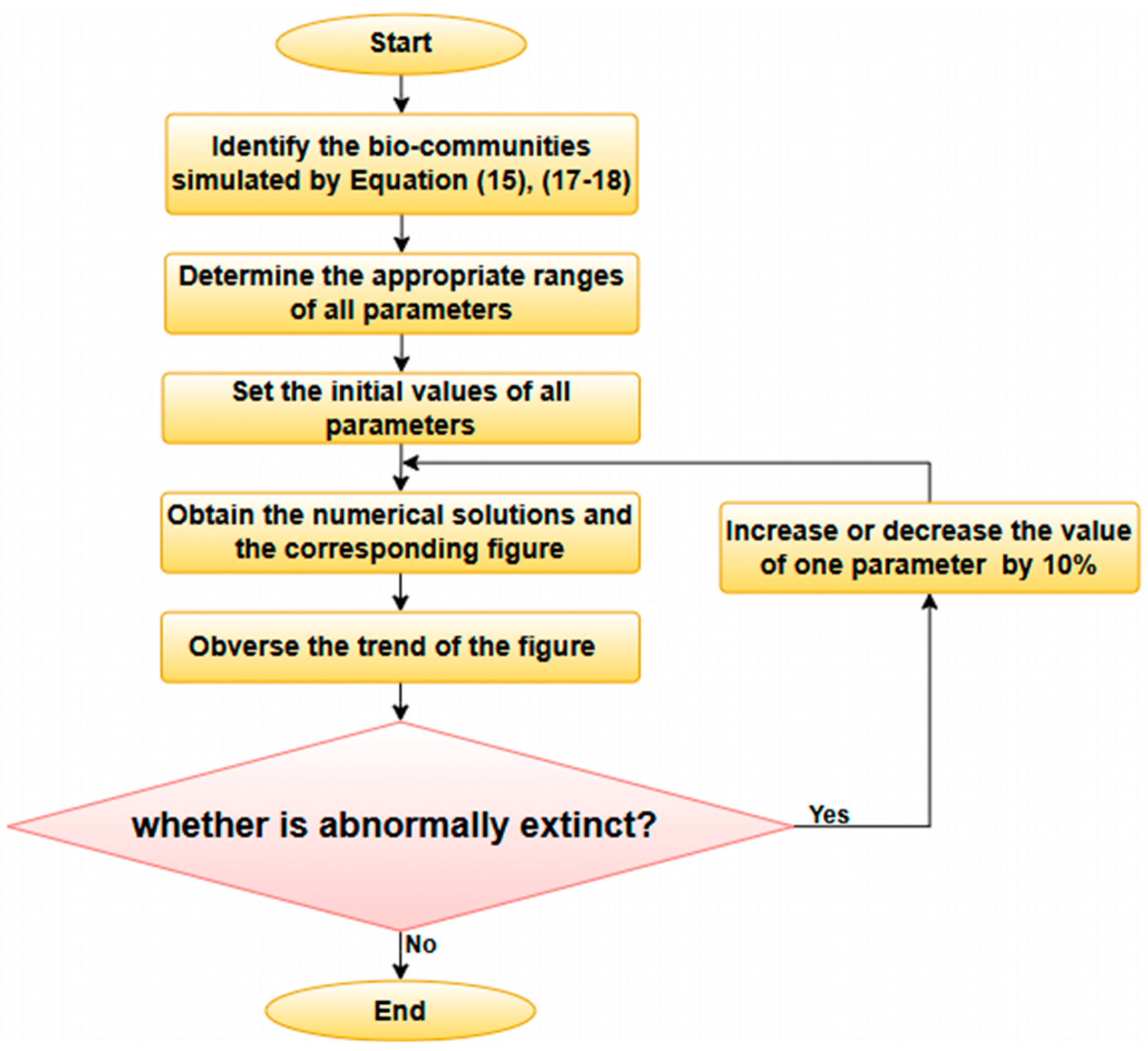
According to research, the lamprey is a kind of species with an adaptive male–female sex ratio and a kind of migratory fish that live in different environments during its lifecycle [14]. This finding is essential. This will directly affect the relevant bio-communities to varying extents. Hence, the lamprey is an ideal instantiated object for the ODE environmental models. Its lifecycle is summarized and shown in Figure 3.

It is found that there are two main environments: riverine and marine. The biggest difference between these environments is the total resources. Hence, the discussion is divided into two scenarios: riverine and marine environments. The male–female sex ratio and the environmental carrying capacity are varied while keeping other parameters constant to explore different changes in the density of species within the bio-communities.

It is worth mentioning that this optimal ODE environmental model is fundamental and universal for all of the species with the adaptive male–female sex ratio. When this optimal model is applied to different species in this category, the main parameter values that should be changed are the intensity of manual capture $e$ and environmental carrying capacity $N_i$, because although these species all belong to one category, the humanity factors and the environments situation during the corresponding lifecycle are different. Other parameters may have some differences, but they will not make much difference.

After instantiating, though the structures are different, the optimal model still remains abstract and does not instantiate other species in the bio-community where lamprey live in reality. To address this, in the riverine environment, this paper refers to the food web related to lamprey and selects Burbot and Whitefish as examples [15], applying species 1 and 2, respectively. Similarly, in the marine environment, Amphipods is set as species 1, and Walleye is set as species 2 [15]. The updated structures are shown in Figure 4.

3. Model Validation

The simulations in this paper are performed using MATLAB. Given that the simulations belong to a non-stiff problem without drastic and cliff-like changes, this paper employs MATLAB’s “ode45” solver, which applies the Runge–Kutta method, for solving the numerical solutions of the ODE model. Meanwhile, the initial conditions and values are specified for realistic starting points. MATLAB’s plotting functions are used to create the visual results to make the analysis more convenient. Due to the lack of feasible experimental conditions and officially collected data, to ensure that species in the simulated bio-community do not quickly become abnormally extinct due to unreasonable parameter values, parameter values are primary and are set based on theoretical and empirical perspectives. Hence, the detailed parameter value tunning is designed in Figure 5.

As for Figure 5, in the process of parameter value tuning, due to the different parameters in the models described by Equations (15), (17), and (18), the first step is to identify the bio-communities to be simulated. Based on the definitions of the corresponding model’s parameters and empirical rules, appropriate mathematical value ranges and initial values are then determined. Subsequently, the “ode45” solver is executed to obtain the initial numerical solutions. The most critical step is to determine whether the bio-community has undergone abnormal extinction. The quantitative criterion for this assessment is whether the density of most species drops rapidly to zero within the first 10% of the simulation time. The establishment of this criterion is primarily based on the premise that if the described condition occurs, the simulation does not reflect real-world scenarios and lacks any significance for research and analysis, rendering it incapable of yielding useful conclusions. If abnormal extinction is observed, each parameter value needs to be individually adjusted—either increased or decreased—until the abnormal extinction phenomenon disappears. Once the bio-community exhibits normal evolutionary trends, the corresponding parameter values are deemed suitable for the simulation.

Based on the above analysis, suitable values of parameters can be obtained. More details are shown as follows.

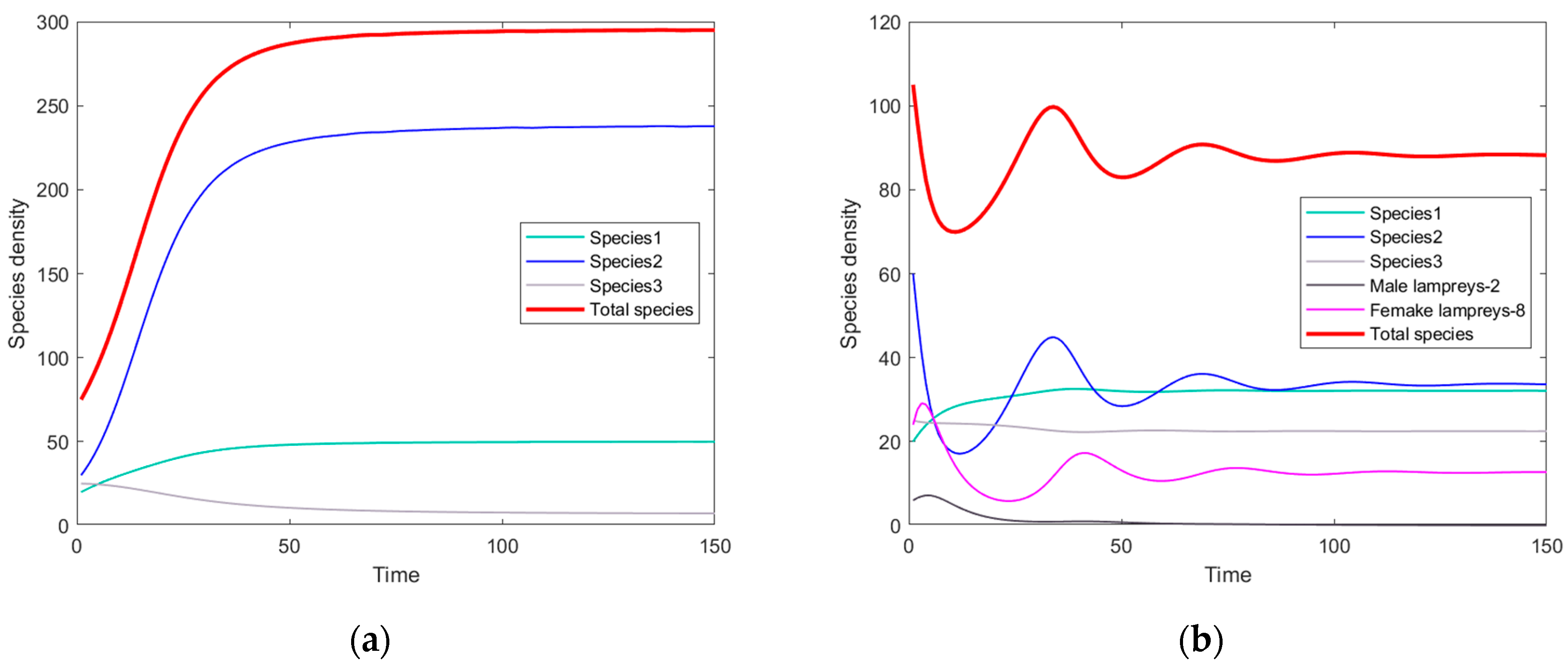
3.1. The Simulation Result of the ODE Environmental Model

Based on the above analysis, the ODE environmental model, which is before optimizing, with multiple factors, is successfully created, which is the Equation (15). Meanwhile, in order to compare the effects of different male–female sex ratios of lamprey on the bio-community affected by manual capturing factors, a control group is established, which is Equation (9). The control group established by this paper actually simulates the growth of the three species under the ideal initial state (excluding the influence of lamprey and manual capturing on species 2).

As for the simulation of the ODE environmental model before optimizing, the only change is the initial values of species densities influenced by different male–female sex ratios, while all other parameter values remain unchanged. These parameter values are submitted to Equation (15). More details are shown in

Table 3. Values of the parameters in the ODE environmental model before optimizing.

Parameter	Value	Parameter	Value
$x_1\left(t=0\right)$*	20	$x_2\left(t=0\right)$*	30
$x_3\left(t=0\right)$*	25	$x_1(t=0)$	20
$x_2(t=0)$	60	$x_3(t=0)$	25
$r_1$	0.2	$r_2$	0.1
$r_3$	0.15	$r_4$	0.2
$r_5$	0.2	$N_1$	35
$N_2$	100	$N_3$	30
$N_4$	50	$N_5$	50
$D_1$	1	$D_2$	1
$D_3$	1	$D_4$	−1
$D_5$	−1	$n_{12}$	−1
$n_{13}$	1	$n_{23}$	1
$n_{45}$	−1	e	0.015
${\sigma }_{12}$	0.2	${\sigma }_{21}$	1
${\sigma }_{13}$	0.2	${\sigma }_{23}$	0.2
${\sigma }_{31}$	0.2	${\sigma }_{32}$	0.2
${\sigma }_{45}$	1	${\sigma }_{54}$	1
${\lambda }_{24}$	0.006	${\lambda }_{42}$	0.004
${\lambda }_{25}$	0.012	${\lambda }_{52}$	0.008

* Corresponding parameters belong to the control group and are none of the other groups.

.

The simulations of Equation (15) are shown in Figure 6, Figure 7 and Figure 8. The changing trend and the total density of surviving individuals of species 1, 2, and 3 can be observed, as shown in Figure 6a. When the two influencing factors of lamprey and manual capturing are added, the male–female sex ratio of lamprey is first set at 2:8, and the reasonable parameter values of each species are brought into the Equations. The result is shown in Figure 6b.

From the results, species 2 fluctuates significantly in the early stages of development after the addition of these influencing factors, as it is most directly affected. Because of the dependence between species 1 and 2, the population growth of species 1 also slows down, and the total density of species decreases after maintenance. However, because species 3 is not directly affected by lamprey and is in a competitive relationship with species 1 and 2, although the density of species 3 decreases initially, the overall trend increases and finally stabilizes at close to 20. Therefore, species 3 indirectly benefits from the emergence of these influencing factors. At present, five species, including lamprey, gradually become stable and converge to a certain value after experiencing varying degrees of fluctuation.

At this time, the male–female sex ratio is changed to 3:7, and the result is shown in Figure 7a. The dashed line in the figure shows the development trend information of species growth when its male–female sex ratio is as before. Compared with the previous results, species 1 and 3 show almost no changes except that species 2 exhibits an initial fluctuation in the growth trend. The density of male and female lampreys increases slightly in the beginning, but the final decline trend is similar to the previous result. The male–female sex ratio of lamprey is continuously changed, and the male–female sex ratio is changed to 5:5, 7:3, and 8:2, respectively, and results are shown in Figure 7b–d.

From the above figures, it can be observed that when the male–female sex ratio is 5:5, the growth of both sexes of lamprey is maintained at a higher value. Species 2, although most directly affected by lamprey, shows an increasing trend within the range of fluctuations and ends up being more numerous than before. Further increasing the proportion of males in the lamprey population leads to a continued increase in the total density of lamprey, and the density of surviving females eventually exceeds the density of species 3.

When the final state figure, shown in Figure 7d, is obtained, the main trend information can be concluded based on the existing bio-community evolution information of other male–female sex ratios. What can be observed is that no matter how many more males start than females, they end up being fewer than females. The higher the proportion of male lamprey is, the higher the final stable density of the bio-community and lamprey is, and the final population of species 2 will increase with the increase of male lamprey. The fluctuation amplitude of male and female lampreys and species 2 decreases as the proportion of male lamprey increases, but the fluctuation duration is longer. The trend-concluded diagram is shown in Figure 8.

In general, from the above qualitative analysis of the ODE environmental model before optimization, it can be concluded that the higher the male proportion is, the more stable at a higher level the bio-community is. However, the ODE environmental model before the optimization is not suitable for the real situation due to the already-mentioned disadvantages. Therefore, more accurate quantitative analysis and the optimal ODE environmental model are necessary.

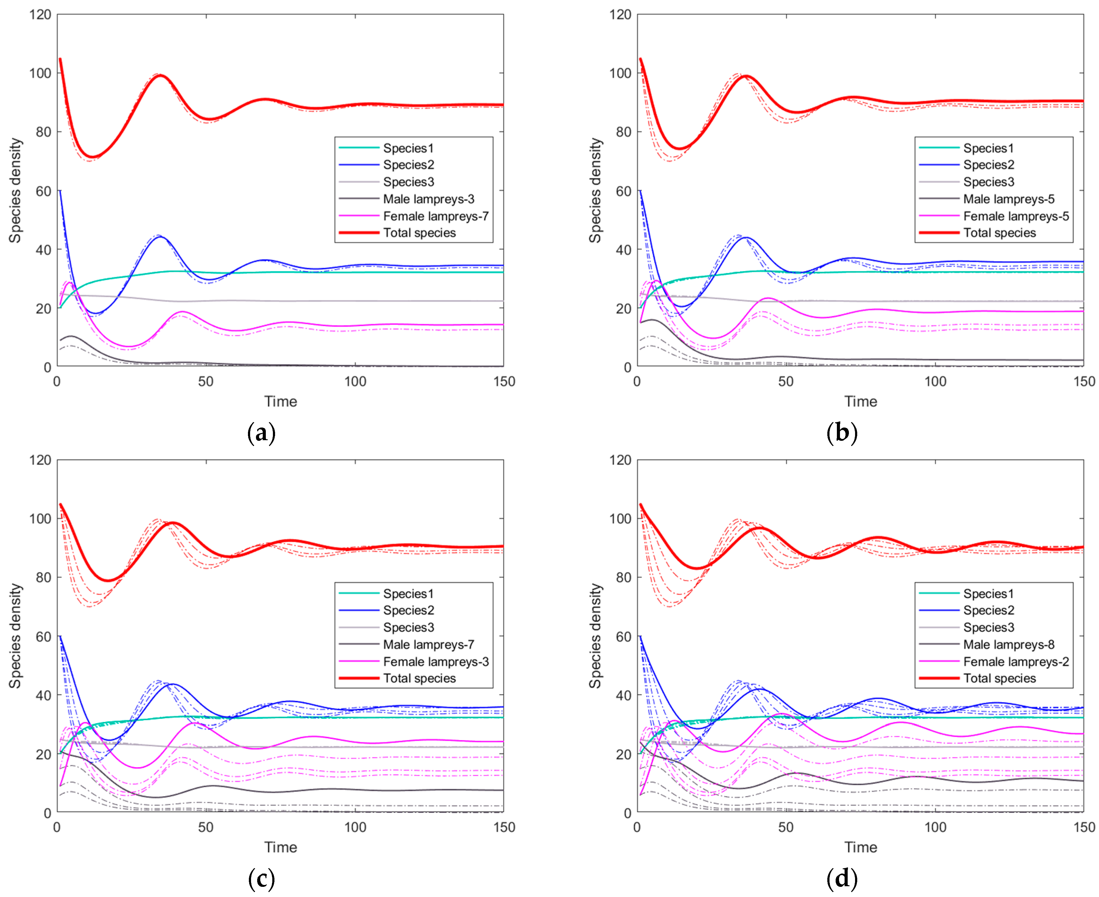
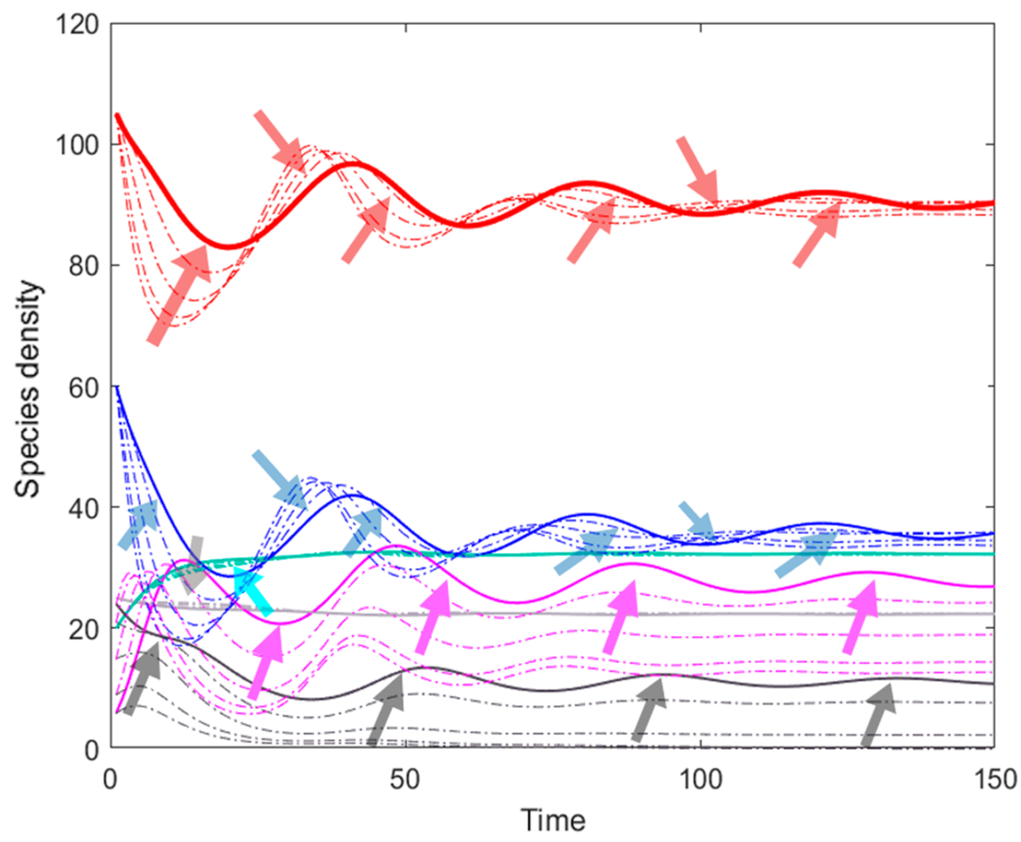
3.2. The Simulation Result of the Optimal ODE Environmental Model

According to the lifecycle, it is known that the main living environments of the lamprey are the riverine and the marine environments. The riverine environment is considered as an environment where food is scarce, while the marine environment is considered as one with plenty of food. Based on this and the drawbacks of the ODE environmental model before optimization, the optimal ODE environmental model is designed. The parameter setting process is similar to that of the ODE environmental model before optimizing. These parameter values are submitted to Equations (17) and (18). More details are shown in

Table 4. Values of the parameters in the optimal ODE environmental model.

Parameter	Value	Parameter	Value
$x_1(t=0)$	30	$x_2(t=0)$	30
$x_3(t=0)$	15	$r_1$	0.7
$r_2$	0.6	$r_3$	0.1
e	0.015	$D_1$	1
$D_2$	1	$N_1$	200
$N_2$	100	$N_1$*	1200
$N_{2 }$*	600	$n_{12}$	−1
${\sigma }_{12}$	0.2	${\sigma }_{21}$	0.2

* Corresponding parameters belong to the marine environment and are none of the others.

.

Based on the above values of the parameters, the relevant simulation results are shown as follows.

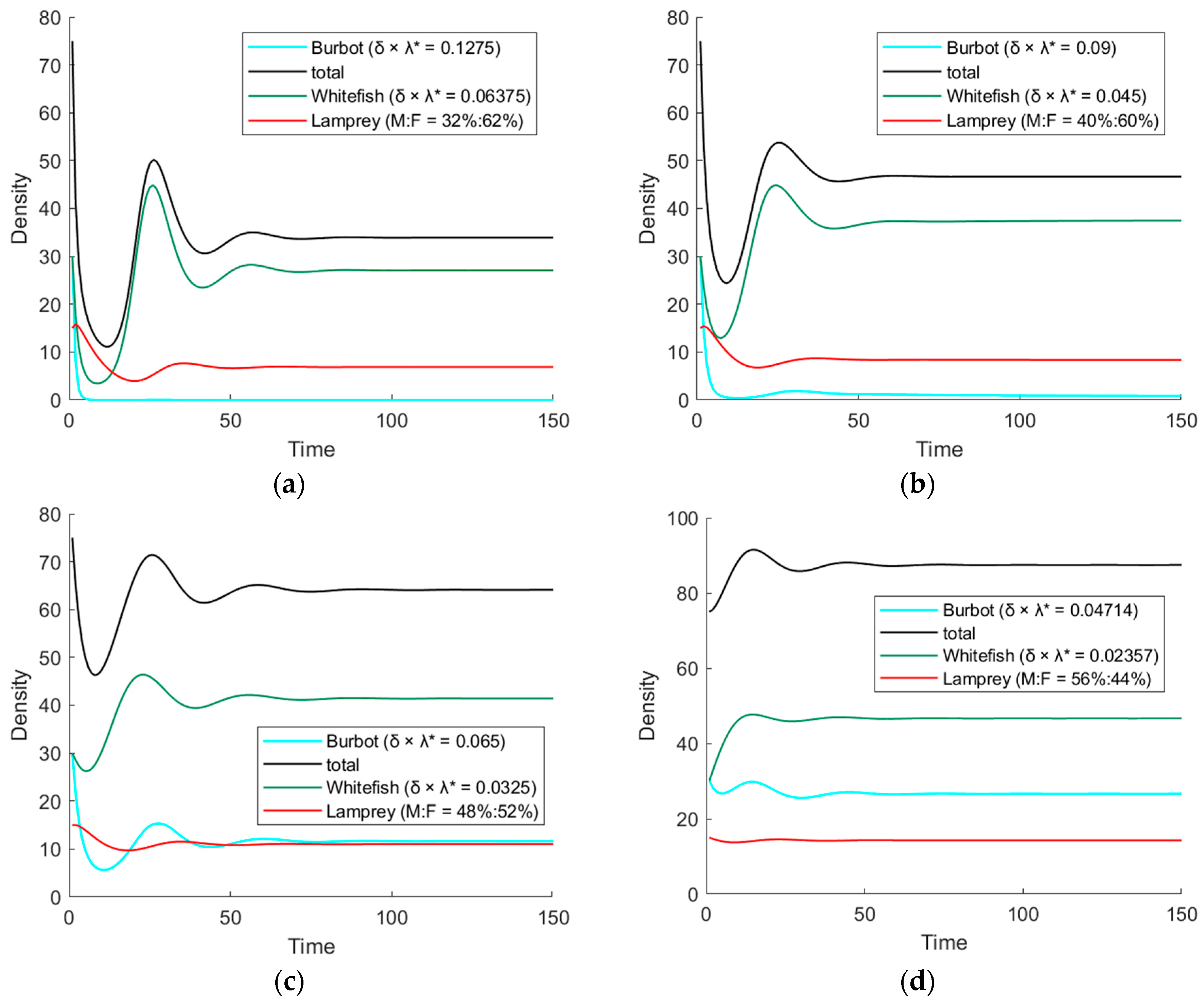
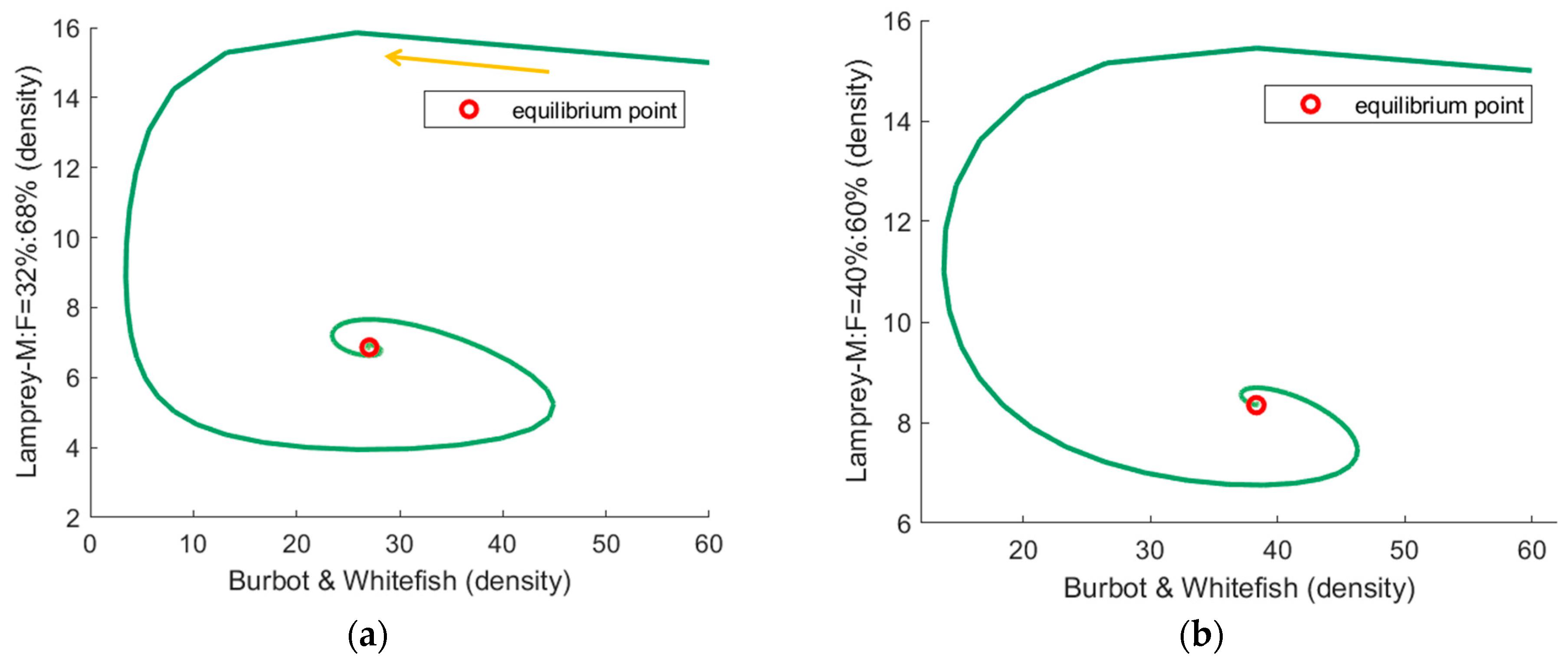
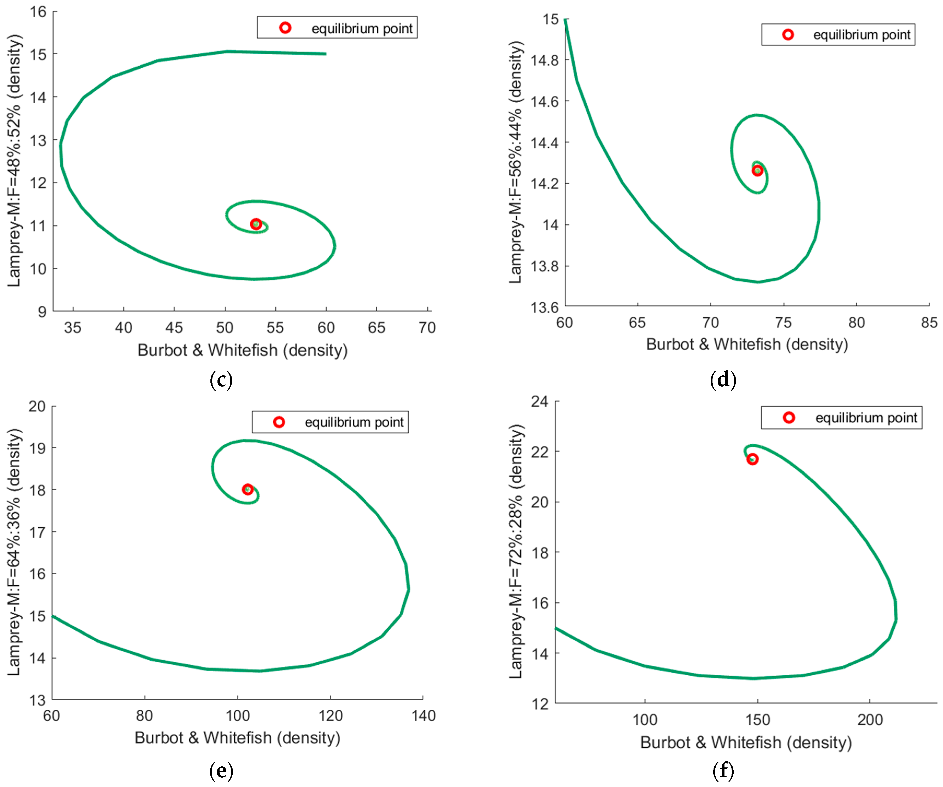
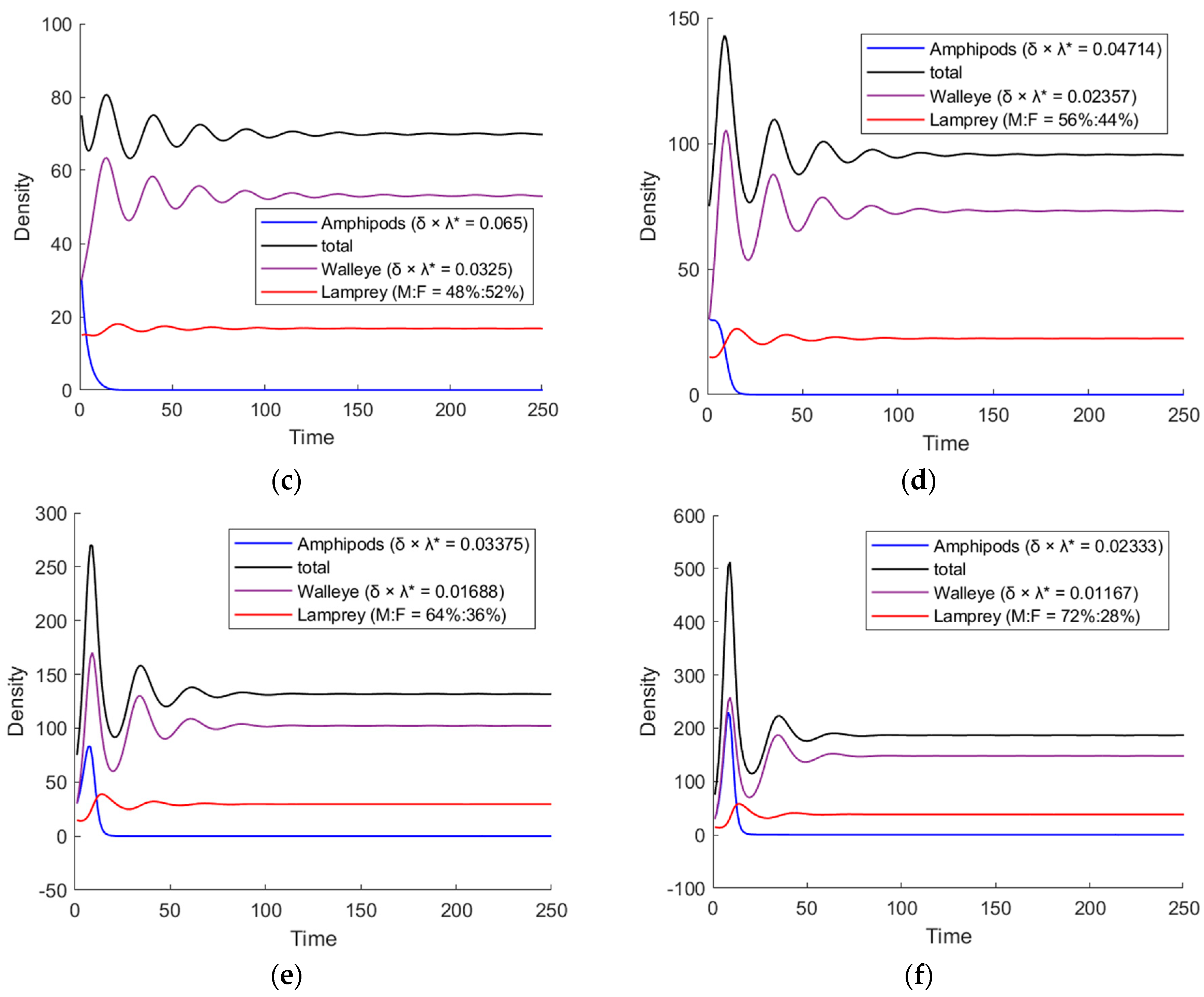
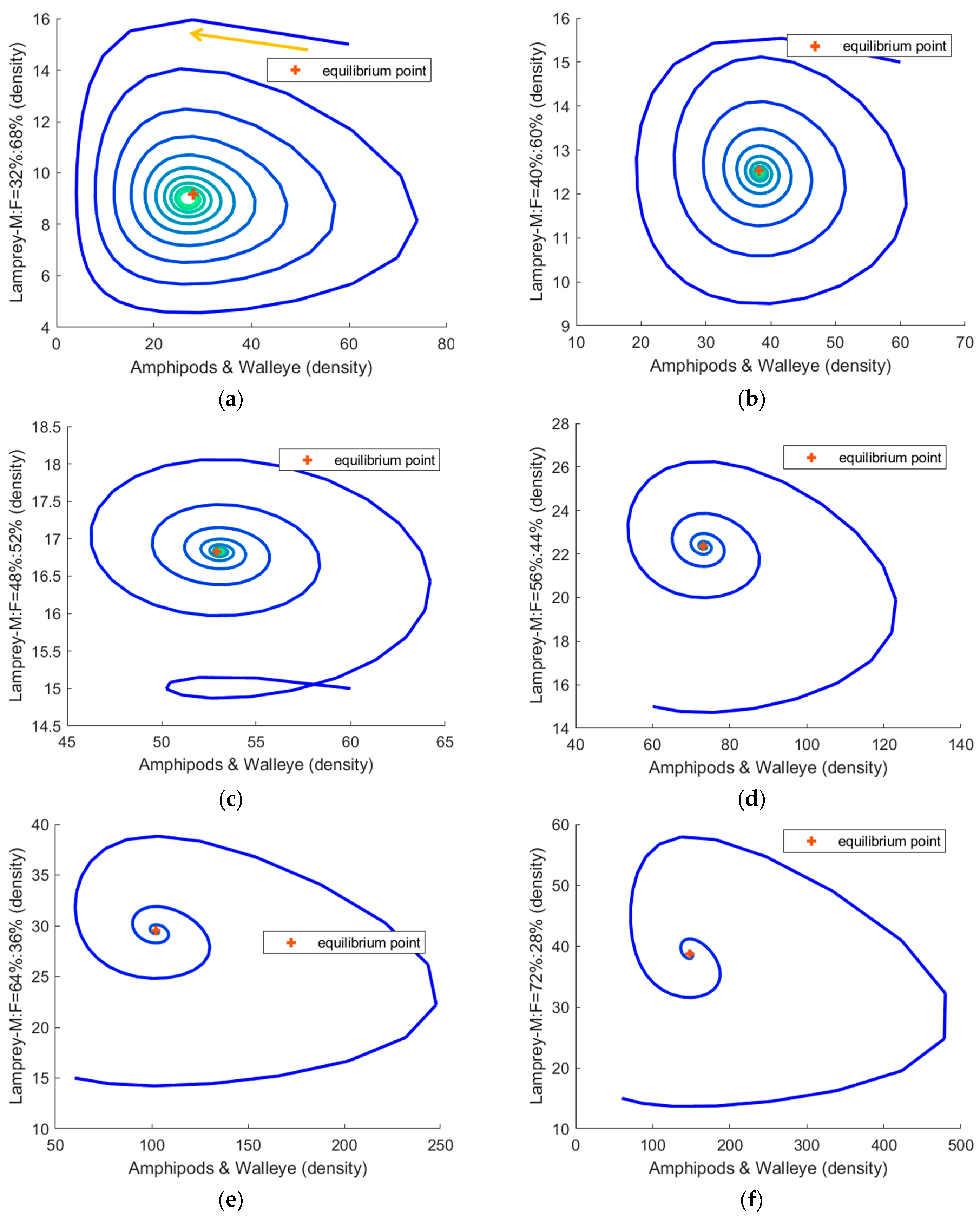
3.2.1. Stocks in Riverine Environments

In the riverine environment, Equation (17) refers to the food web related to lamprey and selects two kinds of fish: Burbot and Whitefish [15]. Species 1 and species 2 are represented by these two fish, respectively, to simulate the development of the bio-community under different male–female sex ratios of lamprey, as shown in Figure 9.

The above figures clearly visualize the growth and development status of the bio-community where lampreys with different adaptive male–female sex ratios live. It can be seen that with the increasing male proportion of lamprey, the density of Burbot and Whitefish also increases, and the total density of all species also shows a positive trend. Moreover, it is worth noting that when the male–female sex ratio of lamprey is the same as the node if the male proportion is smaller than that of the female group, the density of all species in the model will decrease initially, reach a trough (the lowest point), then rebound, and finally stabilize. However, when the male proportion of lamprey is greater than that of the female group, there is almost no significant decline in the densities in the early stage; instead, there is a rapid increase that reaches a peak and then falls back to stability.

To more clearly show the trend change speed information of state variables over time and possible long-term behaviors in this optimal model’s systems, the corresponding phase-track maps are shown in Figure 10.

From Figure 10, the faster the rate of contraction to the equilibrium point is, i.e., the fewer the number of contraction circles (as seen from the direction of the arrow in the figure), the faster the bio-community reaches a steady state. Therefore, in the figures above, the number of turns of spiral contraction to the equilibrium point in Figure 10b,f is fewer, indicating that the proportions of males and females in these two figures will reach stability faster than other male–female sex ratios. Conversely, Figure 10c,d shows a slower process of reaching stability.

Meanwhile, to quantify the fluctuation degree of the bio-community where the lamprey with the adaptive male–female sex ratio live, i.e., its stability, the relative standard deviation $R_i$ which has been mentioned in Equation (19) is further introduced to represent this index. The smaller the relative standard deviation is, the smaller the volatility is, and the more stable the bio-community of the corresponding living environment of the lifecycle is. Conversely, a larger relative standard deviation indicates greater volatility and less stability. According to the above optimal ODE environmental model and Equation (19), the relative standard deviation of the corresponding bio-community’s evolution under different male–female sex ratios is obtained. Combined with the coordinates of the equilibrium points and other information in the phase-track maps of Figure 10, the results are organized and shown in

Table 5. Summary of results for the riverine environment.

Male: Female	Steady State Fast or Slow	Equilibrium Point *	Volatility
32%:68%	Fast	(27.1, 6.9)	0.239
40%:60%	Fast	(38.3, 8,3)	0.134
48%:52%	Slow	(53.1, 11.0)	0.073
56%:44%	Slow	(73.2, 14.3)	0.025
64%:36%	Fast	(102.2, 18.0)	0.073
72%:28%	Fast	(147.9, 21.7)	0.101

* The x-coordinate is the number of Burbot and Whitefish, and the y-coordinate is the number of the lamprey.

.

The above table clearly shows the speeds of homeostasis of the bio-community, as well as coordinates of equilibrium points and relative standard deviations in a riverine environment with different male–female sex ratios of lamprey. When the male–female sex ratio is 56%:44%, the relative standard deviation of the corresponding bio-community is 0.025, which is the smallest one. This indicates that this male–female sex ratio distribution is relatively stable in the riverine environment where food is scarce, although the time for species to reach the plateau is one of the slower situations in this case.

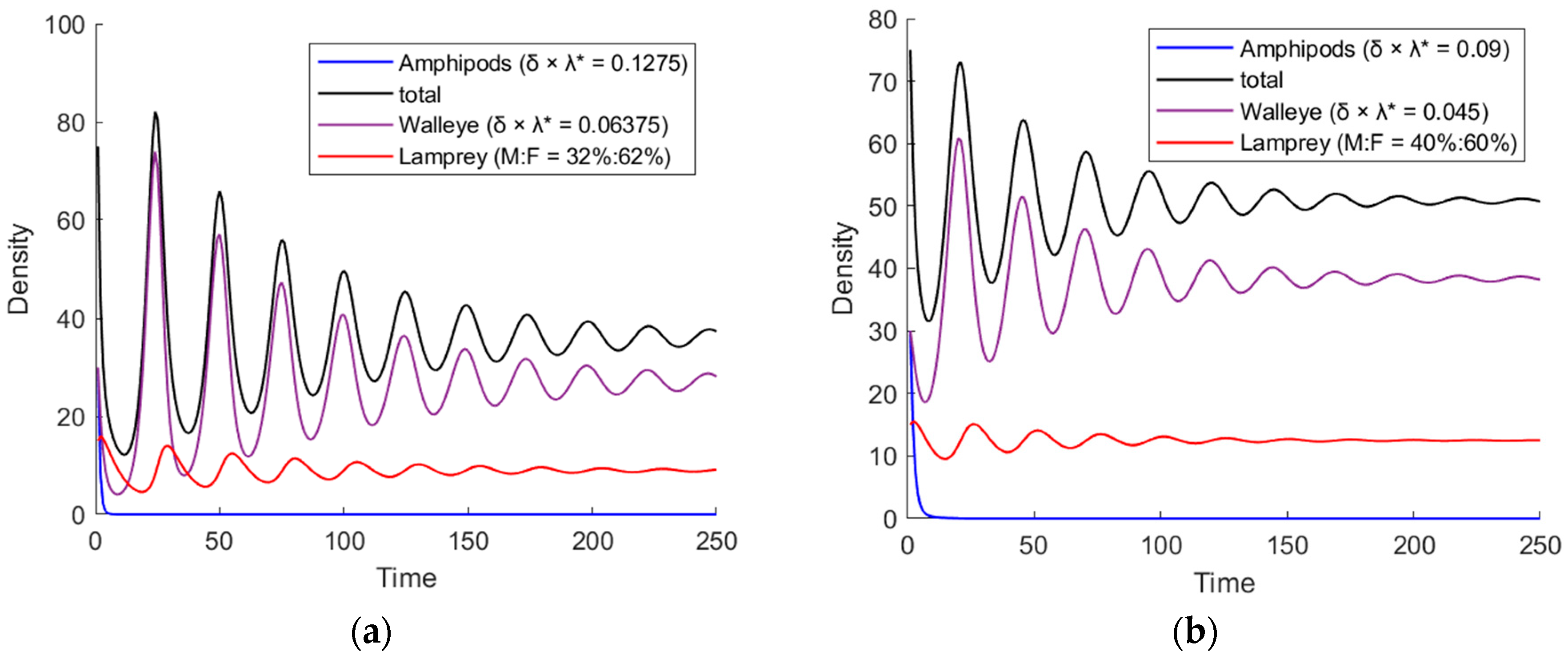
3.2.2. Stocks in Marine Environments

As lamprey swim from their riverine environment to the marine environment, the corresponding food bait and other relevant species also change. Based on the food web in the real situation, species 1 is represented by Amphipod, and species 2 is represented by Walleye [15], with the interspecific relationships remaining unchanged. The fluctuations and species densities under different male–female sex ratios after changing the environmental carrying capacity, based on Equation (18), are shown in Figure 11.

As seen from the above figures, with the increasing male proportion of lamprey, the fluctuation time of species growth quantity is shortened, and the bio-community reaches the final steady state more quickly. The total density of species in the bio-community to which lamprey belongs also increases with the increasing male proportion of lamprey. When the proportion of males is smaller than that of females, the fluctuation range of species number decreases with the increase of male proportion. However, when the male proportion exceeds the female proportion, the number of prey fluctuates more with the increasing male proportion, but the time to reach the plateau period is shortened.

To more clearly compare and display the fluctuation information in Figure 11, phase-track maps are drawn for further analysis based on the established optimal ODE environmental model of lamprey in the marine environment, as shown in Figure 12.

In the marine environment, the phase-track maps of species changes are more clear and orderly. It can be clearly observed that with the increase in the proportion of male lampreys in the bio-community, the number of contraction cycles in the phase-track maps continuously decreases in Figure 12a–f. This indicates that the rate at which the bio-community reaches a final stable state increases continuously. As in the riverine environment, the relative standard deviation, which is calculated by Equation (19), is used to quantify bio-community stability in the marine environment, as shown in

Table 6. Summary of results for the marine environment.

Male: Female	Steady State Fast or Slow	Equilibrium Point *	Volatility
32%:68%	slowest	(28.1, 9.2)	0.319
40%:60%	slower	(38.2, 12.5)	0.122
48%:52%	general	(52.9, 16.8)	0.034
56%:44%	general	(73.1, 22.3)	0.087
64%:36%	quicker	(102.2, 29.5)	0.158
72%:28%	fastest	(147.9, 38.8)	0.237

* The x-coordinate is the number of Amphipods and Walleye, and the y-coordinate is the number of lampreys.

.

As can be seen from the above table, in the marine environment with relatively abundant food, when the male–female sex ratio of lamprey is 48%:52%, the relative standard deviation is 0.034, which is the smallest among these six male–female sex ratio combinations. This indicates that the bio-community with this corresponding male–female sex ratio is in the most stable state. In this case, the steady-state duration is generalized. In the marine environment’s model experiment, the bio-community reaches the steady state slowest at the lowest male ratio, while the higher the male ratio is, the faster the bio-community reaches the steady state.

In summary, based on the optimal ODE environmental model, the bio-community is the most stable in the riverine environment when the male–female sex ratio of lamprey is 56%: 44%, with a relative standard deviation of 0.025 and a slow speed of reaching equilibrium. In the marine environment, the bio-community is most stable when the male–female sex ratio of lamprey is 48%:52%, with a relative standard deviation of 0.034 and a general speed of reaching equilibrium.

4. Discussion

From the simulation results of the optimal ODE environment model, the bio-community is most stable in the riverine environment with a male–female sex ratio of 56%:44%. The relative standard deviation is 0.025, and the speed of reaching equilibrium is slower than with other male–female sex ratios. This may be due to the relatively closed, resource-scarce environment, leading to a more stable bio-community and less variation in competition and predation relationships between biological populations. Consequently, there is normally less fluctuation in the bio-community across different adaptive male–female sex ratios, but a larger cost to maintain a stable state with a normally slower speed due to the scarce resources.

In contrast, in the marine environment, the male–female sex ratio of 48%:52% has a relative standard deviation of 0.034 and a general rate of equilibrium compared to other male–female sex ratios. The resource-rich environment, which may be more open, is more influenced by various external factors, including manual interventions, leading to possible chain effects on the bio-community. This results in relatively large fluctuations in the bio-community across different male–female sex ratios but a lower cost to maintain a stable state with a generally moderate speed due to the abundant resources.

Therefore, from the simulation results, it can be seen that different adaptive male–female sex ratios have varying effects in the different living environments of the lifecycle.

5. Conclusions and Outlooks

The primary focus of this paper is to study the effects of the species with adaptive male–female sex ratios on the bio-community. Based on the conception of the ODE environment model before optimizing, this paper constructs the optimal ODE environment model to analyze these effects. There are several innovative factors considered, including the manual capturing and lifecycle. To be more convenient to analyze and understand, based on the results of the serious research, the lamprey is set as an example of the species with the adaptive male–female sex ratio to instantiate these models. Finally, a quantitative analysis of stability is conducted using relative standard deviation and phase-track maps to examine these effects in different living environments throughout the lifecycle.

According to the results of these effects, there are directive opinions and contributions that can be concluded to help manage and protect the ecosystems and relevant bio-communities where the species with the adaptive male–female sex ratio is found. For example, by creating resource-scarce areas within resource-rich regions and restricting the multiplication of this species in these areas, the effects of management can be achieved by reducing the negative effects on the entire bio-community on the basis of ensuring that the original bio-community is not changed significantly.

As for the entire research process of this paper, although there are several innovative points considered in this paper, these are some explicit factors, and the models still cannot describe as realistic an environment as possible without considering some other implicit and more detailed factors. Meanwhile, because of the lack of official, accurate data and experimental conditions, although the setting of parameter values is reasonable and makes the bio-communities normally evolve, it lacks certain data support. This can also result in simulations that do not fully match reality. These limitations highlight areas for improvement in this paper.

For more in-depth research in the future, if the relevant departments can provide specific and professional sample data on species with the adaptive male–female sex ratio and their relevant bio-communities, it would greatly aid in studying the effects of this kind of species and the relevant bio-community. Of course, from a mathematical point of view, the construction of the entire model also deserves deeper optimization, such as the consideration of the fear factor in interspecies predation [16,17,18], the intermediate moving process in environmental change [19], the consideration of the factors of climate such as environmental temperature [20,21,22], and even the consideration of the ecological damage caused by biological invasion, which affects various aspects of the data [23]. Additionally, the ODE model set up in this paper can be extended and optimized to handle more complex dynamic cases [24,25]. A dynamic simulation would allow more factors to interfere and change in real-time, making the entire mechanism analysis more complete and closer to reality [26]. The reference coefficient for the stability of the entire bio-community can also be optimized, and multiple coefficients can be combined to characterize the real-time stability of the whole bio-community. This would facilitate the observation of the changes in the stability of the ecological environment caused by the introduction of variables such as control measures or species invasion [27].

References

1. Yan, H.; Liang, L.; Chang, Y.; Sun, B.; Su, B. Effects of inheritance and temperature on sex determination and differentiation related genes and sex ratio in fish: A review. J. Dalian Ocean. Univ. 2017, 32, 111–118. [Google Scholar] [CrossRef]
2. Yang, B.; Shao, L.; Dai, X.; Liu, Y.-H. Analysis of the Aquaculture Prospects of the Northeast Lamprey. Agro-Tech. Serv. 2017, 34, 114. [Google Scholar] [CrossRef]
3. Lu, T.-H.; Yi, X.-R. Stability and Hopf Bifurcation of the Lotka-Volterra Competition Model with Time Delay and Refuge. J. Jilin Norm. Univ. Nat. Sci. Ed. 2024, 45, 50–59. [Google Scholar] [CrossRef]
4. Xu, J.; Lou, X.; Tu, Y.; Wan, S.; Mao, R. Intra-specific and Inter-Specific Competition of Arbuscular Mycorrhizal and Ectomycorrhizal Tree Saplings in a Subtropical Phyllostachys edulis Forest. J. Jiangxi Agric. Univ. 2021, 43, 1107–1115. [Google Scholar] [CrossRef]
5. Zhang, Q.; Yeerjiang, B.; Wang, J. Gender Differences in Responses to Interspecific Competition among Dioecious Individuals of Rhamnus schneideri var. manshurica. For. Sci. 2023, 59, 33–41. [Google Scholar] [CrossRef]
6. Lv, L.; Li, X. Stability and Bifurcation Analysis in a Discrete Predator–Prey System of Leslie Type with Radio-Dependent Simplified Holling Type IV Functional Response. Mathematics 2024, 12, 1803. [Google Scholar] [CrossRef]
7. Zhang, S. Dynamical Stability Analysis of Population with Stage Structure. Master’s Thesis, Anqing Normal University, Anqing, China, 2024. [Google Scholar]
8. Liu, M.; Liu, J.; Wang, Y.; Yu, X.; Fang, X.; You, L. Improvement of the Stability of Excimer Laser Output Pulse Energy by Beam Combination. Infrared Laser Eng. 2024, 53, 135–143. [Google Scholar] [CrossRef]
9. Dang, G. Ecological Consequences of St. Lawrence Seaway Exploitation and the U.S. Response (1954–2008). Master’s Thesis, Shandong Normal University, Jinan, China, 2023. [Google Scholar]
10. Zhu, Y.G.; Li, J.; Pang, Y.; Li, Q.W. Lamprey: An important animal model of evolution and disease research. Hereditas 2020, 42, 847–857. [Google Scholar] [CrossRef] [PubMed]
11. Zou, P. Example Analysis of Mathematical Modeling in Differential Equations. Sci. Technol. Wind 2024, (05), 43–45. [Google Scholar] [CrossRef]
12. Zheng, Y.; Chang, C. Research on associative relationship of concepts based on the Lotka-Volterra Predator-Prey Model. Chin. Med. Libr. Inf. Sci. 2022, 31, 7–13. [Google Scholar]
13. Qu, Q.; Wu, W. Stability Characteristics of Multi-Model Precipitation Forecast. Meteorological 2024, 50, 420–433. [Google Scholar] [CrossRef]
14. Docker, M.F. Section 1.3.2. In Lampreys: Biology; Conservation and Control; Fish & Fisheries Series 37; Docker, M.F., Ed.; Springer: Dordrecht, The Netherlands, 2015; Volume 1, pp. 22–24. [Google Scholar]
15. Bear, R. Principles of Biology; OpenStax CNX: Houston, TX, USA, 2022; p. 75. [Google Scholar]
16. Vinoth, S.; Vadivel, R.; Hu, N.-T.; Chen, C.-S.; Gunasekaran, N. Bifurcation Analysis in a Harvested Modified Leslie–Gower Model Incorporated with the Fear Factor and Prey Refuge. Mathematics 2023, 11, 3118. [Google Scholar] [CrossRef]
17. Jia, X. Dynamics Analysis of Leslie-Gower Predator-Prey Diffusion Model with Fear Factor. Master’s Thesis, Northwest Normal University, Lanzhou, China, 2024. [Google Scholar]
18. Liu, C.; Chen, Y.; Yu, Y.; Wang, Z. Bifurcation and Stability Analysis of a New Fractional-Order Prey–Predator Model with Fear Effects in Toxic Injections. Mathematics 2023, 11, 4367. [Google Scholar] [CrossRef]
19. Yang, M. Propagation Dynamics of a Three-Species Predator-Prey Model in a Shifting Environment. Master’s Thesis, Lanzhou University, Lanzhou, China, 2023. [Google Scholar]
20. Barman, D.; Upadhyay, R.K. Modelling Predator–Prey Interactions: A Trade-Off between Seasonality and Wind Speed. Mathematics 2023, 11, 4863. [Google Scholar] [CrossRef]
21. Lv, X.; Zhang, Y.; Gao, D.; Sun, C.; Li, H. Seasonal Succession of Rotifer Communities in Northern Lake Erhai, Southwest China. J. Lake Sci. 2023, 35, 289–297. [Google Scholar]
22. Lv, C. A Predator-Prey Model with Free Boundary in a Climate Change Environment. Master’s Thesis, Southeast University, Nanjing, China, 2022. [Google Scholar]
23. Deng, S.; Guo, W.; Wen, W.; Wang, M.G.; Huang, L.P.; Chen, Z.D.; Chen, G.J.; Zhao, S.Y. The Effects of Water Eutrophication and Species Invasion on the Food Web of Xingyun Lake. Chin. Environ. Sci. 2024, 44, 932–943. [Google Scholar]
24. Wang, Z. Research on ODE Modeling Method and Application of UHVDC Converter Station. Master’s Thesis, Southeast University, Nanjing, China, 2022. [Google Scholar] [CrossRef]
25. Zhao, Q.; Niu, X. Dynamics of a Stochastic Predator–Prey Model with Smith Growth Rate and Cooperative Defense. Mathematics 2024, 12, 1796. [Google Scholar] [CrossRef]
26. Bi, Z. Spatial Pattern Behavior Analysis of Marine Organism Population Density. Master’s Thesis, Shandong University, Jinan, China, 2024. [Google Scholar] [CrossRef]
27. Liao, X. Stability Analysis of a Volterra Biological Mathematical Model Based on Constant Coefficient. J. Ningxia Norm. Univ. 2022, 43, 30–37. [Google Scholar] [CrossRef]
Figure 1. A Schematic diagram of species structure.
Mathematics 12 02298 g001
Figure 2. The structure of the optimal environmental model.
Mathematics 12 02298 g002
Figure 3. Complete life cycle of the lamprey.
Mathematics 12 02298 g003
Figure 4. (a) The instantiated ODE environmental model. (b) The instantiated optimal ODE environmental model.
Mathematics 12 02298 g004
Figure 5. The flow chart of the parameter value tunning.
Mathematics 12 02298 g005
Figure 6. (a) The bio-community evolution of three species without lampreys and manual factors in the control group. (b) The bio-community evolution with the lamprey’s male: female = 2:8 based on the ODE environmental model before optimizing.
Mathematics 12 02298 g006
Figure 7. (a) The bio-community evolution with the lamprey’s male: female = 3:7 based on the ODE environmental model before optimizing. (b) The bio-community evolution with the lamprey’s male: female = 5:5 based on the ODE environmental model before optimizing. (c) The bio-community evolution with the lamprey’s male: female = 7:3 based on the ODE environmental model before optimizing. (d) The bio-community evolution with the lamprey’s male: female = 8:2 based on the ODE environmental model before optimizing.
Mathematics 12 02298 g007
Figure 8. Trends in species evolution with the increased male-radio (The arrows represent the direction of convergence.).
Mathematics 12 02298 g008
Figure 9. (a) The riverine bio-community evolution with the lamprey’s male: female = 0.32:0.68 based on the optimal ODE environmental model. (b) The riverine bio-community evolution with the lamprey’s male: female = 0.40:0.60 based on the optimal ODE environmental model. (c) The riverine bio-community evolution with the lamprey’s male: female = 0.48:0.52 based on the optimal ODE environmental model. (d) The riverine bio-community evolution with the lamprey’s male: female = 0.56:0.44 based on the optimal ODE environmental model. (e) The riverine bio-community evolution with the lamprey’s male: female = 0.64:0.36 based on the optimal ODE environmental model. (f) The riverine bio-community evolution with the lamprey’s male: female = 0.72:0.28 based on the optimal ODE environmental model.
Mathematics 12 02298 g009aMathematics 12 02298 g009b
Figure 10. (a) The riverine bio-community evolution with the lamprey’s male: female = 0.32:0.68. (b) The riverine bio-community evolution with the lamprey’s male: female = 0.40:0.60. (c) The riverine bio-community evolution with the lamprey’s male: female = 0.48:0.52. (d) The riverine bio-community evolution with the lamprey’s male: female = 0.56:0.44. (e) The riverine bio-community evolution with the lamprey’s male: female = 0.64:0.36. (f) The riverine bio-community evolution with the lamprey’s male: female = 0.72:0.28.
Mathematics 12 02298 g010aMathematics 12 02298 g010b
Figure 11. (a) The marine bio-community evolution with the lamprey’s male: female = 0.32:0.68 based on the optimal ODE environmental model. (b) The marine bio-community evolution with the lamprey’s male: female = 0.40:0.60 based on the optimal ODE environmental model. (c) The marine bio-community evolution with the lamprey’s male: female = 0.48:0.52 based on the optimal ODE environmental model. (d) The marine bio-community evolution with the lamprey’s male: female = 0.56:0.44 based on the optimal ODE environmental model. (e) The marine bio-community evolution with the lamprey’s male: female = 0.64:0.36 based on the optimal ODE environmental model. (f) The marine bio-community evolution with the lamprey’s male: female = 0.72:0.28 based on the optimal ODE environmental model.
Mathematics 12 02298 g011aMathematics 12 02298 g011b
Figure 12. (a) The marine bio-community evolution with the lamprey’s male: female = 0.32:0.68. (b) The marine bio-community evolution with the lamprey’s male: female = 0.40:0.60. (c) The marine bio-community evolution with the lamprey’s male: female = 0.48:0.52. (d) The marine bio-community evolution with the lamprey’s male: female = 0.56:0.44. (e) The marine bio-community evolution with the lamprey’s male: female = 0.64:0.36. (f) The marine bio-community evolution with the lamprey’s male: female = 0.72:0.28.
Mathematics 12 02298 g012