Symbolic Computation of the Lie Algebra se(3) of the Euclidean Group SE(3): An Application to the Infinitesimal Kinematics of Robot Manipulators

Abstract

This paper reports an application of the Lie algebra $se\left(3\right)$ of the Euclidean group $SE\left(3\right)$, which is isomorphic to the theory of screws in the velocity and acceleration analyses of serial manipulators. The symbolic computation of the infinitesimal kinematics allows one to obtain algebraic expressions related to the kinematic characteristics of the end effector of the serial manipulator, while in the case of complex manipulators, numerical computations are preferred owing to the emergence of long terms. The algorithm presented enables the symbolic computation of the velocity and acceleration characteristics of the end effector in serial manipulators in order to allow the compact and efficient modeling of velocity and acceleration analyses of both parallel and serial robotic manipulators. Unlike other algebras, these procedures can be extended without significant effort to higher-order analyses such as the jerk and jounce.

1. Introduction

Over the past few decades, interest in both academia and industry for developing robotic manipulators has increased considerably due to their potential applications. The repetitive and precise applications of robotic manipulators have been complemented by activities in which robots must perform unplanned tasks, but which need to be executed in real time. Thus, nowadays robotic manipulators require highly reliable mathematical resources for their performance.

The study of rigid bodies in motion is one of the most influential topics in modern robotics; e.g., industrial robot arms are a classical reference. A group can be defined as the abstraction of the properties of symmetry operations. In kinematics, the group of rigid transformations is called the Special Euclidean group $SE\left(3\right)$, which is investigated in depth by means of the Lie algebra $se\left(3\right)$. Perhaps the most comprehensive contributions to the rigid body motion related to the Lie algebra $se\left(3\right)$ can be found in the theory of screws developed by Ball [1] at the beginning of the century. After the pioneering work of Ball, it took several decades for the screw theory to be revalorized thanks to the contributions of Hunt [2] and Phillips [3]. Afterward, the isomorphism between the screw theory and the Lie algebra $se\left(3\right)$ of the Special Euclidean group $SE\left(3\right)$ led to remarkable productivity within modern differential geometry and Lie group theory; see, for instance, [4,5]. Wu and Carricato [6] reported a method to identify Lie triple screw systems of the Lie algebra $se\left(3\right)$ based on algebraic Lie group theory and descriptive screw theory and their relationship with the exponential motion manifolds of the Lie triple screw systems in dual quaternion representation. It is known that a curve in $SE\left(3\right)$ whose tangent vector the left or right invariant representation is a curve in $se\left(3\right)$ can be used to describe the general continuous motion of a rigid body. Zhang et al. [7] developed a matrix method based on the geometric properties of a pair of conjugate axodes equivalent to a curve in $se\left(3\right)$ in algebras to achieve this result. Sanchez-Garcia et al. [8] investigated the mobility of parallel manipulators by means of screw theory in which the intersection of subalgebras of Lie algebra, $se\left(3\right)$, of the special Euclidean group, $SE\left(3\right)$, associated with the limbs of the parallel manipulator plays a central role. Chen et al. [9] introduced a multisymplectic Lie algebra variational integrator for simulating the dynamics of flexible multibody systems.

Mathematically, a Euclidean group is the characteristic group of isometries of a Euclidean space ${\mathbb{E}}^n$ where n denotes the dimension of the space and its transformations preserve the Euclidean distance between any pair of points of the physical space. The configuration of the group depends on the dimension n of the space and is commonly notated as $E\left(n\right)$. Note that the Euclidean group $E\left(n\right)$ consists of all translations, rotations, and reflections of ${\mathbb{E}}^n$, as well as arbitrary finite combinations of these transformations. The Euclidean group can be considered the symmetry group of the space itself and contains the group of symmetries of any subset of that space. A Euclidean isometry may be direct or indirect, depending on whether it preserves the parity of the subsets. In that regard, direct Euclidean isometries can be grouped into the special Euclidean group $SE\left(n\right)$, a subgroup of $E\left(n\right)$ whose elements are called rigid motions or Euclidean motions. It is worth emphasizing that they comprise arbitrary combinations of translations and rotations, but reflections are excluded. The special group $SE\left(n\right)$ is among the oldest, at least in the cases of dimensions 2 and 3, being implicitly studied long before the concept of the group was envisioned. The contribution is focused on the special Euclidean group $SE\left(3\right)$. Euclidean groups in addition to being topological groups are also catalogued as Lie groups, after Marius Sophus Lie, and therefore, the concepts of infinitesimal calculus can be immediately adapted to this configuration.

Screw theory is perhaps just another algebra for the kinematic analysis of robotic manipulators; however, its effectiveness is well proven in geometric interpretation. For example, the quaternion algebra works very well in velocity analysis, but its extension to acceleration analysis encounters difficulties that its followers have not solved satisfactorily, so it is often necessary to resort to devices that escape mathematical rigor, as is the case with exponential methods. Screw theory, as a number of investigations have shown, has largely outperformed higher-order analysis. Therefore, the contribution of this possible contribution will certainly meet the expectations of users of three-dimensional kinematics of robotic manipulators.

In mathematics and computer science, symbolic computation, also known as algebraic computation, is a scientific area that refers to the study and development of algorithms and software for manipulating mathematical expressions derived from diverse disciplines of knowledge and other mathematical objects in general. Symbolic computation is a highly reliable strategy in the validation of mathematical procedures that attempt to model the behavior of natural phenomena in which the use of mathematical formulas plays a preponderant role. In addition, and beyond modeling physical phenomena, in this case, the kinematics of robotic systems, algebraic computation is widely used in areas such as control engineering, in model-based strategies that require solving Coupled Nonlinear Systems of Variable-Order Fractional PDEs, especially if higher-order kinematic variables need to be controlled [10,11].

Within kinematic analysis, one of the fields where computational methods are usually employed is in position analysis, especially in parallel manipulators. Nearly forty years ago, Freudenstein referred to the challenge of solving polynomial expressions from the inverse kinematics problem of the 7R spatial linkage as the “Mount Everest of kinematics”. Since then, there has been a continuous increase in the publication of specialized papers introducing new kinematic analysis strategies or refining existing methods, leading to a significant re-evaluation of kinematics. Despite the considerable progress made, challenges persist in addressing these analyses. Research in this area can be categorized into three main approaches: (i) iterative numerical solutions, (ii) the implementation of auxiliary sensors, and (iii) polynomial solutions. Iterative methods are straightforward but face limitations such as incomplete solutions, convergence issues, and the need for good initial estimates. The second approach requires a physical prototype. Polynomial methods, on the other hand, mitigate these challenges and provide a reliable way to determine the feasible poses of a parallel manipulators for a given set of prescribed generalized coordinates.

Moreover, with the advent of symbolic software, it is possible to generate the symbolic equations of practically any engineering problem. In this paper, we present symbolic procedures generated with the software Maple ver. 2022 associated with the operations of the Lie algebra $se\left(3\right)$ of the Euclidean group $SE\left(3\right)$. These procedures are general and can be applied without major difficulties in the kinematic analysis of robotic manipulators.

The aim of the paper is not to discuss or provide new insights into the Lie algebra $se\left(3\right)$ of the Euclidean Group $SE\left(3\right)$. Rather, the focus and contribution of the paper are as follows: (a) to provide symbolic procedures that allow the compact and efficient modeling of velocity and acceleration analyses of both parallel and serial robotic manipulators; (b) to show that the Lie algebra structure allows us to easily provide computational algorithm operations and analyses compared to other algebras, such as the quaternion algebra, which lead to unintuitive methods that are not always generalizable or that are difficult to implement for complex robotic structures; and (c) to show that these results can easily be extended to higher-order kinematic analyses (third and fourth time derivatives) without significant effort.

The rest of this contribution is organized as follows: in Section 2, the fundamentals of the Lie algebra of the Euclidean group are presented and related to fundamental concepts of the kinematics of multibody systems, such as the velocity state and the reduced acceleration state of a rigid body and open kinematic chains. In Section 3, some operations of Lie Algebra implemented in Maple used in kinematic analysis are reported. Then, in Section 4, applications and numerical examples of this contribution to the kinematic analysis of representative open kinematic chains are presented. Finally, Section 5 concludes this paper.

2. Theory

2.1. Plücker Coordinates

The homogeneous coordinates of a segment line in space are known as Plücker coordinates and were introduced in the 19th century by Julius Plücker [12,13]. The Plücker coordinates are also known as Grassmann coordinates and provide a logical beginning to introduce the basics of the theory of screws.

In physics, a rigid body or object is a solid body in which deformation is zero or so small that it can be disregarded. Thus, the distance between two arbitrary points of a rigid body remains constant even though the body undergoes external forces or moments. The pose of a rigid body refers to the information required to determine the position of the center of mass of the rigid body, as well as its orientation or attitude. In the general case, the pose of a rigid body is defined by six parameters: three for the position and three for the orientation. The number of parameters considered in the pose of the rigid body is called the degrees of freedom of the rigid body. Considering that, in a line segment, the rotation around an axis along the line itself does not affect the pose of the line, then four parameters are sufficient to determine the pose of a line segment.

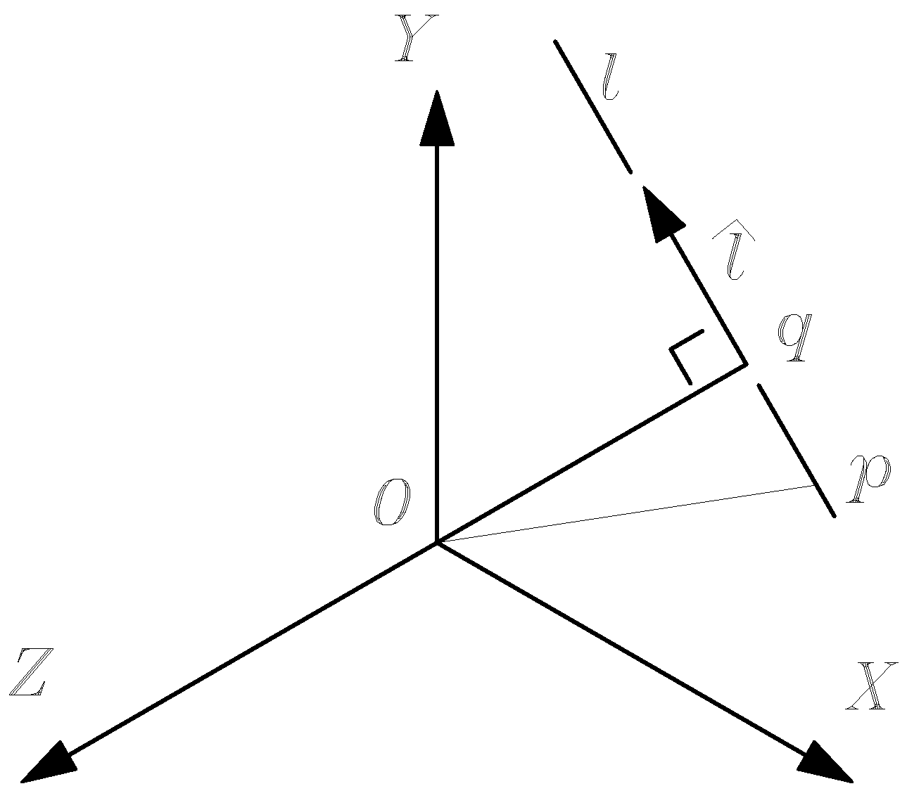
Figure 1 shows a segment line l passing through point p. According to the reference frame $O\text{\_}XYZ$, the line l can be characterized entirely by introducing the unit vector $\widehat{\mathit{l}}$ and the position vector $\mathit{p}$ of point p. Then, it is possible to define a vector $\mathit{L}\in {\mathbb{R}}^6$ formed with the concatenation of two vectors $\widehat{\mathit{l}}$ and $\mathit{m}$ as follows

$$\begin{array}{c}\hfill \mathit{L}=\left[\begin{array}{c}\widehat{\mathit{l}}\\ \mathit{m}\end{array}\right]\end{array}$$

(1)

where $\mathit{m}=\widehat{\mathit{l}}\times \mathit{q}$ is the moment vector of the unit vector $\widehat{\mathit{l}}$ about the origin O of the reference frame $O\text{\_}XYZ$. Note that vector $\mathit{q}$ is normal to vector $\widehat{\mathit{l}}$. Naturally, any point of the line l may be used to compute the moment vector $\mathit{m}$. For example, let us consider that $\mathit{q}=\mathit{p}+\lambda \widehat{\mathit{l}}$, where $\lambda \in \mathbb{R}$. Then, it follows that

$$\begin{array}{c}\hfill \mathit{m}=\mathit{q}\times \widehat{\mathit{l}}=(\mathit{p}+\lambda \widehat{\mathit{l}})\times \widehat{\mathit{l}}=\mathit{p}\times \widehat{\mathit{l}}+\lambda (\widehat{\mathit{l}}\times \widehat{\mathit{l}})=\mathit{p}\times \widehat{\mathit{l}}\end{array}$$

(2)

The parameters involved in Equation (2) are called the Plücker coordinates of the line segment. It is straightforward to demonstrate that Equation (2) has two redundancies: (i) $\widehat{\mathit{l}}$ is a unit vector, which implies that $\mid \widehat{\mathit{l}}\mid =1$; (ii) it must satisfy that $\widehat{\mathit{l}}·\mathit{m}=0$. Then, a line in Plücker coordinates can be characterized by only four parameters.

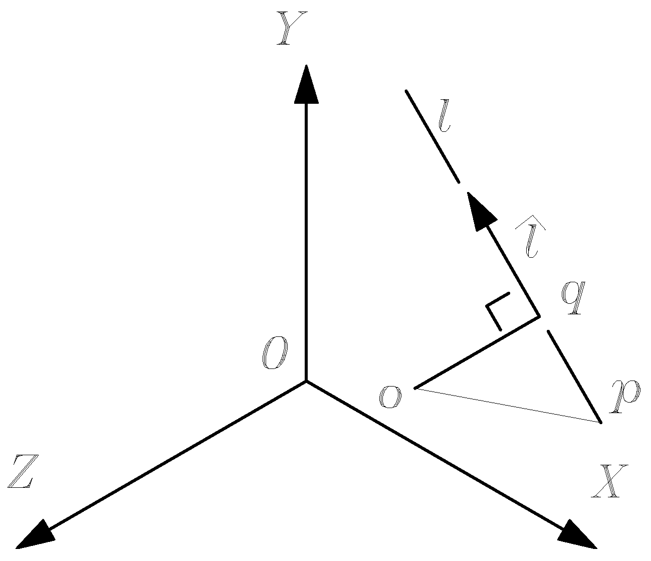
Figure 2 shows a line l passing through point p. Let us consider an arbitrary point o. The moment vector ${\mathit{m}}_o$ produced by the line l around the point o may be computed as

$$\begin{array}{c}\hfill {\mathit{m}}_o=(\mathit{p}-\mathit{o})\times \widehat{\mathit{l}}=\mathit{p}\times \widehat{\mathit{l}}-\mathit{o}\times \widehat{\mathit{l}}=\mathit{m}-\mathit{o}\times \widehat{\mathit{l}}\end{array}$$

(3)

Hence

$$\begin{array}{c}\hfill {\mathit{m}}_o=\mathit{m}-\mathit{o}\times \widehat{\mathit{l}}\end{array}$$

(4)

Furthermore, according to point q, the vector ${\mathit{m}}_o$ may be computed as

$$\begin{array}{c}\hfill {\mathit{m}}_o=(\mathit{q}-\mathit{o})\times \widehat{\mathit{l}}\end{array}$$

(5)

Premultiplying both sides of Equation (5) by $\widehat{\mathit{l}}$, it follows that

$$\begin{array}{c}\hfill \widehat{\mathit{l}}\times {\mathit{m}}_o=\widehat{\mathit{l}}\times [(\mathit{q}-\mathit{o})\times \widehat{\mathit{l}}]\end{array}$$

(6)

However, the expulsion property of the triple cross product leads to

$$\begin{array}{c}\hfill \widehat{\mathit{l}}\times [(\mathit{q}-\mathit{o})\times \widehat{\mathit{l}}]=\widehat{\mathit{l}}·\widehat{\mathit{l}}(\mathit{q}-\mathit{o})-[\widehat{\mathit{l}}·(\mathit{q}-\mathit{o})]\widehat{\mathit{l}}=\mathit{q}-\mathit{o}\end{array}$$

(7)

Hence,

$$\begin{array}{c}\hfill \mathit{q}=\mathit{o}+\widehat{\mathit{l}}\times {\mathit{m}}_o\end{array}$$

(8)

The reciprocal product between two lines is one of the highlights of Plücker coordinates. Let $l_1$ and $l_2$ be two lines whose Plücker coordinates are established as follows:

$$\begin{array}{c}\hfill {\mathit{L}}_1=\left[\begin{array}{c}{\widehat{\mathit{l}}}_1\\ {\mathit{m}}_1\end{array}\right],{\mathit{L}}_2=\left[\begin{array}{c}{\widehat{\mathit{l}}}_2\\ {\mathit{m}}_2\end{array}\right]\end{array}$$

(9)

Moreover, according to Equation (4), it follows that

$$\begin{array}{c}\hfill {\mathit{m}}_1={\mathit{m}}_2-{\mathit{p}}_1\times {\widehat{\mathit{l}}}_2\end{array}$$

(10)

The application of the inner product between the unit vector ${\widehat{\mathit{l}}}_1$ and the right side of Equation (10) yields

$$\begin{array}{c}\hfill {\widehat{\mathit{l}}}_1·({\mathit{m}}_2-{\mathit{p}}_1\times {\widehat{\mathit{l}}}_2)={\widehat{\mathit{l}}}_1·{\mathit{m}}_2+{\widehat{\mathit{l}}}_2·{\mathit{m}}_1\end{array}$$

(11)

where the term ${\widehat{\mathit{l}}}_1·({\mathit{m}}_2-{\mathit{p}}_1\times {\widehat{\mathit{l}}}_2)$ is known as the reciprocal product between two lines, and it is notated as ${\mathit{L}}_1\ast {\mathit{L}}_2$. That is to say,

$$\begin{array}{c}\hfill {\mathit{L}}_1\ast {\mathit{L}}_2={\widehat{\mathit{l}}}_1·{\mathit{m}}_2+{\widehat{\mathit{l}}}_2·{\mathit{m}}_1\end{array}$$

(12)

The geometry of lines found in the screw theory is a formidable ally for its mathematical formulation. For example, a screw, which is notated as $, can be represented in Plücker coordinates as follows:

$$\begin{array}{c}\hfill \$=\left[\begin{array}{c}\widehat{\mathit{s}}\\ {\mathit{s}}_O\end{array}\right]\end{array}$$

(13)

where the unit normalized vector $\widehat{\mathit{s}}$ is known as the primal part of the screw, and it occurs along the axis of the screw, which is called the Mozzi’s axis. Meanwhile, ${\mathit{s}}_O$ is the moment produced by $\widehat{\mathit{s}}$ around the reference pole O. The vector ${\mathit{s}}_O$ is called the dual part of the screw, and it is computed as

$$\begin{array}{c}\hfill {\mathit{s}}_O=h\widehat{\mathit{s}}+{\mathit{r}}_{Q/O}\times \widehat{\mathit{s}}\end{array}$$

(14)

where h is the pitch of the screw, while ${\mathit{r}}_{Q/O}$ is a vector beginning at the reference pole O and ending in arbitrary point Q of Mozzi’s axis. Mozzi’s axis is the Instantaneous Screw Axis (ISA). In the rotational displacement, the pitch h of the screw vanishes, and therefore, in this case, we have that

$$\begin{array}{c}\hfill \$=\left[\begin{array}{c}\widehat{\mathit{s}}\\ {\mathit{r}}_{Q/O}\times \widehat{\mathit{s}}\end{array}\right]\end{array}$$

(15)

On the other hand, in the translational displacement, the pitch h of the screw goes to infinity, and therefore, it follows that

$$\begin{array}{c}\hfill \$=\underset{h\to \infty }{\lim }\left[\begin{array}{c}\widehat{\mathit{s}}\\ h\widehat{\mathit{s}}+{\mathit{r}}_{Q/O}\times \widehat{\mathit{s}}\end{array}\right]=\left[\begin{array}{c}\underset{h\to \infty }{\lim }\widehat{\mathit{s}}\\ \\ \underset{h\to \infty }{\lim }(h\widehat{\mathit{s}}+{\mathit{r}}_{Q/O}\times \widehat{\mathit{s}})\end{array}\right]=\left[\begin{array}{c}\mathbf{0}\\ \widehat{\mathit{s}}\end{array}\right]\end{array}$$

(16)

2.2. Chasles’ Theorem

Theorem 1

(Euler’s Theorem). “By arbitrarily rotating a sphere around its center, it is always possible to find a diameter whose position is equal to the initial position in spite of the rotation.” [14]

One element of the Euclidean group that has attracted the most attention is that corresponding to rotational motion. Based on Euler’s pioneering work, it is possible to establish that any spatial displacement of a rigid body that maintains a constant or fixed point produces an axis with constant orientation. Moreover, Euler elegantly concluded that a composition of arbitrary rotations about the same point is equivalent to a single rotation about a new axis, which is designated as Euler’s pole. Motions satisfying these conditions have an algebraic structure which is designated as the special orthogonal group $SO\left(3\right)$ of the Euclidean group $SE\left(3\right)$ and whose dimension is 3. Mozzi extends Euler’s theorem, concluding that the displacement of a rigid body is equivalent to a rotation around an axis passing through the center of mass of the body followed by a translation in an arbitrary direction. As a prelude to the celebrated theorem of Chasles, Mozzi was able to glimpse that in the displacement of the rigid body, there are points of the rigid body that translate with the same intensity along axes parallel to the axis of rotation. In 1904, Whittaker was able to formally state that “A rotation about any axis is equivalent to a rotation by the same angle about any axis parallel to it, together with a simple translation in a direction parallel to the axis itself”.

Theorem 2

(Chasles’ Theorem). “The general motion of a rigid body in space can be expressed as a translational motion along a helical axis, called the Mozzi axis, preceded by a rotational motion around an axis parallel to the Mozzi axis.” [15,16]

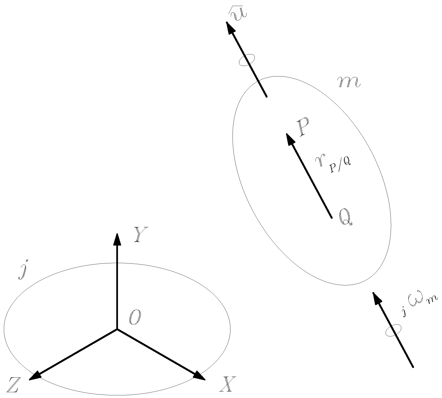
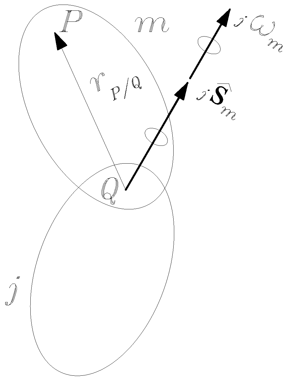
Figure 3 shows a rigid body m in general motion with respect to another body j or reference frame $O\text{\_}XYZ$. Assuming that $\widehat{\mathit{u}}$ is a unit vector along the ISA then the angular velocity vector ${}^j{\mathit{\omega }}^m$ of body m with respect to body j may be expressed as ${}^j{\mathit{\omega }}^m={}_j{\omega }_m\widehat{\mathit{u}}$. On the other hand, let us consider two points P and Q attached to the ISA, where, in general, $P\ne Q$. Then, the velocity vectors of points P and Q may be related as

$$\begin{array}{c}\hfill {\mathit{v}}_P={\mathit{v}}_Q+{}^j{\mathit{\omega }}^m\times {\mathit{r}}_{P/Q}\end{array}$$

(17)

where ${\mathit{r}}_{P/Q}$ is the position vector of point P with respect to point Q. Taking into account that ${\mathit{r}}_{P/Q}=r_{P/Q}\widehat{\mathit{u}}$, it follows that

$$\begin{array}{c}\hfill {\mathit{v}}_P={\mathit{v}}_Q+{}^j{\mathit{\omega }}^m\times {\mathit{r}}_{P/Q}={\mathit{v}}_Q+\left({}_j{\omega }_m\widehat{\mathit{u}}\right)\times \left(r_{P/Q}\widehat{\mathit{u}}\right)={\mathit{v}}_Q\end{array}$$

(18)

By mathematical induction, it is concluded that all the points on the ISA have the same velocity vector. Other interesting properties of Chasles’ theorem are the following:

• The velocity component along the Mozzi axis is the same for all points on the body m.
• The velocity component of any point of the body m along an axis perpendicular to the ISA is null.
• The velocity vector of any point of the body m lies in a plane defined by two vectors; the first one is parallel to the ISA, while the second one is normal to the ISA and to the position vector of the point of interest and an arbitrary point on the ISA.

2.3. The Lie Algebra $se\left(3\right)$ of the Euclidean Group $SE\left(3\right)$

The special Euclidean group $SE\left(3\right)$ is a Lie group composed of a set of rigid body motions and has an associated Lie algebra $se\left(3\right)$. The real space $SE\left(3\right)$ is a six-dimensional manifold where the dimension is the number of degrees of freedom of a rigid body freely moving in space. In physics, Lie groups emerge as symmetry groups of physical systems, and their Lie algebras may be considered as infinitesimal symmetry motions. In this section, the operations and properties of the Lie algebra $se\left(3\right)$ of the Euclidean group $SE\left(3\right)$ are briefly explained from the point of view of the kinematic state of a rigid body. To enumerate the operations of the Lie $se\left(3\right)$ of the Euclidean group $SE\left(3\right)$ it must be considered that it is isomorphic to the theory of screws [1] and the motor algebra [17].

Let us consider that a rigid body m is in general motion with respect to another body j or reference frame $O\text{\_}XYZ$. Assuming that ${}^j{\mathit{\omega }}^m$ is the angular velocity vector of body m as observed from body j, while ${\mathit{v}}_P$ is the velocity vector of an arbitrary point P of body m, then it is possible to define the velocity state ${}^j{\mathit{V}}_P^m$ of body m with respect to body j as the concatenation of vectors ${}^j{\mathit{\omega }}^m$ and ${\mathit{v}}_P$ as follows:

$$\begin{array}{c}\hfill {}^j{\mathit{V}}_P^m=\left[\begin{array}{c}{}^j{\mathit{\omega }}^m\\ {\mathit{v}}_P\end{array}\right]\end{array}$$

(19)

The angular velocity vector ${}^j{\mathit{\omega }}^m=P\left({}^j{\mathit{V}}_P^m\right)$ is referred to as the primal component of the velocity state ${}^j{\mathit{V}}_P^m$, while the velocity vector ${\mathit{v}}_P=D\left({}^j{\mathit{V}}_P^m\right)$ is referred to as the dual part of ${}^j{\mathit{V}}_P^m$. It is interesting to note that while the primal component of the velocity state is the same in any part of body m, the dual part depends on the point, in turn, of body m. Hence, the velocity state of a rigid body does not keep a unique representation. The correctness of the velocity state representation of a rigid body would be validated by resorting to equivalence relationship concepts, as well as basic concepts, in this case, of kinematics. For example, let us consider that Q is a point of body m where $Q\ne P$. Then, the velocity state of body m using point Q as a reference to the dual part may be written as follows:

$$\begin{array}{c}\hfill {}^j{\mathit{V}}_Q^m=\left[\begin{array}{c}{}^j{\mathit{\omega }}^m\\ {\mathit{v}}_Q\end{array}\right]\end{array}$$

(20)

Expressions (19) and (20) are two representations of the velocity state of body m. The primal parts are the same, which indicates that the angular velocity vector is a property of a rigid body. On the other hand, the dual parts may be related through the properties of helicoidal vector fields [18]. That is to say,

$$\begin{array}{c}\hfill {\mathit{v}}_P=D\left({}^j{\mathit{V}}_Q^m\right)+P\left({}^j{\mathit{V}}_Q^m\right)\times {\mathit{r}}_{P/Q}={\mathit{v}}_Q+{}^j{\mathit{\omega }}^m\times {\mathit{r}}_{P/Q}\end{array}$$

(21)

where ${\mathit{r}}_{P/Q}$ is the vector beginning at point Q an ending at point P.

Let

$$\begin{array}{c}\hfill {\mathit{V}}_1=\left[\begin{array}{c}{\mathit{\omega }}_1\\ {\mathit{v}}_1\end{array}\right],{\mathit{V}}_2=\left[\begin{array}{c}{\mathit{\omega }}_2\\ {\mathit{v}}_2\end{array}\right],{\mathit{V}}_3=\left[\begin{array}{c}{\mathit{\omega }}_3\\ {\mathit{v}}_3\end{array}\right]\end{array}$$

(22)

be three elements of the Lie algebra $se\left(3\right)$ of the Euclidean group $SE\left(3\right)$. For the sake of completeness, the fundamental operations and their corresponding properties of this algebra are enumerated below:

• Addition (+)

  $$\begin{array}{c}\hfill {\mathit{V}}_1+{\mathit{V}}_2=\left[\begin{array}{c}{\mathit{\omega }}_1\\ {\mathit{v}}_1\end{array}\right]+\left[\begin{array}{c}{\mathit{\omega }}_2\\ {\mathit{v}}_2\end{array}\right]=\left[\begin{array}{c}{\mathit{\omega }}_1+{\mathit{\omega }}_2\\ {\mathit{v}}_1+{\mathit{v}}_2\end{array}\right]\end{array}$$
  The operation of addition (+) has the following properties:

  (a)

  Commutative ${\mathit{V}}_1+{\mathit{V}}_2={\mathit{V}}_2+{\mathit{V}}_1$;

  (b)

  Associative ${\mathit{V}}_1+({\mathit{V}}_2+{\mathit{V}}_3)=({\mathit{V}}_1+{\mathit{V}}_2)+{\mathit{V}}_3$;

  (c)

  Identical additive $\mathbf{0}$, ${\mathit{V}}_1+\mathbf{0}={\mathit{V}}_1$;

  (d)

  scalar multiplication, $\lambda {\mathit{V}}_1=\left[\begin{array}{c}\lambda {\mathit{\omega }}_1\\ \lambda {\mathit{v}}_1\end{array}\right]$. $\forall \lambda \in \mathbb{R}$.

• Lie bracket $\left(\left[\begin{array}{c}\ast \ast \end{array}\right]\right)$

  $$\begin{array}{c}\hfill \left[\begin{array}{c}{\mathit{V}}_1{\mathit{V}}_2\end{array}\right]=\left[\begin{array}{c}{\mathit{\omega }}_1\times {\mathit{\omega }}_2\\ {\mathit{\omega }}_1\times {\mathit{v}}_2-{\mathit{\omega }}_2\times {\mathit{v}}_1\end{array}\right]\end{array}$$
  The Lie bracket has the following operations

  (a)

  Anti-symmetry (anticommutativity), $\left[\begin{array}{c}{\mathit{V}}_1{\mathit{V}}_2\end{array}\right]=-\left[\begin{array}{c}{\mathit{V}}_2{\mathit{V}}_1\end{array}\right]$

  (b)

  Alternativity (nilpotent), $\left[\begin{array}{c}{\mathit{V}}_1{\mathit{V}}_1\end{array}\right]=\mathbf{0}$;

  (c)

  Bilinearity, $\left[\begin{array}{c}\lambda {\mathit{V}}_1+\mu {\mathit{V}}_2{\mathit{V}}_3\end{array}\right]=\lambda \left[\begin{array}{c}{\mathit{V}}_1{\mathit{V}}_3\end{array}\right]+\mu \left[\begin{array}{c}{\mathit{V}}_2{\mathit{V}}_3\end{array}\right]$;

  (d)

  Jacobi identity, $\left[\left[{\mathit{V}}_1{\mathit{V}}_2\right]{\mathit{V}}_3\right]+\left[\left[{\mathit{V}}_3{\mathit{V}}_1\right]{\mathit{V}}_2\right]+\left[\left[{\mathit{V}}_2{\mathit{V}}_3\right]{\mathit{V}}_1\right]=\mathbf{0}$;

  (e)

  product rule, $\left[\begin{array}{c}{\mathit{V}}_{1}f{\mathit{V}}_2\end{array}\right]={\mathit{V}}_1\left(f\right){\mathit{V}}_2+f\left[\begin{array}{c}{\mathit{V}}_1{\mathit{V}}_2\end{array}\right]$.

• Bilinearity

  (a)

  Klein form $\left(\right\{\ast ;\ast \left\}\right)$, $\{{\mathit{V}}_1;{\mathit{V}}_2\}={\mathit{\omega }}_1·{\mathit{v}}_2+{\mathit{\omega }}_2·{\mathit{v}}_1$;

  (b)

  Killing form $(\ast ;\ast )$, $({\mathit{V}}_1;{\mathit{V}}_2)={\mathit{\omega }}_1·{\mathit{\omega }}_2$.

The Klein form is an operation that has proven to be very convenient in the kinematic analysis of parallel platforms of complex architecture, since it is directly related to the concept of reciprocity of two elements of the screw algebra [19]. Moreover, it is a powerful tool in the kinetic analysis of these robots, when elegantly combining screw theory with the principle of virtual power.

On the other hand, the Killing form has been shown to be a tool for, for example, the expansion of the Aronhold–Kennedy theorem, as detailed in [20].

2.4. Open Kinematic Chains

Topologically, a robot manipulator is a set of rigid bodies called links assembled in such a way that adjacent links are physically connected by means of geometric forms. The Lie algebras are a trusted mathematical resource to approach diverse issues of robot manipulators, for example, kinematic analysis. In this subsection, the velocity, acceleration, and jerk states of rigid body in screw form are developed for robot manipulators. For details relating this subsection, the reader is referred to [19,21].

2.4.1. Velocity

Figure 4 shows two bodies labeled m and j connected by means of a helical pair ${}^j{\$}^m$. Assuming that Q is a point on the Mozzi axis, then its velocity vector ${\mathit{v}}_Q$ may be computed as

$$\begin{array}{c}\hfill {\mathit{v}}_Q={}_j{\omega }_{m}h{}^j{\widehat{\mathit{s}}}^m\end{array}$$

(23)

where h is the pitch of the helical pair or screw and ${}^j{\widehat{\mathit{s}}}^m$ is a unitary vector in the same direction such that ${}^j{\mathit{\omega }}^m$. Note that according to Chasles’ theorem, all points on the Mozzi axis have the same velocity vector. Furthermore, the velocity vector of point P of body m, which is located out of the Mozzi axis, can be computed by resorting to elementary kinematics,

$$\begin{array}{c}\hfill {\mathit{v}}_P={\mathit{v}}_Q+{}^j{\mathit{\omega }}^m\times {\mathit{r}}_{P/Q}\end{array}$$

(24)

where point P would be considered as the reference pole in turn of body m. Substituting Equation (23) into Equation (24) and taking into account that ${}^j{\mathit{\omega }}^m={}_j{\omega }_m{}^j{\widehat{\mathit{s}}}^m$, it follows that

$$\begin{array}{c}\hfill {\mathit{v}}_P={}_j{\omega }_{m}h{}^j{\widehat{\mathit{s}}}^m+{}_j{\omega }_m{}^j{\widehat{\mathit{s}}}^m\times {\mathit{r}}_{P/Q}={}_j{\omega }_m(h{}^j{\widehat{\mathit{s}}}^m+{}^j{\widehat{\mathit{s}}}^m\times {\mathit{r}}_{P/Q})\end{array}$$

(25)

Hence,

$$\begin{array}{c}\hfill {\mathit{v}}_P={}_j{\omega }_m{}^j{\mathit{s}}_P^m\end{array}$$

(26)

where ${}^j{\mathit{s}}_P^m=h{}^j{\widehat{\mathit{s}}}^m+{}^j{\widehat{\mathit{s}}}^m\times {\mathit{r}}_{P/Q}$ is the moment vector produced by ${}^j{\widehat{\mathit{s}}}^m$ about point P. Thereafter, based on Equation (19) we have

$$\begin{array}{c}\hfill {}^j{\mathit{V}}_P^m=\left[\begin{array}{c}{}^j{\mathit{\omega }}^m\\ {}^j{\mathit{v}}_P^m\end{array}\right]=\left[\begin{array}{c}{}_j{\omega }_m{}^j{\widehat{\mathit{s}}}^m\\ {}_j{\omega }_m{}^j{\mathit{s}}_P^m\end{array}\right]={}_j{\omega }_m\left[\begin{array}{c}{}^j{\widehat{\mathit{s}}}^m\\ {}^j{\mathit{s}}_P^m\end{array}\right]\end{array}$$

(27)

or

$$\begin{array}{c}\hfill {}^j{\mathit{V}}_P^m={}_j{\omega }_m{}^j{\$}^m\end{array}$$

(28)

where ${}^j{\$}^m=\left[\begin{array}{c}{}^j{\widehat{\mathit{s}}}^m\\ {}^j{\mathit{s}}_P^m\end{array}\right]$.

Expression (28) proves that the velocity state of a rigid body has a direct connection with the concept of an infinitesimal screw. Certainly, a twist can be represented as a normalized screw axis $\widehat{\mathit{s}}$ denoting the direction of the motion, multiplied by a joint rate $\omega$ along the screw axis. The extension of this concept to robot manipulators is the next step.

Theorem 3.

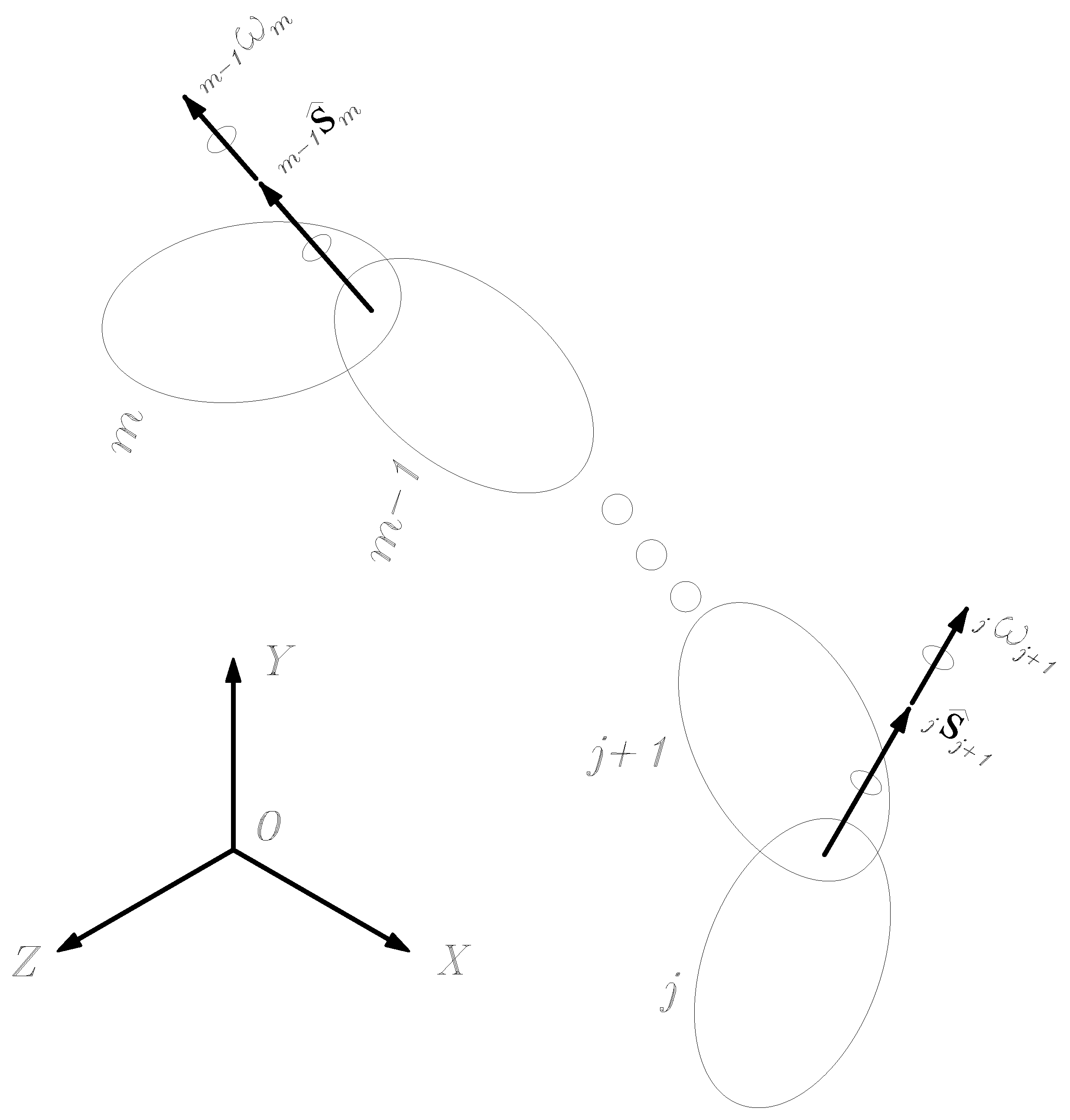
Figure 5 shows an open kinematic chain where the bodies labeled m and j are uninary links. For example, j and m would be considered as the fixed link and the end effector of a serial manipulator, respectively. Between bodies m and j, there are intermediate links forming the spinal column of the serial manipulator. The velocity state of body m as measured from body j considering point O as the reference pole is given by

$$\begin{array}{c}\hfill {}^j{\mathit{V}}_O^m={}^j{\mathit{V}}_O^{j+1}+{}^{j+1}{\mathit{V}}_O^{j+2}+\cdots +{}^{m-2}{\mathit{V}}_O^{m-1}+{}^{m-1}{\mathit{V}}_O^m\end{array}$$

(29)

Proof. 

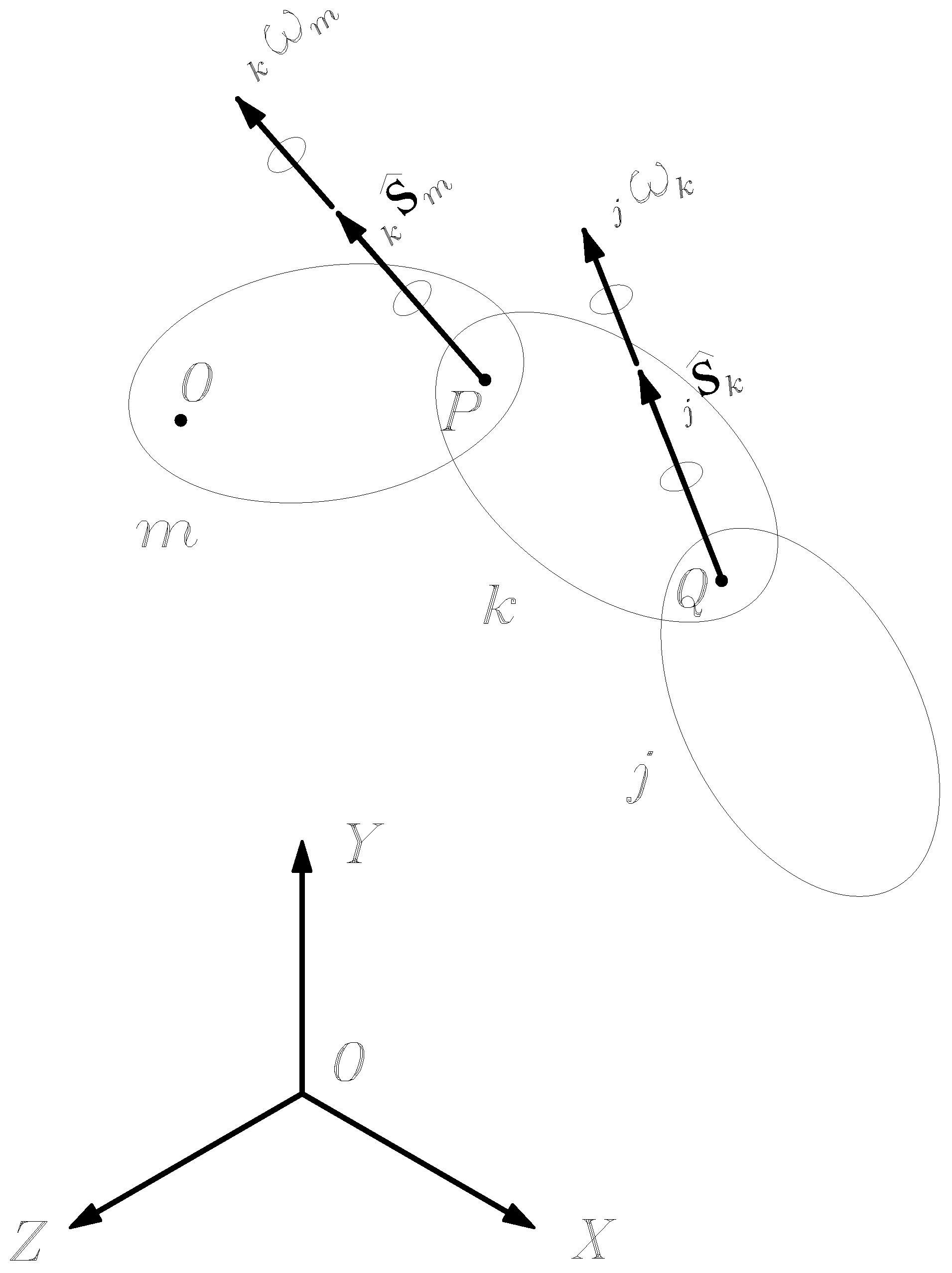
Let us consider three bodies, j, k, and m, that are serially connected by helical pairs, as shown in Figure 6. Furthermore, let us consider that $\mathit{\beta }$ is an arbitrary vector embedded in body m. Then, the time derivative of $\mathit{\beta }$ may be obtained considering the reference frames j and k as follows:

$$\begin{array}{c}\hfill \frac{{}^{j}d\mathit{\beta }}{dt}={}^j{\mathit{\omega }}^m\times \mathit{\beta },\frac{{}^{k}d\mathit{\beta }}{dt}={}^k{\mathit{\omega }}^m\times \mathit{\beta }\end{array}$$

(30)

On the other hand, to change the reference frame of the time derivative, consider that

$$\begin{array}{c}\hfill \frac{{}^{j}d\mathit{\beta }}{dt}={}^j{\mathit{\omega }}^k\times \mathit{\beta }+\frac{{}^{k}d\mathit{\beta }}{dt}\end{array}$$

(31)

Thus,

$$\begin{array}{c}\hfill \frac{{}^{j}d\mathit{\beta }}{dt}={}^j{\mathit{\omega }}^k\times \mathit{\beta }+{}^k{\mathit{\omega }}^m\times \mathit{\beta }=({}^j{\mathit{\omega }}^k+{}^k{\mathit{\omega }}^m)\times \mathit{\beta }\end{array}$$

(32)

which leads to

$$\begin{array}{c}\hfill {}^j{\mathit{\omega }}^m\times \mathit{\beta }=({}^j{\mathit{\omega }}^k+{}^k{\mathit{\omega }}^m)\times \mathit{\beta }\end{array}$$

(33)

Therefore,

$$\begin{array}{c}\hfill {}^j{\mathit{\omega }}^m={}^j{\mathit{\omega }}^k+{}^k{\mathit{\omega }}^m\end{array}$$

(34)

and assuming that $j=m-2$ and $k=m-1$, one obtains

$$\begin{array}{c}\hfill {}^{m-2}{\mathit{\omega }}^m={}^{m-2}{\mathit{\omega }}^{m-1}+{}^{m-1}{\mathit{\omega }}^m\end{array}$$

(35)

By the induction hypothesis supposes that

$$\begin{array}{c}\hfill {}^{j+1}{\mathit{\omega }}^m={}^{j+1}{\mathit{\omega }}^{j+2}+\cdots +{}^{m-2}{\mathit{\omega }}^{m-1}+{}^{m-1}{\mathit{\omega }}^m\end{array}$$

(36)

and substituting $k=j+1$ into Equation (34), we have

$$\begin{array}{c}\hfill {}^j{\mathit{\omega }}^m={}^j{\mathit{\omega }}^{j+1}+{}^{j+1}{\mathit{\omega }}^m\end{array}$$

(37)

Hence, by resorting to Equation (36), one obtains

$$\begin{array}{c}\hfill {}^j{\mathit{\omega }}^m={}^j{\mathit{\omega }}^{j+1}+{}^{j+1}{\mathit{\omega }}^{j+2}+\cdots +{}^{m-2}{\mathit{\omega }}^{m-1}+{}^{m-1}{\mathit{\omega }}^m\end{array}$$

(38)

□

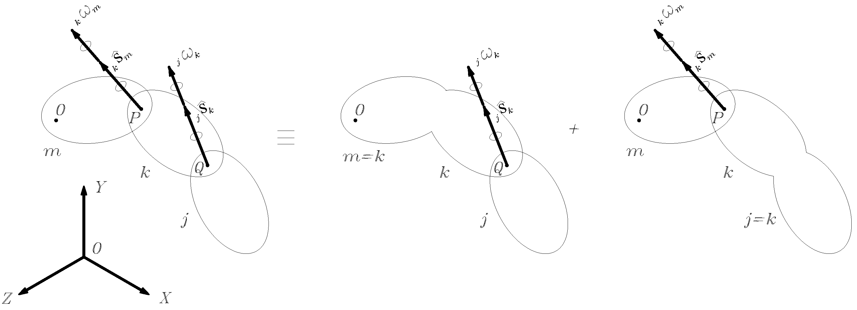
To obtain ${}^j{\mathit{v}}_O^m$, consider Figure 7. In that concern, without loss of generality the reference pole O would be precisely the origin of the reference frame $O\text{\_}XYZ$.

As shown in the second subfigure of Figure 7, the velocity vector ${}^j{\mathit{v}}_O^k$ of point O, fixed in body k as observed from body j, is given by

$$\begin{array}{c}\hfill {}^j{\mathit{v}}_O^k={}_j{h}_k{}^j{\mathit{\omega }}^k+{}^j{\mathit{\omega }}^k\times {\mathit{r}}_{O/Q}\end{array}$$

(39)

Similarly, according to the last subfigure of Figure 7, it follows that the velocity vector ${}^k{\mathit{v}}_O^m$ of point O, fixed in body m as observed from body k, is given by

$$\begin{array}{c}\hfill {}^k{\mathit{v}}_O^m={}_k{h}_m{}^k{\mathit{\omega }}^m+{}^k{\mathit{\omega }}^m\times {\mathit{r}}_{O/P}\end{array}$$

(40)

Hence, the velocity vector ${}^j{\mathit{v}}_O^m$ of point O, fixed in body body m as observed from body j, results in

$$\begin{array}{c}\hfill {}^j{\mathit{v}}_O^m={}_j{h}_k{}^j{\mathit{\omega }}^k+{}^j{\mathit{\omega }}^k\times {\mathit{r}}_{O/Q}+{}_k{h}_m{}^k{\mathit{\omega }}^m+{}^k{\mathit{\omega }}^m\times {\mathit{r}}_{O/P}\end{array}$$

(41)

or

$$\begin{array}{c}\hfill {}^j{\mathit{v}}_O^m={}^j{\mathit{v}}_O^k+{}^k{\mathit{v}}_O^m\end{array}$$

(42)

Following the trend of the angular velocity vector ${}^j{\mathit{\omega }}^m$ (see Equation (38), for the open kinematic chain of Figure 5), one obtains

$$\begin{array}{c}\hfill {}^j{\mathit{v}}_O^m={}^j{\mathit{v}}_O^{j+1}+{}^{j+1}{\mathit{v}}_O^{j+2}+\cdots +{}^{m-2}{\mathit{v}}_O^{m-1}+{}^{m-1}{\mathit{v}}_O^m\end{array}$$

(43)

Furthermore, taking into account that the velocity state ${}^j{\mathit{V}}_O^m$ is given by

$$\begin{array}{c}\hfill {}^j{\mathit{V}}_O^m=\left[\begin{array}{c}{}^j{\mathit{\omega }}^m\\ {}^j{\mathit{v}}_O^m\end{array}\right]\end{array}$$

(44)

from Equations (38) and (43), we have that

$$\begin{array}{c}\hfill {}^j{\mathit{V}}_O^m=\left[\begin{array}{c}{}^j{\mathit{\omega }}^m\\ {}^j{\mathit{v}}_O^m\end{array}\right]=\left[\begin{array}{c}{}^j{\mathit{\omega }}^{j+1}+{}^{j+1}{\mathit{\omega }}^{j+2}+\cdots +{}^{m-2}{\mathit{\omega }}^{m-1}+{}^{m-1}{\mathit{\omega }}^m\\ {}^j{\mathit{v}}_O^{j+1}+{}^{j+1}{\mathit{v}}_O^{j+2}+\cdots +{}^{m-2}{\mathit{v}}_O^{m-1}+{}^{m-1}{\mathit{v}}_O^m\end{array}\right]\end{array}$$

(45)

or

$$\begin{array}{c}\hfill {}^j{\mathit{V}}_O^m=\left[\begin{array}{c}{}^j{\mathit{\omega }}^{j+1}\\ {}^j{\mathit{v}}_O^{j+1}\end{array}\right]+\left[\begin{array}{c}{}^{j+1}{\mathit{\omega }}^{j+2}\\ {}^{j+1}{\mathit{v}}_O^{j+2}\end{array}\right]+\cdots +\left[\begin{array}{c}{}^{m-2}{\mathit{\omega }}^{m-1}\\ {}^{m-2}{\mathit{v}}_O^{m-1}\end{array}\right]+\left[\begin{array}{c}{}^{m-1}{\mathit{\omega }}^m\\ {}^{m-1}{\mathit{v}}_O^m\end{array}\right]\end{array}$$

(46)

which finally leads to Equation (29) completing the proof of Theorem 3.

It is interesting to note that Theorem 3 allows us to formulate the velocity state ${}^j{\mathit{V}}_O^m$ in terms of the infinitesimal screws of the serial kinematic chain by resorting recursively to Equation (28) as follows:

$$\begin{array}{c}\hfill {}^j{\mathit{V}}_O^m={}_j{\omega }_{j+1}{}^j{\$}^{j+1}+{}_{j+1}{\omega }_{j+2}{}^{j+1}{\$}^{j+2}+\cdots +{}_{m-2}{\omega }_{m-1}{}^{m-2}{\$}^{m-1}+{}_{m-1}{\omega }_m{}^{m-1}{\$}^m\end{array}$$

(47)

Expression (47) is one of the highlights of the theory of screws. Its introduction in the 1980s [22] marked the successful beginning of screw theory in the kinematic analysis of robotic manipulators.

2.4.2. Acceleration

The acceleration state $\mathit{A}$ of rigid body refers to the set of kinematic elements required to characterize the acceleration of a rigid body. Let m be a rigid body in general motion as observed from body j. At a glance the acceleration state of rigid body m would be considered as the time derivative of the corresponding velocity state. However, this is an erroneous assumption because the helicoidal vectorial field conditions are not satisfied with this hypothesis [18]. Brand [23] defined the acceleration state of body m as measured from body j, the six-dimensional vector ${}^j{\mathit{A}}_P^m$, as follows:

$$\begin{array}{c}\hfill {}^j{\mathit{A}}_P^m=\left[\begin{array}{c}{}^j{\mathit{\alpha }}^m\\ {\mathit{a}}_P-{}^j{\mathit{\omega }}^m\times {\mathit{v}}_P\end{array}\right]\end{array}$$

(48)

where ${}^j{\mathit{\alpha }}^m=\frac{{}^{j}d}{dt}{}^j{\mathit{\omega }}^m$ is the angular acceleration vector, while ${\mathit{a}}_P$ is the acceleration vector of point P.

$$\begin{array}{c}\hfill {}^j{\mathit{\alpha }}^m=\frac{{}^{j}d}{dt}{}^j{\mathit{\omega }}^m=\frac{{}^{j}d}{dt}{}_j{\omega }_m{}^j{\widehat{\mathit{s}}}^m={}_j{\alpha }_m{}^j{\widehat{\mathit{s}}}^m\end{array}$$

(49)

Hence

$$\begin{array}{c}\hfill {}^j{\mathit{\alpha }}^m={}_j{\alpha }_m{}^j{\widehat{\mathit{s}}}^m\end{array}$$

(50)

On the other hand, with reference to Figure 4 and Equation (23), the acceleration of point Q on the Mozzi axis is given by

$$\begin{array}{c}\hfill {\mathit{a}}_Q=\frac{{}^{j}d}{dt}{\mathit{v}}_Q=\frac{{}^{j}d}{dt}\left({}_j{\omega }_{m}h{}^j{\widehat{\mathit{s}}}^m\right)\end{array}$$

(51)

Thus,

$$\begin{array}{c}\hfill {\mathit{a}}_Q={}_j{\alpha }_{m}h{}^j{\widehat{\mathit{s}}}^m\end{array}$$

(52)

Furthermore, by resorting to elementary kinematics, the acceleration of point P can be calculated as

$$\begin{array}{c}\hfill {\mathit{a}}_P={\mathit{a}}_Q+{}^j{\mathit{\alpha }}^m\times {\mathit{r}}_{P/Q}+{}^j{\mathit{\omega }}^m\times ({}^j{\mathit{\omega }}^m\times {\mathit{r}}_{P/Q})\end{array}$$

(53)

However, ${\mathit{v}}_P={}^j{\mathit{\omega }}^m\times {\mathit{r}}_{P/Q}$. Therefore,

$$\begin{array}{c}\hfill {\mathit{a}}_P-{}^j{\mathit{\omega }}^m\times {\mathit{v}}_P={\mathit{a}}_Q+{}^j{\mathit{\alpha }}^m\times {\mathit{r}}_{P/Q}\end{array}$$

(54)

The substitution of Equations (50) and (52) into Equation (55) leads to

$$\begin{array}{c}\hfill {\mathit{a}}_P-{}^j{\mathit{\omega }}^m\times {\mathit{v}}_P={}_j{\alpha }_{m}h{}^j{\widehat{\mathit{s}}}^m+{}_j{\alpha }_m{}^j{\widehat{\mathit{s}}}^m\times {\mathit{r}}_{P/Q}\end{array}$$

(55)

or

$$\begin{array}{c}\hfill {\mathit{a}}_P-{}^j{\mathit{\omega }}^m\times {\mathit{v}}_P={}_j{\alpha }_m(h{}^j{\widehat{\mathit{s}}}^m+{}^j{\widehat{\mathit{s}}}^m\times {\mathit{r}}_{P/Q})\end{array}$$

(56)

Therefore,

$$\begin{array}{c}\hfill {\mathit{a}}_P-{}^j{\mathit{\omega }}^m\times {\mathit{v}}_P={}_j{\alpha }_m{}^j{\mathit{s}}_P^m\end{array}$$

(57)

Finally, the substitution of Equations (50) and (57) into Equation (48) yields [21]

$$\begin{array}{c}\hfill {}^j{\mathit{A}}_P^m={}_j{\alpha }_m{}^j{\$}^m\end{array}$$

(58)

Expression (58) is a confirmation of the correctness of the acceleration state of the rigid body introduced by Rico and Duffy [21], which, by the way, guarantees that the acceleration state, like the velocity state, is a twist about a screw.

Theorem 4.

Figure 5 shows an open kinematic chain where the bodies labeled m and j are unitary links. For example, j and m would be considered as the fixed link and the end effector of a serial manipulator, respectively. Between bodies m and j, there are intermediate links forming the spinal column of the serial manipulator. The acceleration state of body m as measured from body j is given by

$$\begin{array}{c}\hfill {}^j{\mathit{A}}_O^m={}^j{\mathit{A}}_O^{j+1}+{}^{j+1}{\mathit{A}}_O^{j+2}+\cdots +{}^{m-2}{\mathit{A}}_O^{m-1}+{}^{m-1}{\mathit{A}}_O^m+{}^j{\mathit{A}}_O^m+{}^j{\mathcal{A}}_O^m\end{array}$$

(59)

where ${}^j{\mathcal{A}}_O^m$ is the Coriolis-Lie vector of acceleration, which is given by

$$\begin{array}{cc}\hfill {}^j{\mathcal{A}}_O^m=& \left[\begin{array}{c}{}^j{\mathit{V}}_O^{j+1}{}^{j+1}{\mathit{V}}_O^{j+2}+{}^{j+2}{\mathit{V}}_O^{j+3}+\cdots +{}^{m-2}{\mathit{V}}_O^{m-1}+{}^{m-1}{\mathit{V}}_O^m\end{array}\right]+\hfill \\ \hfill & \left[\begin{array}{c}{}^{j+1}{\mathit{V}}_O^{j+2}{}^{j+2}{\mathit{V}}_O^{j+3}+{}^{j+3}{\mathit{V}}_O^{j+4}+\cdots +{}^{m-2}{\mathit{V}}_O^{m-1}+{}^{m-1}{\mathit{V}}_O^m\end{array}\right]+\cdots +\hfill \\ \hfill & \left[\begin{array}{c}{}^{m-2}{\mathit{V}}_O^{m-1}{}^{m-1}{\mathit{V}}_O^m\end{array}\right]\hfill \end{array}$$

(60)

Proof. 

Let us consider three bodies, j, k, and m, in relative motion; see Figure 6. The angular acceleration vector ${}^j{\mathit{\alpha }}^m$ may be obtained upon Equation (34) as follows:

$$\begin{array}{c}\hfill {}^j{\mathit{\alpha }}^m=\frac{{}^{j}d}{dt}{}^j{\mathit{\omega }}^m=\frac{{}^{j}d}{dt}({}^j{\mathit{\omega }}^k+{}^k{\mathit{\omega }}^m)=\frac{{}^{j}d}{dt}{}^j{\mathit{\omega }}^k+{}^j{\mathit{\omega }}^k\times {}^k{\mathit{\omega }}^m+\frac{{}^{k}d}{dt}{}^k{\mathit{\omega }}^m\end{array}$$

(61)

Hence,

$$\begin{array}{c}\hfill {}^j{\mathit{\alpha }}^m={}^j{\mathit{\alpha }}^k+{}^k{\mathit{\alpha }}^m+{}^j{\mathit{\omega }}^k\times {}^k{\mathit{\omega }}^m\end{array}$$

(62)

Considering that $j=m-2$ and $k=m-1$, then, one obtains that

$$\begin{array}{c}\hfill {}^{m-2}{\mathit{\alpha }}^m={}^{m-2}{\mathit{\alpha }}^{m-1}+{}^{m-1}{\mathit{\alpha }}^m+{}^{m-2}{\mathit{\omega }}^{m-1}\times {}^{m-1}{\mathit{\omega }}^m\end{array}$$

(63)

Afterwards, based on the induction hypothesis, assume that

$$\begin{array}{cc}\hfill {}^{j+1}{\mathit{\alpha }}^m=& {}^{j+1}{\mathit{\alpha }}^{j+2}+\cdots +{}^{m-2}{\mathit{\alpha }}^{m-1}+{}^{m-1}{\mathit{\alpha }}^m+{}^{j+1}{\mathit{\omega }}^{j+2}\times ({}^{j+2}{\mathit{\omega }}^{j+3}+\cdots +{}^{m-1}{\mathit{\omega }}^m)+\hfill \\ \hfill & {}^{j+2}{\mathit{\omega }}^{j+3}\times ({}^{j+3}{\mathit{\omega }}^{j+4}+\cdots +{}^{m-1}{\mathit{\omega }}^m)+\cdots +{}^{m-2}{\mathit{\omega }}^{m-1}\times {}^{m-1}{\mathit{\omega }}^m\hfill \end{array}$$

(64)

Substitution $k=j+1$ into Equation (62) yields

$$\begin{array}{c}\hfill {}^j{\mathit{\alpha }}^m={}^j{\mathit{\alpha }}^{j+1}+{}^{j+1}{\mathit{\alpha }}^m+{}^j{\mathit{\omega }}^{j+1}\times {}^{j+1}{\mathit{\omega }}^m\end{array}$$

(65)

With the substitution of Equation (64) into Equation (65), we have the result

$$\begin{array}{cc}\hfill {}^j{\mathit{\alpha }}^m=& {}^j{\mathit{\alpha }}^{j+1}+\cdots +{}^{m-2}{\mathit{\alpha }}^{m-1}+{}^{m-1}{\mathit{\alpha }}^m+{}^j{\mathit{\omega }}^{j+1}\times ({}^{j+1}{\mathit{\omega }}^{j+2}+\cdots +{}^{m-1}{\mathit{\omega }}^m)+\hfill \\ \hfill & {}^{j+1}{\mathit{\omega }}^{j+2}\times ({}^{j+2}{\mathit{\omega }}^{j+3}+\cdots +{}^{m-1}{\mathit{\omega }}^m)+\cdots +{}^{m-2}{\mathit{\omega }}^{m-1}\times {}^{m-1}{\mathit{\omega }}^m\hfill \end{array}$$

(66)

On the other hand, referring to Figure 6 and Figure 7, consider that the acceleration vector of point O is given by

$$\begin{array}{c}\hfill {}^j{\mathit{a}}_O^m={}^j{\mathit{a}}_O^k+{}^k{\mathit{a}}_O^m+2{}^j{\mathit{\omega }}^k\times {}^k{\mathit{v}}_O^m\end{array}$$

(67)

Thereafter, based on Equation (48) it follows that

$$\begin{array}{cc}\hfill {}^j{\mathit{A}}_O^m=& \left[\begin{array}{c}{}^j{\mathit{\alpha }}^m\\ {}^j{\mathit{a}}_O^m-{}^j{\mathit{\omega }}^m\times {}^j{\mathit{v}}_O^m\end{array}\right]=\left[\begin{array}{c}{}^j{\mathit{\alpha }}^k+{}^k{\mathit{\alpha }}^m+{}^j{\mathit{\omega }}^k\times {}^k{\mathit{\omega }}^m\\ {}^j{\mathit{a}}_O^k+{}^k{\mathit{a}}_O^m+2{}^j{\mathit{\omega }}^k\times {}^k{\mathit{v}}_O^m-({}^j{\mathit{\omega }}^k+{}^k{\mathit{\omega }}^m)\times ({}^j{\mathit{v}}_O^k+{}^k{\mathit{v}}_O^m)\end{array}\right]\hfill \\ \hfill =& \left[\begin{array}{c}{}^j{\mathit{\alpha }}^k\\ {}^j{\mathit{a}}_O^k-{}^j{\mathit{\omega }}^k\times {}^j{\mathit{v}}_O^k\end{array}\right]+\left[\begin{array}{c}{}^k{\mathit{\alpha }}^m\\ {}^k{\mathit{a}}_O^m-{}^k{\mathit{\omega }}^m\times {}^k{\mathit{v}}_O^m\end{array}\right]+\left[\begin{array}{c}{}^j{\mathit{\omega }}^k\times {}^k{\mathit{\omega }}^m\\ {}^j{\mathit{\omega }}^k\times {}^k{\mathit{v}}_O^m-{}^k{\mathit{\omega }}^m\times {}^j{\mathit{v}}_O^k\end{array}\right]\hfill \end{array}$$

(68)

or

$$\begin{array}{c}\hfill {}^j{\mathit{A}}_O^m={}^j{\mathit{A}}_O^k+{}^k{\mathit{A}}_O^m+\left[\begin{array}{c}{}^j{\mathit{V}}_O^k{}^k{\mathit{V}}_O^m\end{array}\right]\end{array}$$

(69)

Finally, by the induction hypothesis, one obtains Equation (59), completing the proof of Theorem 4. It is interesting to note that by resorting to Equation (58), the acceleration state ${}^j{\mathit{A}}_O^m$ may be written in screw form as follows:

$$\begin{array}{c}\hfill {}^j{\mathit{A}}_O^m={}_j{\alpha }_{j+1}{}^j{\$}^{j+1}+{}_{j+1}{\alpha }_{j+2}{}^{j+1}{\$}^{j+2}+\cdots +{}_{m-2}{\alpha }_{m-1}{}^{m-2}{\$}^{m-1}+{}_{m-1}{\alpha }_m{}^{m-1}{\$}^m+{}^j{\$a}^m\end{array}$$

(70)

where ${}^j{\$a}^m$ is given by

$$\begin{array}{cc}\hfill {}^j{\$a}^m=& \left[\begin{array}{c}{}_j{\omega }_{j+1}{}^j{\$}^{j+1}{}_{j+1}{\omega }_{j+2}{}^{j+1}{\$}^{j+2}+\cdots +{}_{m-1}{\omega }_m{}^{m-1}{\$}^m\end{array}\right]+\hfill \\ \hfill & \left[\begin{array}{c}{}_{j+1}{\omega }_{j+2}{}^{j+1}{\$}^{j+2}{}_{j+2}{\omega }_{j+3}{}^{j+2}{\$}^{j+3}+\cdots +{}_{m-1}{\omega }_m{}^{m-1}{\$}^m\end{array}\right]+\cdots +\hfill \\ \hfill & \left[\begin{array}{c}{}_{m-2}{\omega }_{m-1}{}^{m-2}{\$}^{m-1}{}_{m-1}{\omega }_m{}^{m-1}{\$}^m\end{array}\right]\hfill \end{array}$$

(71)

□

3. Symbolic Computation: Maple Sheets

In this section, Maple sheets for computing some relevant operations of the Lie algebra $se\left(3\right)$ of the Euclidean group $SE\left(3\right)$, as well as the velocity and acceleration states of rigid bodies in open kinematic chains, are reported.

Lie product between two six-dimensional vectors:

Klein form between two six-dimensional vectors:

Killing form between two six-dimensional vectors:

Velocity and acceleration states of rigid body:

4. Examples

4.1. Planar RPR Serial Manipulator

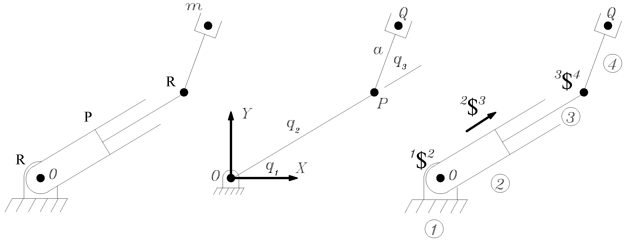
Figure 8 shows an open kinematic chain playing the role of a three-degree-of-freedom planar serial manipulator.

The base link 0 is connected to the end effector m by means of a prismatic joint P assembled between two revolute joints R. Two rotary actuators $q_1$ and $q_3$ associated with the revolute joints endowed with a linear actuator $q_2$ associated with the lonely prismatic joint are employed to control the position and orientation of the end effector m as observed from the base link 0. More specifically, $q_1$ denotes the orientation of the skirt piston with respect to the base link, $q_2$ denotes the variable length of the connecting rod including the corresponding offsets, and $q_3$ denotes the orientation of the end effector with respect to the piston. The example consists of symbolically computing the velocity and acceleration states of the end effector m as observed from the base link 0, assuming that Q is the reference pole.

Referring to Figure 8, the infinitesimal screws of the RPR serial manipulator are given by

$$\begin{array}{c}\hfill {}^1{\$}^2=\left[\begin{array}{c}{}^1{\widehat{\mathit{s}}}^2\\ {\mathit{r}}_{O/Q}\times {}^1{\widehat{\mathit{s}}}^2\end{array}\right],{}^2{\$}^3=\left[\begin{array}{c}\mathbf{0}\\ {}^2{\widehat{\mathit{s}}}^3\end{array}\right],{}^3{\$}^4=\left[\begin{array}{c}{}^3{\widehat{\mathit{s}}}^4\\ {\mathit{r}}_{P/Q}\times {}^3{\widehat{\mathit{s}}}^4\end{array}\right]\end{array}$$

(72)

where the primal parts of the screws representing the revolute joints are given by

$$\begin{array}{c}\hfill {}^1{\widehat{\mathit{s}}}^2={}^3{\widehat{\mathit{s}}}^4=\left[\begin{array}{c}0\\ 0\\ 1\end{array}\right],{}^2{\widehat{\mathit{s}}}^3=\left[\begin{array}{c}\cos q_1\\ \sin q_1\\ 0\end{array}\right]\end{array}$$

The application of the algorithm yields the following velocity and acceleration states of body 4 as measured from body 1, taking point Q as the reference pole.

$$\begin{array}{cc}\hfill {}^1{\mathit{V}}_Q^4=& \left[\begin{array}{c}0\\ \\ 0\\ \\ {}_1{\omega }_2+{}_3{\omega }_4\\ \\ -[q_2\sin q_1+a\sin (q_1+q_3)]{}_1{\omega }_2+q_2\cos q_1{}_2{\omega }_3-a\sin (q_1+q_3){}_3{\omega }_4\\ \\ [q_2\cos q_1+a\cos (q_1+q_3)]{}_1{\omega }_2+q_2\sin q_1{}_2{\omega }_3-a\cos (q_1+q_3){}_3{\omega }_4\\ \\ 0\end{array}\right]\hfill \\ \hfill {}^1{\mathit{A}}_Q^4=& \left[\begin{array}{c}0\\ \\ 0\\ \\ {}_1{\alpha }_2+{}_3{\alpha }_4\\ \\ (-q_2\sin q_1-a\sin q_1\cos q_3-a\cos q_1\sin q_3){}_1{\alpha }_2+q_2\cos q_1{}_2{\alpha }_3-\\ a(\sin q_1\cos q_3+\cos q_1\sin q_3){}_3{\alpha }_4-q_2\sin q_1{}_1{\omega }_2{}_2{\omega }_3+\\ q_2\cos q_1{}_1{\omega }_2{}_3{\omega }_4+q_2\sin q_1{}_2{\omega }_3{}_3{\omega }_4\\ \\ (q_2\cos q_1+a\cos q_1\cos q_3-a\sin q_1\sin q_3){}_1{\alpha }_2+q_2\sin q_1{}_2{\alpha }_3+\\ a(\cos q_1\cos q_3-\sin q_1\sin q_3){}_3{\alpha }_4+q_2\cos q_1{}_1{\omega }_2{}_2{\omega }_3+\\ q_2\sin q_1{}_1{\omega }_2{}_3{\omega }_4-q_2\cos q_1{}_2{\omega }_3{}_3{\omega }_4\\ \\ 0\end{array}\right]\hfill \end{array}$$

where ${}_1{\omega }_2={\dot{q}}_1$, ${}_2{\omega }_3={\dot{q}}_2$, ${}_3{\omega }_4={\dot{q}}_3$, ${}_1{\alpha }_2={\ddot{q}}_1$, ${}_2{\alpha }_3={\ddot{q}}_2$, and ${}_3{\alpha }_4={\ddot{q}}_3$.

4.2. PUMA Robot

PUMA stands for Programmable Universal Assembly Machine or Programmable Universal Manipulator Arm. This non-redundant spatial serial manipulator was developed by General Motors based on the research work of Victor Scheinman, which was supported by MIT and Stanford University. Later on, UNIMATION provided the final impulse for the inclusion of the PUMA robot in the industry. Without a doubt, the PUMA is an emblematic robot with which modern robotics manifested its intention to replicate the movement of the human body. By that time, the potential applications of the PUMA were immediately recognized in the industry, raising great expectations, and it quickly went from being a subject academic research to a practical application. In this subsection, the velocity and acceleration analyses of the PUMA robot are approached by means of the theory of screws, which is isomorphic to the Lie algebra $se\left(3\right)$ of the Euclidean group $SE\left(3\right)$ and the motor algebra of von Mises [17]. For the sake of completeness, the position analysis of the robot is included.

4.2.1. Position Analysis

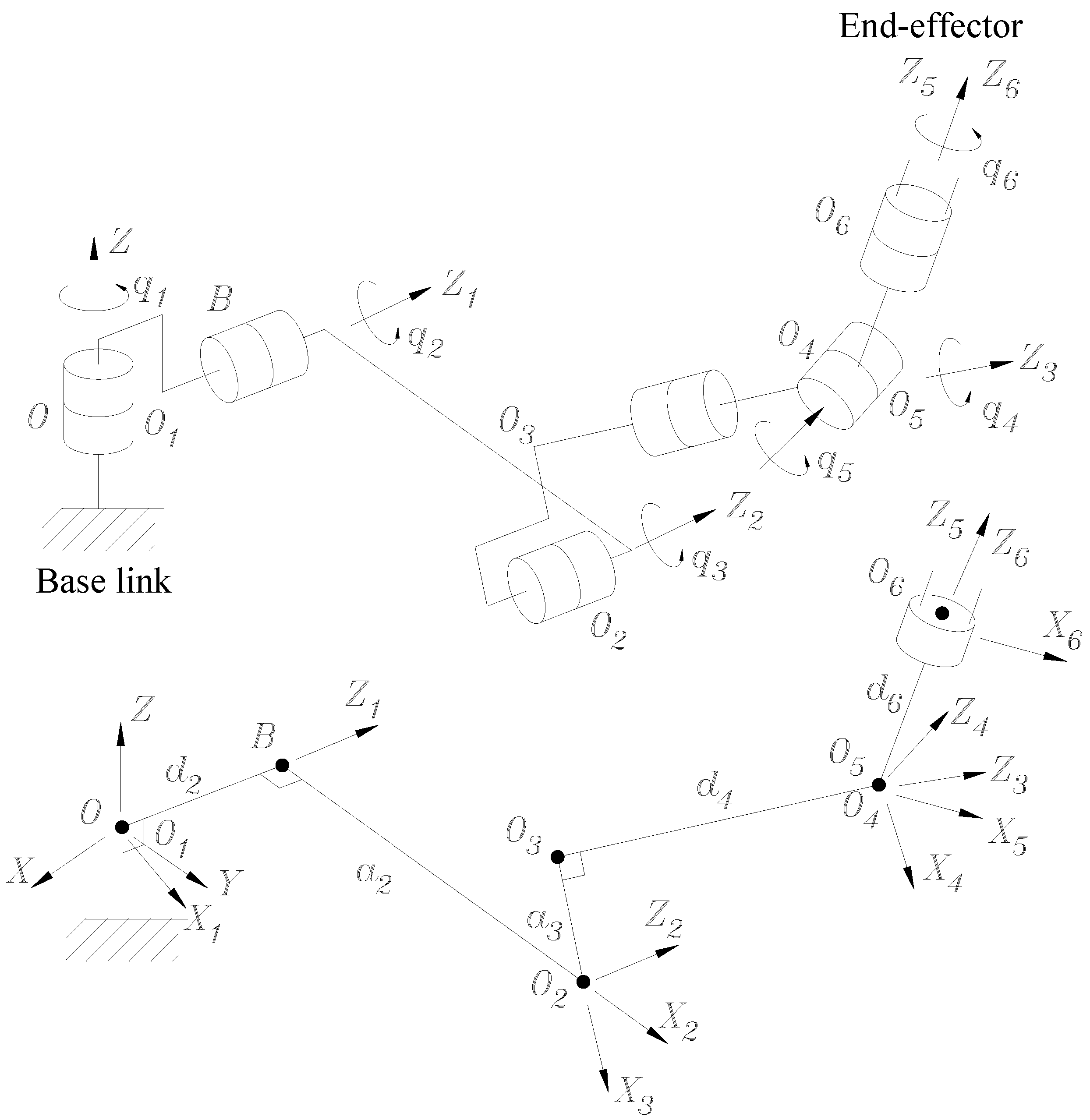
The PUMA robot is a serial manipulator with six spatial degrees of freedom composed of links articulated by means of revolute joints; see Figure 9.

The generalized coordinates of the PUMA robot are denoted by $q_i(i=1,2,3,\dots ,6)$, while the parameters, known as the Denavit–Hartenberg parameters, are notated as $a_{\ast }$ and $d_{\ast }$. The handling of several reference frames attached to different links of the robot is a natural way to solve the position analysis. With this in mind, the homogeneous transformation matrices using the Denavit–Hartenberg convention are formulated as follows

$$\begin{array}{cc}\hfill {}^0{\mathrm{T}}^1& =\left[\begin{array}{cccc}\cos q_1& 0& -\sin q_1& 0\\ \sin q_1& 0& \cos q_1& 0\\ 0& -1& 0& 0\\ 0& 0& 0& 1\end{array}\right],{}^1{\mathrm{T}}^2=\left[\begin{array}{cccc}\cos q_2& -\sin q_2& 0& a_2\cos q_2\\ \sin q_2& \cos q_2& 0& a_2\sin q_2\\ 0& 0& 1& d_2\\ 0& 0& 0& 1\end{array}\right],\hfill \\ \hfill {}^2{\mathrm{T}}^3& =\left[\begin{array}{cccc}\cos q_3& 0& \sin q_3& a_3\cos q_3\\ \sin q_3& 0& -\cos q_3& a_3\sin q_3\\ 0& 1& 0& 0\\ 0& 0& 0& 1\end{array}\right],{}^3{\mathrm{T}}^4=\left[\begin{array}{cccc}\cos q_4& 0& -\sin q_4& 0\\ \sin q_4& 0& \cos q_4& 0\\ 0& -1& 0& d_4\\ 0& 0& 0& 1\end{array}\right],\hfill \\ \hfill {}^4{\mathrm{T}}^5& =\left[\begin{array}{cccc}\cos q_5& 0& \sin q_5& 0\\ \sin q_5& 0& -\cos q_5& 0\\ 0& 1& 0& 0\\ 0& 0& 0& 1\end{array}\right],{}^5{\mathrm{T}}^6=\left[\begin{array}{cccc}\cos q_6& -\sin q_6& 0& 0\\ \sin q_6& \cos q_6& 0& 0\\ 0& 0& 1& d_6\\ 0& 0& 0& 1\end{array}\right]\hfill \end{array}$$

Thereafter, the homogeneous matrix of the end-effector m as measured from the base link 0, the matrix ${}^0{\mathrm{T}}^6$, is computed as follows:

$${}^0{\mathrm{T}}^6={}^0{\mathrm{T}}^1{}^1{\mathrm{T}}^2{}^2{\mathrm{T}}^3{}^3{\mathrm{T}}^4{}^4{\mathrm{T}}^5{}^5{\mathrm{T}}^6$$

(73)

Next, let us consider an arbitrary point Q of the end effector m. The coordinates $(Q_X,Q_Y.Q_Z)$ of point Q expressed in the fixed reference frame $O\text{\_}XYZ$ are obtained with the coordinates $(Q_{X_6},Q_{Y_6},Q_{Z_6})$ of the same point Q but expressed in the reference frame $O_6{X}_6{Y}_6{Z}_6$ as follows:

$$\begin{array}{c}\hfill \left[\begin{array}{c}{X}_Q\\ Y_Q\\ Z_Q\\ 1\end{array}\right]={}^0{\mathrm{T}}^6\left[\begin{array}{c}{x}_Q\\ y_Q\\ z_Q\\ 1\end{array}\right]\end{array}$$

(74)

4.2.2. Velocity Analysis

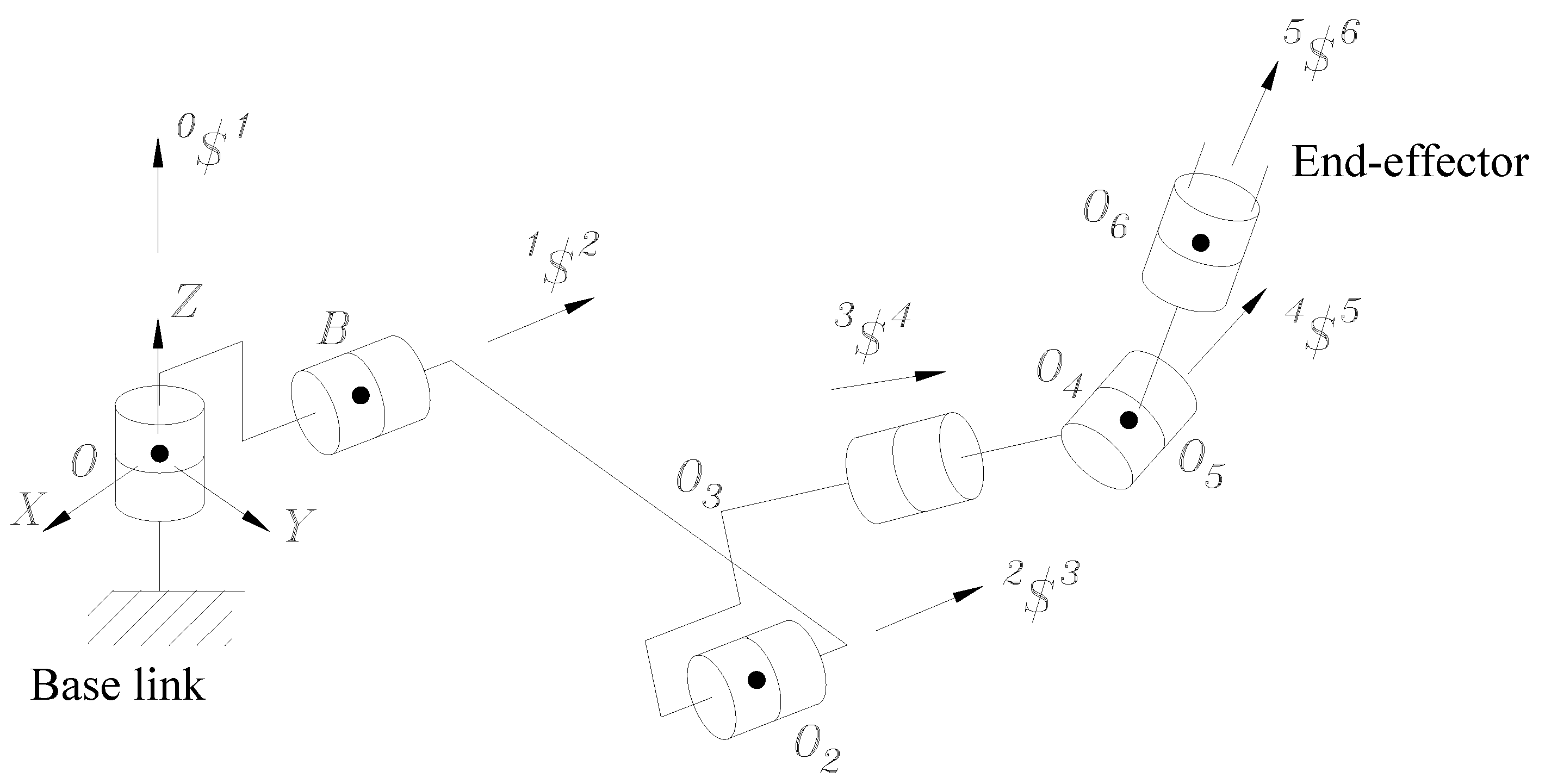
To approach the velocity analysis, Figure 10 shows the infinitesimal screws associated with the revolute joints of the PUMA robot.

Let $\mathit{\omega }={\omega }_X\widehat{\mathit{i}}+{\omega }_Y\widehat{\mathit{j}}+{\omega }_Z\widehat{\mathit{k}}$ be the angular velocity vector of the end effector, link $m=6$, as observed from the base link 0. Moreover, let ${\mathit{v}}_{O_6}=v_X\widehat{\mathit{i}}+v_Y\widehat{\mathit{j}}+v_Z\widehat{\mathit{k}}$ be the velocity vector of point $O_6$ of body 6 expressed in the global reference frame $O\text{\_}XYZ$, where the point $O_6$ is the origin of the reference frame attached to the end effector m. The velocity state ${}^0{\mathit{V}}_{O_6}^6$ of the end effector as measured from the base link may be written in matrix form as follows:

$${}^0{\mathit{V}}_{O_6}^6=\left[\begin{array}{c}{\omega }_X\\ {\omega }_Z\\ {\omega }_Z\\ v_X\\ v_Y\\ v_Z\end{array}\right]$$

(75)

where point $O_6$ is the reference pole. Moreover, the velocity state ${}^0{\mathit{V}}_{O_6}^6$ may be written in screw form as follows:

$${\dot{q}}_1{}^0{\$}^1+{\dot{q}}_2{}^1{\$}^2+{\dot{q}}_3{}^2{\$}^3+{\dot{q}}_4{}^3{\$}^4+{\dot{q}}_5{}^4{\$}^5+{\dot{q}}_6{}^5{\$}^6={}^0{\mathit{V}}_{O_6}^6$$

(76)

where the infinitesimal screws are given by

$$\begin{array}{cc}\hfill & {}^0{\$}^1=\left[\begin{array}{c}\widehat{\mathit{k}}\\ \widehat{\mathit{k}}\times {\mathit{r}}_{O_6/O}\end{array}\right],{}^1{\$}^2=\left[\begin{array}{c}{\widehat{\mathit{r}}}_{B/O}\\ {\widehat{\mathit{r}}}_{B/O}\times {\mathit{r}}_{O_6/O}\end{array}\right],{}^2{\$}^3=\left[\begin{array}{c}{\widehat{\mathit{r}}}_{B/O}\\ {\widehat{\mathit{r}}}_{B/O}\times {\mathit{r}}_{O_6/O_2}\end{array}\right],\hfill \\ \hfill & {}^3{\$}^4=\left[\begin{array}{c}{\widehat{\mathit{r}}}_{O_4/O_3}\\ {\widehat{\mathit{r}}}_{O_4/O_3}\times {\mathit{r}}_{O_6/O_4}\end{array}\right],{}^4{\$}^5=\left[\begin{array}{c}\widehat{({\mathit{r}}_{O_6/O_4}\times {\mathit{r}}_{O_4/O_3})}\\ \widehat{({\mathit{r}}_{O_6/O_4}\times {\mathit{r}}_{O_4/O_3})}\times {\mathit{r}}_{O_6/O_4}\end{array}\right],{}^5{\$}^6=\left[\begin{array}{c}{\widehat{\mathit{r}}}_{O_6/O_4}\\ \mathbf{0}\end{array}\right]\hfill \end{array}$$

and ${\widehat{\mathit{r}}}_{O_m/O_n}$ is a unitary vector parallel to ${\mathit{r}}_{O_m/O_n}$.

Expression (76) may be written in a matrix vector form as follows

$$\mathrm{J}{\mathrm{Q}}_{\mathrm{v}}={\mathit{V}}_{O_6}$$

(77)

where $\mathrm{J}$ is the Jacobian matrix of the manipulator, which is given by

$$\mathrm{J}=\left[\begin{array}{cccccc}{}^0{\$}^1& {}^1{\$}^2& {}^2{\$}^3& {}^3{\$}^4& {}^4{\$}^5& {}^5{\$}^6\end{array}\right]$$

(78)

On the other hand, ${\mathrm{Q}}_{\mathrm{v}}={\left[\begin{array}{cccccc}{\dot{q}}_1& \dot{q_2}& {\dot{q}}_3& {\dot{q}}_4& {\dot{q}}_5& {\dot{q}}_6\end{array}\right]}^T$ is the first-order active matrix of the PUMA robot.

Expression (78) is the input–output equation of velocity of the PUMA robot and is valid for both the inverse and the direct velocity analyses of the robot manipulator.

4.2.3. Acceleration Analysis

Let $\mathit{\alpha }={\alpha }_X\widehat{\mathit{i}}+{\alpha }_Y\widehat{\mathit{j}}+{\alpha }_Z\widehat{\mathit{k}}$ be the angular acceleration vector of the end effector $m=6$ as observed from the fixed link 0. Moreover, let ${\mathit{a}}_{O_6}=a_X\widehat{\mathit{i}}+a_Y\widehat{\mathit{j}}+a_Z\widehat{\mathit{k}}$ be the acceleration vector of point $O_6$. The acceleration state of the end effector, as observed from the base link, taking point $O_6$ as the reference pole as given by

$${\mathit{A}}_{O_6}=\left[\begin{array}{c}\mathit{\alpha }\\ {\mathit{a}}_{O_6}-\mathit{\omega }\times {\mathit{v}}_{O_6}\end{array}\right]$$

(79)

Moreover, the acceleration equation in screw form of the PUMA robot may be written as follows:

$${\ddot{q}}_1{}^0{\$}^1+{\ddot{q}}_2{}^1{\$}^2+{\ddot{q}}_3{}^2{\$}^3+{\ddot{q}}_4{}^3{\$}^4+{\ddot{q}}_5{}^4{\$}^5+{\ddot{q}}_6{}^5{\$}^6+\$a={}^0{\mathit{A}}_{O_6}^6$$

(80)

where

$$\begin{array}{cc}\hfill \$a& =\left[\begin{array}{c}{\dot{q}}_1{}^0{\$}^1{\dot{q}}_2{}^1{\$}^2+{\dot{q}}_3{}^2{\$}^3+{\dot{q}}_4{}^3{\$}^4+{\dot{q}}_5{}^4{\$}^5+{\dot{q}}_6{}^5{\$}^6\end{array}\right]+\hfill \\ \hfill & \left[\begin{array}{c}{\dot{q}}_2{}^1{\$}^2{\dot{q}}_3{}^2{\$}^3+{\dot{q}}_4{}^3{\$}^4+{\dot{q}}_5{}^4{\$}^5+{\dot{q}}_6{}^5{\$}^6\end{array}\right]+\left[\begin{array}{c}{\dot{q}}_3{}^2{\$}^3{\dot{q}}_4{}^3{\$}^4+{\dot{q}}_5{}^4{\$}^5+{\dot{q}}_6{}^5{\$}^6\end{array}\right]+\hfill \\ \hfill & \left[\begin{array}{c}{\dot{q}}_4{}^3{\$}^4{\dot{q}}_5{}^4{\$}^5+{\dot{q}}_6{}^5{\$}^6\end{array}\right]+\left[\begin{array}{c}{\dot{q}}_5{}^4{\$}^5{\dot{q}}_6{}^5{\$}^6\end{array}\right]\hfill \end{array}$$

Expression (80) may be written in matrix vector form by introducing the Jacobian matrix $\mathrm{J}$ of the velocity analysis as follows:

$$\mathrm{J}{\mathrm{Q}}_{\mathrm{a}}+\$a={\mathit{A}}_{O_6}$$

(81)

where ${\mathrm{Q}}_{\mathrm{a}}={\left[\begin{array}{cccccc}{\ddot{q}}_1& {\ddot{q}}_2& {\ddot{q}}_3& {\ddot{q}}_4& {\ddot{q}}_5& {\ddot{q}}_6\end{array}\right]}^T$ is the active acceleration matrix of the manipulator, which is formed by the generalized accelerations of the robot.

4.2.4. Numerical Application

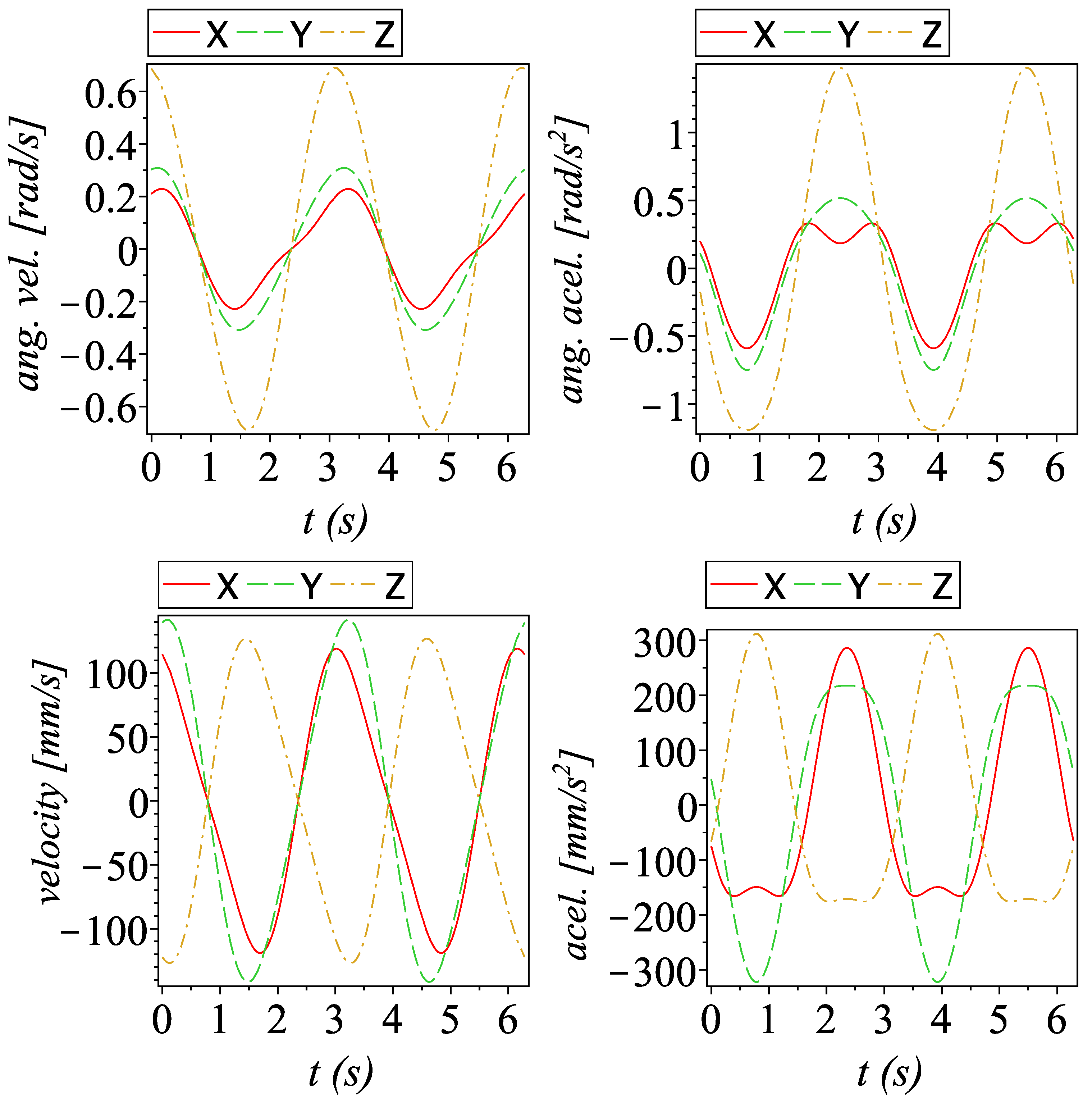
For this numerical case, let us consider the Denavit–Hartenberg parameters for a standard PUMA manipulator (Figure 9) shown in the

Table 1. Denavit–Hartenberg parameters of the PUMA robot.

Link Offset [mm]	Joint Angle	Link Length [mm]	Twist Angle [rad]
$d_1=0$	${\theta }_1=q_1$	$a_1=0$	${\alpha }_1=\frac{\pi }{2}$
$d_2=144.09$	${\theta }_2=q_2$	$a_2=431.8$	${\alpha }_2=0$
$d_3=0$	${\theta }_3=q_3$	$a_3=-20.32$	${\alpha }_3=-\frac{\pi }{2}$
$d_4=433.07$	${\theta }_4=q_4$	$a_4=0$	${\alpha }_4=\frac{\pi }{2}$
$d_5=0$	${\theta }_5=q_5$	$a_5=0$	${\alpha }_4=\frac{\pi }{2}$
$d_6=56.25$	${\theta }_6=q_6$	$a_6=0$	${\alpha }_6=0$

. On the other hand, let us consider that in the reference configuration, all the generalized coordinates of the robot are given by ${10}^{\circ }$. Furthermore, from its reference configuration, the generalized coordinates of the PUMA manipulator follow periodic functions given by $q_1=0.2\sin \left(t\right)$ [rad], $q_2=0.15\sin \left(t\right)$ [rad], $q_3=0.25\sin \left(t\right)$ [rad], $q_4=0.25\sin \left(t\right)$ [rad], $q_5=0.15\sin \left(t\right)$ [rad] and $q_6=0.3\sin \left(t\right)$ [rad], where $0\le t\le 2\pi$ [s]. With these data, we must compute the time history of the direct kinematics of the PUMA robot. The relevant resulting plots of the numerical example are shown in Figure 11.

5. Conclusions

This work presents an application of the Lie algebra $se\left(3\right)$ of the Euclidean group $SE\left(3\right)$, which is isomorphic to the theory of screws and the motor algebra, to the infinitesimal kinematics of serial manipulators. The Lie algebra, as is shown in this contribution, has been consolidated as a highly efficient mathematical tool in the analysis and synthesis of robotic manipulators. The algorithm presented allows us to symbolically compute the velocity and acceleration characteristics of the end effector of serial manipulators. In the case of complex serial manipulators, numerical computations are preferred, owing to the generation of expressions with long terms. To exemplify the presented methodology, two serial manipulators are analysed: (1) a three-dof planar serial manipulator, (2) the six-dof PUMA robot.

These procedures can be extended without significant effort to higher-order analyses such as the jerk and jounce. The fact that the screw algebra, which is isomorphic to the Lie algebra $se\left(3\right)$, has been reported and successfully tested in the analysis of robotic manipulators in previous works proves its undoubted usefulness and correctness. Unlike other algebras, the screw algebra has demonstrated its applicability and versatility in higher-order analyses, a real obstacle for other algebras such as the quaternion algebra, among others. Now, the task is to search for areas of opportunity dealing with practical applications. These applications may also require the use of hybrid methods for complex kinematic architectures, for example, in [24], where the positional analysis of a complex parallel platform is investigated by combining the well-known Newton–Raphson algorithm with methods based on homotopic continuation. In that regard, the Maple sheets provided in this work are sufficiently readable so that a non-expert user can apply them without substantial problems in specific robot manipulators. However, especially in problems where it is not possible to generate closed-form solutions, it becomes necessariy to resort to numerical methods.

References

- Ball, R.S. A Treatise on the Theory of Screws; Cambridge University Press: Cambridge, UK, 1900; reprinted 1998. [Google Scholar]
- Hunt, K.H. Kinematic Geometry of Mechanisms; Oxford University Press: New York, NY, USA, 1978. [Google Scholar]
- Phillips, J. Freedom in Machinery: Introducing Screw Theory; Cambridge University Press: Cambridge, UK, 1984; Volume 1. [Google Scholar]
- Karger, A. Singularity analysis of serial robot-manipulators. ASME Mech. Des. 1996, 118, 520–525. [Google Scholar] [CrossRef]
- Müller, A. Higher derivatives of the kinematic mapping and some applications. Mech. Mach. Theory 2014, 76, 70–85. [Google Scholar] [CrossRef]
- Wu, Y.; Carricato, M. Identification and geometric characterization of Lie triple screw systems and their exponential images. Mech. Mach. Theory 2017, 107, 305–323. [Google Scholar] [CrossRef]
- Zhang, L.; Zhao, Y.; Zhao, T. Fundamental equation of mechanism kinematic geometry: Mapping curve in se(3) to counterpart in SE(3). Mech. Mach. Theory 2020, 146, 103732. [Google Scholar] [CrossRef]
- Sanchez-Garcia, A.J.; Rico, J.M.; Cervantes-Sanchez, J.J.; Lopez-Custodio, P.C. A mobility determination method for parallel platforms based on the Lie algebra of SE(3) and Its Subspaces. ASME J. Mech. Robot. 2021, 13, 031015. [Google Scholar] [CrossRef]
- Chen, J.; Huang, Z.; Tian, Q. A multisymplectic Lie algebra variational integrator for flexible multibody dynamics on the special Euclidean group SE(3). Mech. Mach. Theory 2022, 174, 104918. [Google Scholar] [CrossRef]
- Hassani, H.; Avazzadeh, Z.; Agarwal, P.; Ebadi, M.J.; Eshkaftaki, A.B. Generalized Bernoulli—Laguerre Polynomials: Applications in Coupled Nonlinear System of Variable-Order Fractional PDEs. J. Optim. Theory Appl. 2024, 200, 371–393. [Google Scholar] [CrossRef]
- Avazzadeh, Z.; Hassani, H.; Ebadi, M.J.; Bayati Eshkaftaki, A.; Hendy, A.S. An optimization method for solving a general class of the inverse system of nonlinear fractional order PDEs. Int. J. Comput. Math. 2024, 101, 138–153. [Google Scholar] [CrossRef]
- Hodge, W.V.D.; Pedoe, D. Methods of Algebraic Geometry; Cambridge University Press: Cambridge, UK, 1994; Volume 1. [Google Scholar]
- Mason, M.T. Mechanics of Robotic Manipulation; MIT Press: Cambridge, MA, USA, 2001. [Google Scholar]
- Palais, B.; Palais, R.; Rodi, S. A Disorienting Look at Euler’s Theorem on the Axis of a Rotation. Am. Math. Mon. 2009, 116, 892–909. [Google Scholar] [CrossRef]
- Chasles, M. Note sur les propriétés générales du système de deux corps semblables entr’eux. Bull. Sci. Math. Astron. Phys. Chim. 1830, 4, 321–326. [Google Scholar]
- Mozzi, G. Discorso Matematico Sopra il Rotamento Momentaneo Dei Corpi; Nella Stamperia di Donato Campo: Campo, Italy, 1763. [Google Scholar]
- von Mises, R. Motorrechnung; ein neues Hilfsmittel der Mechanik. ZAMM 1924, 4, 155–181. [Google Scholar] [CrossRef]
- Gallardo, J.; Rico, J.M. Screw theory and helicoidal fields. In Proceedings of the ASME 25th Biennial Mechanisms Conference, Atlanta, GA, USA, 13–16 September 1998. Paper DETC98/MECH-5893. [Google Scholar]
- Gallardo-Alvarado, J. Análisis Cinemáticos de Orden Superior de Cadenas Espaciales, Mediante el Álgebra de Tornillos, y sus Aplicaciones. Doctoral Dissertation, Instituto Tecnológico de la Laguna, Torreón, México, April 1999. (In Spanish). [Google Scholar]
- Valderrama-Rodríguez, J.I.; Rico, J.M.; Cervantes-Sánchez, J.J. A general method for the determination of the instantaneous screw axes of one-degree-of-freedom spatial mechanisms. Mech. Sci. 2020, 11, 91–99. [Google Scholar] [CrossRef]
- Rico-Martinez, J.M.; Duffy, J. An application of screw algebra to the acceleration analysis of serial chains. Mech. Mach. Theory 1996, 31, 445–457. [Google Scholar] [CrossRef]
- Sugimoto, K.; Duffy, J. Application of linear algebra to screw systems. Mech. Mach. Theory 1982, 17, 73–83. [Google Scholar] [CrossRef]
- Brand, L. Vector and Tensor Analysis; John Wiley & Sons: Hoboken, NJ, USA, 1947. [Google Scholar]
- Gallardo-Alvarado, J.; Garcia-Murillo, M.A.; Aguilera-Camacho, L.D.; Alcaraz-Caracheo, L.A.; Sandoval-Castro, X.Y. An approach to solving the forward kinematics of the 5-RPUR (3T2R) parallel manipulator. J. Mech. Sci. Technol. 2023, 37, 1443–1453. [Google Scholar] [CrossRef]
Disclaimer/Publisher’s Note: The statements, opinions and data contained in all publications are solely those of the individual author(s) and contributor(s) and not of MDPI and/or the editor(s). MDPI and/or the editor(s) disclaim responsibility for any injury to people or property resulting from any ideas, methods, instructions or products referred to in the content. |
© 2024 by the authors. Licensee MDPI, Basel, Switzerland. This article is an open access article distributed under the terms and conditions of the Creative Commons Attribution (CC BY) license (https://creativecommons.org/licenses/by/4.0/).