Abstract
Federated learning facilitates the training of global models in a distributed manner without requiring the sharing of raw data. This paper introduces two novel symmetric Alternating Direction Method of Multipliers (ADMM) algorithms for federated learning. The two algorithms utilize a convex combination of current local and global variables to generate relaxed steps to improve computational efficiency. They also integrate two dual-update steps with varying relaxation factors into the ADMM framework to boost the accuracy and the convergence rate. Another key feature is the use of weak parametric assumptions to enhance computational feasibility. Furthermore, the global update in the second algorithm occurs only at certain steps (e.g., at steps that are a multiple of a pre-defined integer) to improve communication efficiency. Theoretical analysis demonstrates linear convergence under reasonable conditions, and experimental results confirm the superior convergence and heightened efficiency of the proposed algorithms compared to existing methodologies.
Keywords:
federated learning; relaxed method; symmetric alternating direction method of multipliers; linear convergence MSC:
90-10
1. Introduction
Federated learning serves as a widely adopted distributed machine learning methodology that has garnered substantial interest in recent years due to its effectiveness in addressing issues related to data privacy, security, and the accessibility of heterogeneous data [1,2,3]. This methodology has been employed extensively in various domains, such as health care [4] (Yang et al., 2019), finance [5] (Liu et al., 2021), the Internet of Things (IoT) [6] (Zeng et al., 2023), and intelligent transportation [7,8] (Manias et al., 2021). By providing solutions for data security and compliance, federated learning facilitates improved utilization of decentralized data and enhances the performance and efficiency of machine learning models. As a contemporary research hot spot, federated learning’s significance spans beyond boosting performance of machine learning models, extending to the safeguarding of data privacy, economizing computational resources, and supporting heterogeneous devices.
1.1. Related Work
(a) Improving computational efficiency and accuracy.
Each node independently addresses local optimization sub-problems in federated learning. Early research [6,9,10] used a strategy of splitting the computation across multiple devices for local optimization, although shortcomings persist regarding computational efficiency and accuracy. The Alternating Direction Method of Multipliers (ADMM), as a distributed method, has been used to solve many optimization problems due to its simplicity and efficiency. In federated learning, there are two types of ADMM available, namely exact [11] and inexact [12] ADMM. The former requires the clients to update the parameters by solving the sub-problems accurately, thereby increasing the computational burden [12,13,14,15,16,17]. The latter updates the parameters by solving sub-problems approximately, which reduces the computational complexity for clients [18,19,20,21]. However, these algorithms implement a single dual-update step per iteration and necessitate relatively stringent assumptions with respect to the parameters to ensure convergence properties.
(b) Saving computing resources. In distributed learning, local clients and the central server engage in frequent, often inefficient communication. Thus, extensive research efforts focus on devising algorithms to minimize the number of communication rounds. The stochastic gradient descent method, which aggregates in a cyclic fashion, is a widely used approach [22,23,24,25,26,27] that has demonstrated promising results in reducing the number of communication rounds. To further alleviate the burden of communication rounds, McMahan et al. [6,28,29] introduced the Federated Averaging Algorithm (FedAvg) and its improved variants. These algorithms minimize communications by performing local iterations multiple times before periodically conducting global aggregation. Li et al. [30] further refined the FedAvg method by introducing the Federated Proximal (FedProx) algorithm, allowing available device-based system resources to perform varying amounts of local work before aggregating partial solutions. Both FedAvg and FedProx have seen extensive application in distributed learning.
1.2. Our Contribution
The main contributions of this paper include the introduction of two federated learning algorithms based on Symmetric ADMM with Relaxed Step (Fed-RSADMM; see Algorithms 2 and 3), characterized as follows:
(I) Relaxed step. In contrast to the conventional ADMM, the presented algorithms employ a convex combination of the current local and global variables to generate the relaxed steps.
(II) We integrate two dual-update steps into the ADMM framework to construct a symmetric ADMM algorithm with varying relaxation factors, which is different from the general ADMM.
(III) Differing from conventional algorithmic assumptions, only simple assumptions are made with respect to the parameters.
1.3. Organization
This paper is organized as follows. In the next section, we provide the symbolic definitions and some common mathematical definitions that are used in this paper. In Section 3, we present the Fed-RSADMM and FedAvg-RSADMM algorithms, then prove their convergence. In Section 4, we design some comparative numerical experiments to illustrate the performance of our two proposed algorithms. The conclusions of this paper are presented in Section 5.
2. Preliminaries
The present section introduces some notations and definitions employed in this paper.
2.1. Notations
denotes the n-dimensional Euclidean space, , and denotes the Euclidean norm. Let the set and the point . If S is non-empty, the distance from point x to set S is denoted as . When , let .
Definition 1
(Lipschitz continuity). In mathematics, a function () is said to be L-Lipschitz continuous (or simply L-Lipschitz) if, for any , one has
where denotes the Euclidean norm.
If the function (f) is continuously differentiable and its gradient () is L-Lipschitz continuous, then we have
Definition 2.
Let the function be normally lower semicontinuous. The authors of [31] provided the following definitions:
- (I)
- The Frechet subdifferential of f at is denoted asand when , .
- (II)
- The limiting subdifferential of f at is denoted asand assuming that is a minimal-value point of f, then . If , then x is said to be a stable point of f, and the set of stable points of f is denoted as .
The proximal operator of a normal closed, convex function f at is defined as follows [32]:
where denotes the Euclidean norm.
2.2. Loss Function
A machine learning model encompasses a set of parameters that are refined based on the training data. Typically, the training data samples include the following two components: input features represented as vectors () and desired outputs known as output labels (). Each model is equipped with a loss function defined on its parameter vector (x) for each data sample. The loss function records the model error in the training data. The learning process aims to minimize this loss function over a set of training data samples (). For each data sample, the loss function is designated as or abbreviated to for convenience.
Table 1 [33,34,35,36] summarizes loss functions for popular machine learning models. For convenience, suppose there are m edge nodes and that the local datasets are . For each dataset () at node i, the loss function of the set of data samples at that node is

Table 1.
Loss functions for some models.
We define , where denotes the size of set , i.e.,
The global loss function of all distributed datasets is defined as
2.3. Symmetric ADMM
The following convex minimization model with linear constraints and a separable objective function is considered.
where and . Such divisible convex optimization problems can be solved by using the ADMM algorithm. The augmented Lagrangian function for the above optimization problem is expressed as follows.
where is the penalty parameter and u is the Lagrange multiplier. ADMM follows the following update process [37]:
Based on the Peaceman–Rachford splitting method [38], symmetric ADMM (S-ADMM) was proposed to solve (9). The iterative process is expressed as follows:
2.4. Federated Learning
Suppose we have m local nodes, each with a local dataset (). Each node has a local total loss () as a lower-bounded function. The global loss function can, therefore, be derived as
where are positive weights and satisfy
The goal of federated learning is to minimize the loss function at the central node to obtain the optimal parameter (), which can be described as the following problem:
By introducing the auxiliary variable (y) and adding the constraint of , the original problem can be rewritten in the following form:
Based on the above optimization problem, the conventional federated learning Algorithm 1 can be summarized in the following form [39]:
| Algorithm 1 Federated Learning |
|
To implement the algorithms proposed in this paper, we construct the augmented Lagrangian function for problem (14). The augmented Lagrangian function of (14) is
where , , , and
where are the Lagrange multipliers and are the penalty parameters.
2.5. Stationary Points
Here, we present the optimality condition for problem (14).
Definition 3.
Point is a stationary point of problem (14) and satisfies the following conditions:
Point is deemed a stationary point of problem (14) if it satisfies the following condition:
One can readily observe that any local optimal solution satisfies (17), and if each is a convex function, a point fulfilling (18) constitutes a globally optimal solution.
Based on the definition of the proximal operator and Definition 3, we obtain the following lemma.
Lemma 1
([39,40]). Suppose that are properly convex lower semicontinuous functions. Then, solving problem (15) reduces to a zero point of
where for any given positive constant. For , . Thus, can be used to measure the distance between point p and stable set .
Now, we provide the following lemma for , which is important for Remark 2 and Lemma 5 in Section 3.
Lemma 2
([39,40]). Suppose that are properly convex and lower semicontinuous. If p is not a stable point of and , then
and
3. Symmetric ADMM-Based Federated Learning with a Relaxed Step and Convergence
Based on the above augmented Lagrangian functions, in this section, we construct two symmetric ADMM-based federated learning algorithms, the first of which is Fed-RSADMM, which utilizes the federated learning framework and symmetric ADMM with a relaxed step (RSADMM). The second is FedAvg-RSADMM, based on Fed-RSADMM, which allows local clients to update multiple times, then upload their parameters to the central server.
3.1. Fed-RSADMM
Given an original dataset comprising m nodes, the local parameter for the -th node is set as , and data for the -th node is assigned as . The specific algorithmic workflow proceeds as follows (Algorithm 2).
| Algorithm 2 Fed-RSADMM |
|
Remark 1.
In Algorithm 2, subproblem (23) can be solved by the following equation:
where
Compared to traditional federated learning, we adopt the update methods outlined in (23) and (27) for the global parametersinstead of using the average of all local parameters, denoted as . In contrast to the symmetric ADMM algorithm, we introduce a relaxation step to accelerate the convergence rate [19].
3.2. FedAvg-RSADMM
The communications in FedAvg-RSADMM only occur when , where is a predefined positive integer. To facilitate local updates in Algorithm 2, an auxiliary variable () is introduced, where . It can be readily observed that if , then , and when , then , i.e.,
This approach decreases the number of communication rounds (e.g., parameter feedback and parameter upload), resulting in substantial cost savings with a convergence rate of , where K is the number of iterations. A convex combination between local and global variables is used to formulate the relaxed step, which is then employed to perform the parameter update. The corresponding Algorithm 3 proceeds as follows.
| Algorithm 3 FedAvg-RSADMM |
|
3.3. Convergence
In this section, we only provide the corresponding convergence lemmas and theorem for Algorithm 2, as those for Algorithm 3 follow a similar process. The following assumption is important for the proof.
Assumption 1.
- (a)
- The function is lower semi-continuous.
- (b)
- The function , is continuous and has the same L-Lipschitz continuous gradient.
- (c)
- The parameters in the algorithm satisfy the following:The penalty parameter () complies with the following:where , .
- (d)
- The datasets of all devices are independently and identically distributed (i.i.d).
We first prove the decreasing property of the sequence; these properties enable us to obtain Lemma 4, which, together with the optimality conditions, shows the convergence of the sequence.
Lemma 3.
Assuming that Assumption 1 holds, there exist and such that
Then, the sequence is monotonically decreasing, where m is a finite constant.
Lemma 4.
Assuming assumption A holds and is bounded, then
Theorem 1 establishes the subsequence convergence property of the iterative sequence generated by Algorithm 2.
Theorem 1
(Subsequence Convergence). Assuming the conditions in Lemma 4 are met, the set of accumulation points of the sequence is denoted as Ω. Then, the following conclusions hold:
- (1)
- Ω is a non-empty compact set, and as ;
- (2)
- .
3.4. Linear Convergence Rate
To obtain the local linear convergence rates of sequences {} and {} generated by Algorithm 2, the following results require that functions be convex. We also make the following assumptions:
Assumption 2.
For any , there exist and such that and , which implies
Remark 2.
According to Lemma 1, the expression for is
According to Lemma 2, for any given , we have
Thus, Assumption 2, we can also set , where and .
Assumption 3.
For any given and , there exists such that when , holds.
To prove the convergence rate, we also need Lemma 5.
Lemma 5.
Suppose Assumption 1 holds and the functions are convex; then, there exists such that
We have shown that Algorithm 2 converges. Now, we would like to see how fast this convergence is based on Lemma 5, as expressed by Theorems 3 and 4.
Theorem 2.
Suppose Assumptions 1 and 2, and the conditions in Lemma 4 hold and the that functions are convex; then, the following conclusions are valid:
- (1)
- ;
- (2)
- For any given and , there exists a positive integer () such that
- (3)
- The {} sequence is Q-linearly convergent.
Theorem 3.
Assuming the conditions in Theorem 2 hold, the sequence converges to with an R-linear convergence rate.
See the proofs of Lemmas 3 and 4, and Theorem 1, as well as Lemma 5, Theorems 2 and 3, in Appendix A.
4. Numerical Experiment
In this section, the performances of Algorithms 2 and 3 are demonstrated by two numerical arithmetic examples, namely linear regression and logistic regression, respectively. All numerical experiments were conducted on a laptop computer with 16 GB of RAM and an Intel(R) Core(TM) i5-12500H 2.3 GHz CPU, using MATLAB (R2021a) for implementation.
4.1. Testing Examples
In our examples, each local client is designated with its own objective function (, where m signifies the number of client nodes). Subsequently, every client generates random datasets ( and ). In these datasets, represents the feature data of dimension d, whereas denotes the label data of dimension 1.
Regarding Algorithms 2 and 3, we establish identical parameters across each node. These parameters include a relaxed step weight of , a penalty parameter () set to 1 for each node, a relaxed factor () of 0.1 for the initial dual step, and a relaxed factor () of 0.5 for the subsequent dual step at every node.
Example 1
(Linear regression). Linear regression, a canonical problem in machine learning, seeks to construct a linear function from a specified dataset, enabling the prediction of relationships between input and output variables. In this context, the objective functions for local nodes are given by
In this function, and denote the j-th sample for client i. It should be noted that the above objective function formulates a convex quadratic optimization problem. For this scenario, we randomly generate features () and corresponding labels () from a uniform distribution within the interval of . For the purpose of simplification, we initially set while selecting . Subsequently, we solidify and let n fall in the range of .
Example 2
(Logistic regression). Logistic regression, a prevalently utilized classification algorithm, is especially apt for handling binary classification predicaments. Within this context, local clients define their objective functions as
where and correspond to the j-th sample of client i. Features () are randomly generated in accordance with a uniform distribution spanning the interval of , and labels () are derived from the set of . Each nodal dataset is designated with a unique dimensionality. In the first instance, datasets are defined such that and , with permitted to be selected from the set of . In a subsequent iteration, the dataset configuration persists with , while n is expanded to 2000, continuously allowing for the selection of from .
4.2. Numerical Results
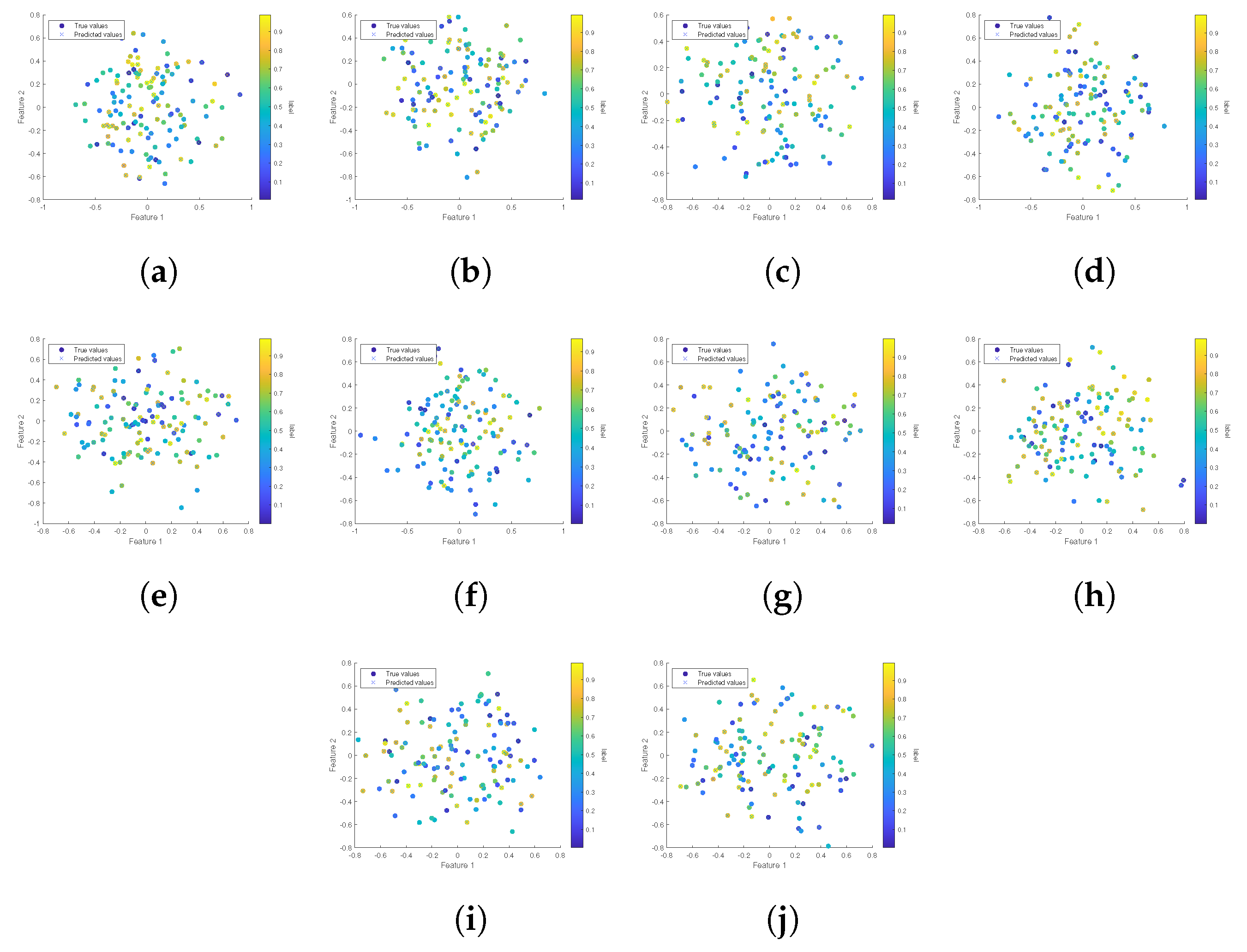
Data generation was conducted in accordance with Example 1. Principal component analysis was then employed to illustrate the distribution of the ensuing data. In this case, the five-dimensional feature data were condensed into a two-dimensional plane, with a color bar employed to signify the continuum of label values, thereby delineating the different random distributions within the interval that each original sample encountered at the data nodes.
In Figure 1a–j, the first principal component resulting from the dimensionality reduction via principal component analysis is represented along the x axis, while the second principal component is plotted along the y axis. Figure 1 suggests that the data are variably randomly distributed across the ten nodes.
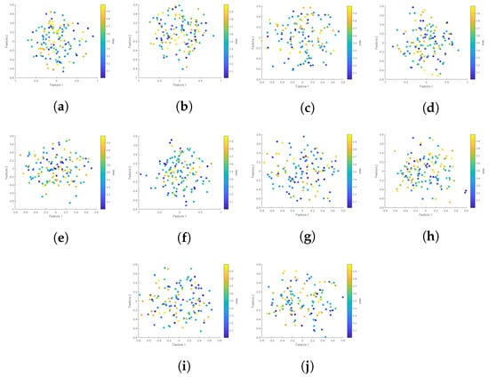
Figure 1.
Scatter plots of raw data.
Upon employing Algorithm 2 for the case illustrated in Example 1 and stipulating the number of communication rounds as 20, a two-stage process was adopted. To initiate the process, the number of data points for a single node is set to , and m, denoting the number of nodes, is varied. This produces the graphical output depicted on the left. Subsequently, with a constant node count of , the quantity of sample points per node is varied, resulting in the representation displayed on the right.
Figure 2 presents the variation in average node loss for different data quantities. Figure 2a depicts a scenario with a single-node data sample of and a node count m ranging within }. As evidenced in Figure 2a, the average loss function for nodes under Algorithm 2 descends most rapidly for and most sluggishly for . Consequently, it can be inferred that an increase in the number of nodes accelerates the decrease in the loss function, implying higher accuracy. Figure 2b considers five scenarios where and n varies within the range of . The average node loss function under Algorithm 2 is found to descend most swiftly for and most slowly for . This indicates that a reduction in the number of nodes expedites the descent of the loss function.
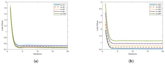
Figure 2.
Loss function plots for (a) and (b).
In addressing Example 1, Algorithm 2 was employed to determine parameters, which were then integrated into the linear model. Subsequently, the original feature data were incorporated, and labels for the original feature data were computed, which were then compared with the original data labels. Dimensionality reduction was achieved via principal component analysis to display a comparative graph of the original and model-predicted data.
Figure 3a–j employ distinct symbols to represent raw and predicted data, with color gradients depicting the corresponding label values. Dot markers indicate the sample data points post dimensionality reduction of the original data via principal component analysis. Cross markers denote data processed through the linear regression model generated by Algorithm 2, with the subsequent predicted labels presented in reduced dimensionality, also by principal component analysis. A comparison between the original and predicted data, as showcased in Figure 3, reveals a high level of accuracy attained by the linear regression model in conjunction with Algorithm 2.
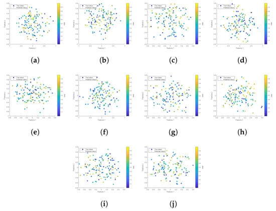
Figure 3.
Scatter plots illustrating the data from the ten nodes of Example 1 following dimensionality reduction via principal component analysis.
A comparison is also made with conventional Distributed Machine Learning (DML) [34] and Federated Learning (FL) [28]. The loss function progression of these three algorithms is depicted accordingly.
Figure 4 displays the three corresponding loss function curves. From top to bottom, the curves represent the following distinct models. The first pertains to conventional FL, the second to DML, and the third to Algorithm 2. It is observed that the loss function value for Algorithm 2 (Fed-RSADMM) decreases more rapidly than that for DML and FL and also yields the smallest value upon convergence. Figure 4 suggests that Algorithm 2 exhibits superior accuracy and faster convergence compared to traditional algorithms.
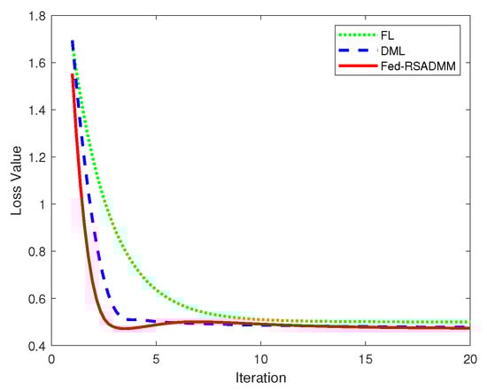
Figure 4.
Images illustrating the comparative analysis of loss functions for FL, DML, and Fed-RSADMM.
To compare the time efficiency of the algorithms, we conducted a comparative analysis of their execution times, yielding the following results.
Figure 5 provides a comparative analysis of the execution times for FL, DML, and Fed-RSADMM applied to test Example 1 over a series of iterations. The performance of the Fed-RSADMM algorithm is traced by the dashed green line, which consistently shows reduced execution times, in contrast to FL (solid blue line) and DML (dash–dot red line). The flatter trajectory of the Fed-RSADMM line across the iteration spectrum underscores its time-efficiency advantage. In essence, the results from test Example 1 endorse the Fed-RSADMM algorithm’s superior time efficiency, with its modest increase in execution time demonstrating potential for scalable and efficient processing in iterative tasks.
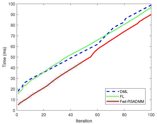
Figure 5.
Comparative execution time analysis of three algorithms for Example 1 across iterative evaluations.
Subsequently, Algorithm 3 is subjected to verification via its application to Example 2. To commence, is established within Algorithm 3, followed by a comparison with the conventional federated learning algorithm, resulting in the accompanying comparative results.
As depicted in Figure 6, the upper curve corresponds to the loss function for the traditional FL algorithm, whereas the lower curve represents Algorithm 3 (FedAvg-RSADMM). The graph illustrates that Algorithm 3 exhibits a more rapid rate of descent than the FL algorithm, indicating its superior performance over the conventional FL algorithm.
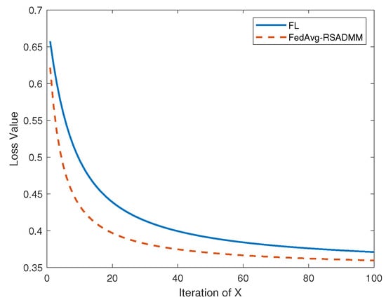
Figure 6.
Loss function comparison between FL and FedAvg-RSADMM with a setting of for the latter.
The subsequent analysis focuses on discerning the effect of on the performance of Algorithm 3. While resolving the logistic regression problem of Example 2 using Algorithm 3, the sample data size of a single node is kept constant at 1000 and 2000, while varies within the range of , leading to the ensuing comparison.
Figure 7 plots the number of iterations of the local variable (x) on the x axis against the average loss of the nodes on the y axis for different m, n, and values. As per the flow of Algorithm 3, a larger implies fewer global updates. Consequently, Figure 7 reveals a slower descent of the node’s loss function with larger values, which is attributable to the reduced number of steps in the global update, thereby conserving computational and communication resources. However, it is noted that Algorithm 3 exhibits convergence similar to that achieved with various values. This suggests that an increased effectively reduces communication and computational resource consumption, inducing only a minor error loss. Accordingly, a modest increase in in Algorithm 3 can boost its computational efficiency. The data sample size for a single node is then elevated as based on the experiment illustrated in Figure 7a for n = 1000, yielding the results portrayed in Figure 7b, which mirroring those presented in the left figure. Thus, it follows that the accuracy of Algorithm 3 remains unimpacted by the escalation of local sample data size, rendering the algorithm suitable for federated learning problems involving extensive data volumes and multiple nodes.
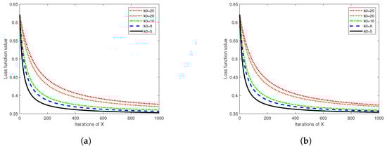
Figure 7.
Comparison of loss functions for , and (As shown in (a)), as well as for , and (As shown in (b)).
In Figure 8, the number of iterations of the global variable y is denoted by the x-axis, while the average loss of the nodes forms the y-axis, resulting in the displayed loss curve. The figure exhibits faster node loss function decreases with larger , attributable to increased local updates for sizeable during global variable updating. Consequently, fewer global update steps are required for convergence, thus significantly diminishing the number of communications and global update steps. Therefore, Algorithm 3 can be deemed effective in reducing communication losses. Again, the data sample size for a single node is amplified to based on the experiments of Figure 8a, culminating the results in Figure 8b. These demonstrate that Algorithm 3 is fitting for distributed optimization problems involving considerable local node data.
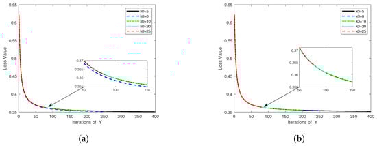
Figure 8.
Comparisons of loss functions for , and (a) and , and (b).
To investigate the impact of varying initial iteration counts () and the number of client nodes (m) on the temporal efficiency of the algorithm, we conducted a series of experiments. The parameter influences the number of local updates (), while m corresponds to the number of client nodes involved in the computation. Our objective was to ascertain whether an increased number of nodes affects the algorithm’s parallelism. The experimental outcomes are listed in Figure 9.
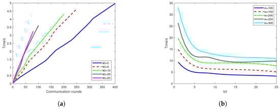
Figure 9.
(a) The relationship between iterative time and communication rounds at different values of for Algorithm 3. (b) The relationship between iterative time and with different values of m for Algorithm 3.
Figure 9a illustrates the relationship between the iterative time and the communication rounds at different values for Algorithm 3 . An increment in corresponds to a decrease in the total number of iterations required, allowing Algorithm 3 to halt earlier and utilize less iterative time. Each line in the graph represents the algorithm’s performance with a different value, demonstrating that higher values lead to quicker convergence, as evidenced by the curves leveling off sooner. This suggests that optimizing the parameter can enhance the algorithm’s efficiency, reducing computational time while maintaining convergence integrity.
Figure 9b demonstrates the relationship between the iterative time and with different numbers of nodes (m) for Algorithm 3. It is observed that an increase in m leads to a longer iteration time. However, the overall time decreases with an increase in , indicating that our algorithm exhibits favorable parallelism. Despite this, the influence of node count on computation time is not entirely negated; therefore, the potential time cost due to an increase in nodes must be considered in computational evaluations. This underscores the necessity of balancing the number of nodes against the performance gains achieved through parallel processing when deploying the algorithm in distributed computing environments.
Obviously, Algorithm 3 considers the communication and computation costs in relation to . Specifically, the framework states that the global update occurs only at certain steps (e.g., at step km being a multiple of a pre-defined integer ()). It is shown that the larger the , the less time for our algorithm to converge (see Figure 7, Figure 8 and Figure 9). In addition, the local computational complexity at each node is , where k is the iteration time. By adjusting , we can optimize the trade-off between communication efficiency and computational load, demonstrating the scalability and adaptability of the algorithm for federated learning.
5. Conclusions
This study introduces two symmetric ADMM-based federated learning algorithms relaxed steps. Algorithm 2 bolsters computational efficiency in federated learning, while Algorithm 3 capitalizes on Algorithm 2 to further optimize communication efficiency. Relevant numerical experiments were set up to illustrate the feasibility and efficiency of the algorithms. In conclusion, the two proposed algorithms exhibit rapid convergence and excellent performance. While experiments based on linear and logistic regressions were conducted on small scales and only serve as proofs of concept, in contrast to [41,42], which researched large-scale cases and realistic usage. Therefore, exploring applications related to large-scale optimization problems will be the subject of further research in the future.
Author Contributions
J.L.: data curation, theoretical derivation, methodology, software, writing—original draft preparation, and modification; Y.D.: conceptualization, formal analysis, writing—review and editing, supervision, and validation. Y.Z.: data curation, methodology, software, writing—original draft preparation, and modification. All authors have read and agreed to the published version of the manuscript.
Funding
This work was supported by the National Natural Science Foundation of China under grants 71901145 and 12371308.
Data Availability Statement
The dataset used in this paper was generated by computer simulations to support the experimental data.
Acknowledgments
We acknowledge the efforts of the editorial board and anonymous reviewers for their thorough evaluation of our manuscript. Their comments and recommendations contributed to the refinement of our research paper.
Conflicts of Interest
No conflicts of interest exist with respect to the submission of this manuscript, and the manuscript was approved by all authors for publication. We would like to declare that the work described is original research that has not been published previously and is not under consideration for publication elsewhere, either in whole or in part. All listed authors approved of the manuscript that is enclosed. The authors declare that they have no known competing financial interests or personal relationships that could appeared to have influenced the work reported in this paper.
Appendix A
Appendix A.1. Proof of Lemma 3
For notational simplicity, hereafter, we denote
According to Definition (4), we provide the optimality conditions for the subproblems in Fed-RSADMM,
Based on the update steps for and , we have
The optimality conditions for the subproblems involving , y, and are obtained as follows:
Considering the updating methodology for u, it can be inferred that
Regarding the subproblem of ,
Hence,
Therefore,
According to the subproblem of y,
Therefore, it follows that
After simplification, it is obtained as:
In summary, it is evident that
By incorporating the subproblem of , we consider the following formulation:
The result is given by
Integrating the subproblem of y, now, we consider the following formulation:
The outcome is expressed as follows:
Utilizing the updating step of the multiplier (), in conjunction with Equation (A5), it is found that
By cumulatively considering (A13), (A15), and (A16) with , it is concluded that
Upon further integration of , the Lipschitz continuity of and the Cauchy–Buniakowsky–Schwarz inequality yield
Let , , and it follows that
wherein
Appendix A.2. Proof of Lemma 4
Given that the sequence of is bounded, it can be deduced that the sequence has a limit point. Without loss of generality, we assume that is a limit point of the sequence of , and the subsequence of converges to . Since is lower semi-continuous, is also lower semi-continuous. Hence,
The above equation shows that has a lower bound. It also follows from Lemma 3 that is monotonically decreasing such that is also monotonically decreasing, so there is convergence. The sequence of has monotonically convergent subsequences such that its whole column converges and has
Shifting the term for (35) results in
Taking the sum over the finite terms of the above inequality and the limit yields
Consequently, . Further integration with , from Equation (A5) shows that
therefore,
Then, according to the Cauchy inequality, we obtain
This integrates with . It holds that . Therefore, it can be immediately established that
The proof is complete.
Appendix A.3. Proof of Theorem 1
(1) From the definition of , conclusion (I) is validated.
(2) If , there exists a subsequence (, ) such that . Additionally, from Lemma 4, we know ; thus, . Also, since is the solution to the x subproblem in Algorithm 2, for any , it holds that
Subsequently,
According to this, together with the lower semi-continuity of and given , then
. Therefore, . Therefore, due to the closedness of , considering in Equation (23) and taking the limit as yields
This, in conjunction with Definition 3, establishes that .Q.E.D.
Appendix A.4. Proof of Lemma 5
First, based on Equations (23)–(25), the definition of , and the non-expansive nature of the proximity operator, it can be shown that
Additionally, from (23), it is known that
Next, integrating (24) and (25), it is established that
Finally, according to Equations (A23)–(A25), there exist positive numbers () such that
Appendix A.5. Proof of Theorem 2
(1) As for Lemma 4, . This, in conjunction with (37), yields . Furthermore, as is monotonically decreasing, . Furthermore, integrating with Assumption 2, there exists and a positive integer () such that
Consequently, conclusion (1) is validated. (2) Setting , it follows that
Combined with the above conclusion (1), . Utilizing the triangle inequality, it is further deduced that
According to Assumption 3, for any , it holds that ; therefore, we have . Therefore, according to (A29), there exists a positive integer () and a constant () such that .
Next, we analyze the properties of . According to Theorem 1 (2), it follows that any accumulation point of is a stable point of . It is also proved by Theorem 1(2) that . Considering that converges, . Hence, remains constant for the set of accumulation points.
Since , . Consequently, integration with Assumption 3 yields
(3) According to (A28), it is understood that
From the definition of ALF in (16), it is deduced that
On the other hand, due to the convexity of , it is inferred that
Combining the above two equations with (A5) and (A32) and simplifying (A33), we obtain
Furthermore, according to simple calculations and by integrating (A31), there must exist positive numbers () such that
Furthermore, based on the aforementioned conclusion (2), Assumption 2, and Lemma 5, it is found that
where . This, together with Equation (35), the inequality, and the condition yield
Hence, for sufficiently large values of k, it holds that
Consequently, the sequence is Q-linearly convergent.
Appendix A.6. Proof of Theorem 3
According to Equation (35), it can be established that
From Theorem 2, we know that the sequence of is Q-linearly convergent, and there exist and such that This, in combination with Equation (36), implies the existence of and such that
Hence, it can be concluded that
where . Therefore, for any , it holds that
This indicates that is a Cauchy sequence; hence, it converges. Let its limit point be denoted as ; then,
Furthermore, from Theorem 1(1), it is understood that the sequence of converges to the steady point of at the rate of R-linear convergence.
References
- McMahan, B.; Moore, E.; Ramage, D.; Hampson, S.; Arcas, B.A.y. Communication-efficient learning of deep networks from decentralized data. In Proceedings of the 20th International Conference on Artificial Intelligence and Statistics, PMLR, Fort Lauderdale, FL, USA, 20–22 April 2017; pp. 1273–1282. [Google Scholar]
- Li, T.; Sahu, A.K.; Zaheer, M.; Sanjabi, M.; Talwalkar, A.; Smith, V. Federated optimization in heterogeneous networks. Proc. Mach. Learn. Syst. 2020, 2, 429–450. [Google Scholar]
- Zhang, X.; Hong, M.; Dhople, S.; Yin, W.; Liu, Y. Fedpd: A federated learning framework with adaptivity to non-iid data. IEEE Trans. Signal Process. 2021, 69, 6055–6070. [Google Scholar] [CrossRef]
- Yang, Q.; Liu, Y.; Chen, T.; Tong, Y. Federated machine learning: Concept and applications. Acm Trans. Intell. Syst. Technol. (TIST) 2019, 10, 1–19. [Google Scholar] [CrossRef]
- Liu, T.; Wang, Z.; He, H.; Shi, W.; Lin, L.; An, R.; Li, C. Efficient and secure federated learning for financial applications. Appl. Sci. 2023, 13, 5877. [Google Scholar] [CrossRef]
- Zeng, Q.; Lv, Z.; Li, C.; Shi, Y.; Lin, Z.; Liu, C.; Song, G. FedProLs: Federated learning for IoT perception data prediction. Appl. Intell. 2023, 53, 3563–3575. [Google Scholar] [CrossRef]
- Manias, D.M.; Shami, A. Making a case for federated learning in the internet of vehicles and intelligent transportation systems. IEEE Netw. 2021, 35, 88–94. [Google Scholar] [CrossRef]
- Posner, J.; Tseng, L.; Aloqaily, M.; Jararweh, Y. Federated learning in vehicular networks: Opportunities and solutions. IEEE Netw. 2021, 35, 152–159. [Google Scholar] [CrossRef]
- Konečný, J.; McMahan, B.; Ramage, D. Federated optimization: Distributed optimization beyond the datacenter. arXiv 2015, arXiv:1511.03575. [Google Scholar]
- Satish, S.; Nadella, G.S.; Meduri, K.; Gonaygunta, H. Collaborative Machine Learning without Centralized Training Data for Federated Learning. Int. Mach. Learn. J. Comput. Eng. 2022, 5, 1–14. [Google Scholar]
- Zhou, S.; Li, G.Y. Federated learning via inexact ADMM. IEEE Trans. Pattern Anal. Mach. Intell. 2023, 45, 9699–9708. [Google Scholar] [CrossRef]
- Elgabli, A.; Park, J.; Ahmed, S.; Bennis, M. L-FGADMM: Layer-wise federated group ADMM for communication efficient decentralized deep learning. In Proceedings of the 2020 IEEE Wireless Communications and Networking Conference (WCNC), Seoul, Republic of Korea, 25–28 May 2020; IEEE: Piscataway, NJ, USA, 2020; pp. 1–6. [Google Scholar]
- Zhang, X.; Khalili, M.M.; Liu, M. Improving the privacy and accuracy of ADMM-based distributed algorithms. In Proceedings of the International Conference on Machine Learning, PMLR, Stockholm, Sweden, 10–15 July 2018; pp. 5796–5805. [Google Scholar]
- Guo, Y.; Gong, Y. Practical collaborative learning for crowdsensing in the internet of things with differential privacy. In Proceedings of the 2018 IEEE Conference on Communications and Network Security (CNS), Beijing, China, 30 May–1 June 2018; IEEE: Piscataway, NJ, USA, 2018; pp. 1–9. [Google Scholar]
- Zhang, X.; Khalili, M.M.; Liu, M. Recycled ADMM: Improve privacy and accuracy with less computation in distributed algorithms. In Proceedings of the 2018 56th Annual Allerton Conference on Communication, Control, and Computing (Allerton), Monticello, IL, USA, 2–5 October 2018; IEEE: Piscataway, NJ, USA, 2018; pp. 959–965. [Google Scholar]
- Huang, Z.; Hu, R.; Guo, Y.; Chan-Tin, E.; Gong, Y. DP-ADMM: ADMM-based distributed learning with differential privacy. IEEE Trans. Inf. Forensics Secur. 2019, 15, 1002–1012. [Google Scholar] [CrossRef]
- He, S.; Zheng, J.; Feng, M.; Chen, Y. Communication-efficient federated learning with adaptive consensus admm. Appl. Sci. 2023, 13, 5270. [Google Scholar] [CrossRef]
- Ding, J.; Errapotu, S.M.; Zhang, H.; Gong, Y.; Pan, M. Stochastic ADMM based distributed machine learning with differential privacy. In Proceedings of the Security and Privacy in Communication Networks: 15th EAI International Conference, SecureComm 2019, Orlando, FL, USA, 23–25 October 2019; Proceedings, Part I 15. Springer International Publishing: Berlin/Heidelberg, Germany, 2019; pp. 257–277. [Google Scholar]
- Hager, W.W.; Zhang, H. Convergence rates for an inexact ADMM applied to separable convex optimization. Comput. Optim. Appl. 2020, 77, 729–754. [Google Scholar] [CrossRef]
- Yue, S.; Ren, J.; Xin, J.; Lin, S.; Zhang, J. Inexact-ADMM based federated meta-learning for fast and continual edge learning. In Proceedings of the Twenty-Second International Symposium on Theory, Algorithmic Foundations, and Protocol Design for Mobile Networks and Mobile Computing, Shanghai, China, 26–29 July 2021; pp. 91–100. [Google Scholar]
- Ryu, M.; Kim, K. Differentially private federated learning via inexact ADMM with multiple local updates. arXiv 2022, arXiv:2202.09409. [Google Scholar]
- Zhang, S.; Choromanska, A.E.; LeCun, Y. Deep learning with elastic averaging SGD. In Proceedings of the Advances in Neural Information Processing Systems 28, Montreal, QC, Canada, 7–12 December 2015. [Google Scholar]
- Koloskova, A.; Stich, S.U.; Jaggi, M. Sharper convergence guarantees for asynchronous SGD for distributed and federated learning. In Proceedings of the Advances in Neural Information Processing Systems 35, New Orleans, LA, USA, 28 November–9 December2022; pp. 17202–17215. [Google Scholar]
- Yu, H.; Yang, S.; Zhu, S. Parallel restarted SGD with faster convergence and less communication: Demystifying why model averaging works for deep learning. In Proceedings of the AAAI Conference on Artificial Intelligence, Honolulu, HI, USA, 27 January 27–1 February 2019; Volume 33, pp. 5693–5700. [Google Scholar]
- Dai, S.; Meng, F. Addressing modern and practical challenges in machine learning: A survey of online federated and transfer learning. Appl. Intell. 2023, 53, 11045–11072. [Google Scholar] [CrossRef]
- Wang, J.; Joshi, G. Cooperative SGD: A unified framework for the design and analysis of local-update SGD algorithms. J. Mach. Learn. Res. 2021, 22, 1–50. [Google Scholar]
- Smith, V.; Forte, S.; Ma, C.; Takac, M.; Jordan, M.I.; Jaggi, M. CoCoA: A general framework for communication-efficient distributed optimization. J. Mach. Learn. Res. 2018, 18, 1–49. [Google Scholar]
- Konečný, J.; McMahan, H.B.; Ramage, D.; Richtárik, P. Federated optimization: Distributed machine learning for on-device intelligence. arXiv 2016, arXiv:1610.02527. [Google Scholar]
- Konečný, J.; McMahan, H.B.; Yu, F.X.; Richtárik, P.; Suresh, A.T.; Bacon, D. Federated learning: Strategies for improving communication efficiency. arXiv 2016, arXiv:1610.05492. [Google Scholar]
- Li, T.; Sahu, A.K.; Sanjabi, M.; Zaheer, M.; Talwalkar, A.; Smith, V. On the convergence of federated optimization in heterogeneous networks. arXiv 2018, arXiv:1812.06127. [Google Scholar]
- Rockafellar, R.T.; Wets RJ, B. Variational Analysis; Springer Science & Business Media: Berlin/Heidelberg, Germany, 2009. [Google Scholar]
- Parikh, N.; Boyd, S. Proximal algorithms. Found. Trends® Optim. 2014, 1, 127–239. [Google Scholar] [CrossRef]
- Shalev-Shwartz, S.; Ben-David, S. Understanding Machine Learning: From Theory to Algorithms; Cambridge University Press: Cambridge, UK, 2014. [Google Scholar]
- LeCun, Y.; Bengio, Y.; Hinton, G. Deep learning. Nature 2015, 521, 436–444. [Google Scholar] [CrossRef] [PubMed]
- Bottou, L. Large-scale machine learning with stochastic gradient descent. In Proceedings of the COMPSTAT’2010: 19th International Conference on Computational Statistics, Paris, France, 22–27 August 2010; Keynote, Invited and Contributed Papers. Physica-Verlag HD: Heidelberg, Germany, 2010; pp. 177–186. [Google Scholar]
- Wang, S.; Tuor, T.; Salonidis, T.; Leung, K.K.; Makaya, C.; He, T.; Chan, K. Adaptive federated learning in resource constrained edge computing systems. IEEE J. Sel. Areas Commun. 2019, 37, 1205–1221. [Google Scholar] [CrossRef]
- Zhu, Y. An augmented ADMM algorithm with application to the generalized lasso problem. J. Comput. Graph. Stat. 2017, 26, 195–204. [Google Scholar] [CrossRef]
- Yang, K.; Jiang, T.; Shi, Y.; Ding, Z. Federated learning via over-the-air computation. IEEE Trans. Wirel. Commun. 2020, 19, 2022–2035. [Google Scholar] [CrossRef]
- Jia, Z.; Gao, X.; Cai, X.; Han, D. Local linear convergence of the alternating direction method of multipliers for nonconvex separable optimization problems. J. Optim. Theory Appl. 2021, 188, 1–25. [Google Scholar] [CrossRef]
- Jia, Z.; Gao, X.; Cai, X.; Han, D. The convergence rate analysis of the symmetric ADMM for the nonconvex separable optimization problems. J. Ind. Manag. Optim. 2021, 17, 1943–1971. [Google Scholar] [CrossRef]
- Kadu, A.; Kumar, R. Decentralized full-waveform inversion. In Proceedings of the 80th EAGE Conference and Exhibition 2018, Copenhagen, Denmark, 11–14 June 2018; European Association of 1Geoscientists and Engineers: Utrecht, The Netherlands, 2018; Volume 2018, pp. 1–5. [Google Scholar]
- Yin, Z.; Orozco, R.; Herrmann, F.J. WISER: Multimodal variational inference for full-waveform inversion without dimensionality reduction. arXiv 2024, arXiv:2405.10327. [Google Scholar]


Disclaimer/Publisher’s Note: The statements, opinions and data contained in all publications are solely those of the individual author(s) and contributor(s) and not of MDPI and/or the editor(s). MDPI and/or the editor(s) disclaim responsibility for any injury to people or property resulting from any ideas, methods, instructions or products referred to in the content. |
© 2024 by the authors. Licensee MDPI, Basel, Switzerland. This article is an open access article distributed under the terms and conditions of the Creative Commons Attribution (CC BY) license (https://creativecommons.org/licenses/by/4.0/).