Abstract
In this paper, we first prove the existence and uniqueness of the solution to a variable-order Caputo–Fabrizio fractional stochastic differential equation driven by a multiplicative white noise, which describes random phenomena with non-local effects and non-singular kernels. The Euler–Maruyama scheme is extended to develop the Euler–Maruyama method, and the strong convergence of the proposed method is demonstrated. The main difference between our work and the existing literature is the fact that our assumptions on the nonlinear external forces are those of one-sided Lipschitz conditions on both the drift and the nonlinear intensity of the noise as well as the proofs of the higher integrability of the solution and the approximating sequence. Finally, to validate the numerical approach, current results from the numerical implementation are presented to test the efficiency of the scheme used in order to substantiate the theoretical analysis.
Keywords:
variable-order Caputo–Fabrizio fractional stochastic differential equation; non-singular non-local effect; Euler–Maruyama method; strong convergence MSC:
34A08; 35R11; 39A50; 60H10; 60H15; 60H30; 60H35; 65C30
1. Introduction
Mathematical models of natural and physical phenomena have always played a central and critical role in science since the times of Newton and Euler. The fractional derivatives have been crucial in applied mathematics and mathematical sciences since the time of Leibniz. Note that the foundation of fractional derivatives was pioneered by Liouville. These fractional systems are often of evolutionary type, time-dependent, linear or nonlinear cases; within their range of important applications we find aircraft simulation, fractional Newtonian fluids, flow through porous media, weather prediction, image restoration, image processing, and inverse image processing, just to name a few. Among others, these fractional systems can be used to describe behaviors of the most fascinating and challenging issues in the mathematical community. Despite much progress, the field is still open, and it is often quiet challenging to obtain regular and global solutions to the fractional Navier–Stokes and hydrodynamics models of turbulence for just the case of a deterministic setting. For the fractional stochastic counterparts, it is even much more harder in certain cases, for example, the existence of invariant measure in any dimension.
Over the last few decades, stochastic fractional partial differential equations (SFPDEs) have been investigated by several authors, and many results were obtained on its theory and also applied to various real world phenomena. We refer, for example, to [1,2,3,4,5,6]. The analysis of systems with a Caputo derivative of variable order without a singular kernel presents a cutting edge and a mathematical framework for modeling complex systems influenced by both randomness and non-local interactions. Instead of approaches to calculus, these equations make use of the adaptable nature of variable-order Caputo derivatives, which adjust to varying conditions and capture subtle memory effects. By incorporating stochastic terms to accommodate randomness in system dynamics often represented by Wiener or Gaussian processes, SFPDEs with variable-order Caputo derivatives provide a tool for analyzing intricate phenomena across various fields, such as some branches of physics (nematic liquid crystal), mechanics (stochastic electro-rheological fluids), and climate, atmospheric, ocean dynamics (shallow water systems), turbulent flow in gas pipelines, and porous media problems.
The application of the Caputo derivative with variable order goes beyond standard partial differential equations, allowing for the exploration of anomalous diffusion, non-local interactions and spatio-temporal correlations in diverse systems. The lack of kernels in the variable-order Caputo derivative improves stability and enables efficient computational methods for solving SFPDEs. This progress creates opportunities to study emerging behaviors, multi-fractal patterns, and complex dynamics in disciplines such as physics, biology, finance, and engineering, to name just a few.
Currently, notable works from several researchers delve into the characteristics and uses of variable-order Caputo derivatives in calculus. These investigations offer perspectives on the underpinnings and real world significance of utilizing variable-order Caputo derivatives to model and analyze intricate systems influenced by stochastic fractional partial differential equations. In this direction, several authors extended many results in order to incorporate the definition of the Caputo derivative to model useful problems and also complex phenomena either through the temporal variable or via a spacial component or as space–time fractional derivatives. For instance, we refer to a more recent manuscript in this direction; see [7] and the references therein for attenuation of the Caputo–Djrbashian fractional time derivative in modeling some inverse problems for wave equations. For the solution of stochastic evolution equation using the Marchaud fractional derivative, we refer to the work in Zhou et al. [8], and more recent results in this direction can be obtained in [9,10,11,12,13,14] and the references therein. For the exact solution using the conformable derivative, we refer to papers [12] and Abu-Shady and Mohammed in [15,16,17], and further extension can be found in the references [18,19,20,21]. For the the Wick-type fractional derivative, we refer to, for instance, the manuscript 0f Kim H. et al. [22]. For the fractional PDEs and their numerical solutions, we refer to, e.g., the work in [23,24], where further references can also obtained. For the random attractor in the fractional sense, see, for example, the manuscript [25]. For the fraction derivatives in the sense of Jumarie’s modified Riemann–Liouvile type, we refer the reader to [26], where further references are given therein. Most recent results concerning the various extensions of the Riemann–Liouville fractional derivatives can be found in the work of Jacky and Anna in [27].
Stochastic processes in many fields and applications can be described by classical stochastic differential equations (SDEs) of the form
Let us mention a few, such as engineering, finance, and physics, because fractional stochastic differential equations are becoming a powerful tool in modeling problems in many disciplines. Many stochastic processes can be described (or modeled) by the system given in (1), for instance, a particle in the viscoelastic medium has random-movement Brownian motion with its resistance of a memory effect that leads to a fractional stochastic differential equation (FSDE); see [28,29,30,31,32,33] for more details. Despite knowing that multiple time-scale processes are not easy to model by using FSDE, however, we can emphasize the modeling of the accuracy of numerical approximation of non-physical initial weak singularity problems through FSDE; see instance, [24,34] where further references can be found therein. Henceforth, it is clearly challenging to obtain the probabilistic strong solutions for SFPDEs. Therefore, various numerical approximations of the solutions to both the deterministic FPDEs and SFPDEs have been proposed to deal with the issues of strong convergence and error estimates based on the Euler–Maruyama approximating techniques. See, for instance, the examples of a range of numerical approximations in the recent results in [32,35,36,37,38,39,40,41,42,43,44]. For the convergence of relative entropy for the Euler–Maruyama approximation, we refer to the most recent work of Yu in [43]; the split-step truncated EM approach was observed in [45]. Further exposition can be found in [46,47].
For the first time, Zhiwei et al. [33] analyzed, discretized, and obtained a solution of a two-time-scale variable-order time-FSDE using the Riemann–Liouville fractional differential operator with the non-Lipschitz weakly singular kernel. Similarly, Hong et al. [48] obtained the solution of the variable-order time-fractional diffusion equations and a variable-order FSDE of two-time scales with a Riemann–Liouville fractional differential operator presented by Xiangcheng et al. [49]. More detailed exposition about the Caputo derivatives can be found in [50] in this direction. For more engineering applications, we refer to [51]. On the other hand, for the solvability of time-fractional diffusion equations of constant order, we refer to Martin [24]. However, all the above papers dealt with the numerical approximations of FSPDEs with kernels. Therefore, the asymptotic and ergodic environment of the type of probabilistic solutions in this work have not yet been studied in the literature. Thus, so far, the asymptotic behavior of the underlying problem can still be treated as an open problem.
To the best of our knowledge, the strong convergence of the EM scheme for the nonlinear fractional stochastic differential equations without singular kernels has not yet been investigated in the existing literature. Having said that, therefore, the present work is the first one to consider proving the existence and uniqueness of a probabilistic strong solution to fractional stochastic differential equations with non-singular kernels subjected to nonlinear perturbation. Hence, this motivates us to state and prove a range of results on a priori estimates, error estimates, and the strong convergence of the EM approximation method for the problem under consideration. In fact, the underlying problem describes the more complex random phenomena with non-local effect. In addition, we develop and prove the strong convergence of the Euler-type scheme. Finally, as a matter of fact, we present our numerical experiments in order to substantiate the analysis of the problem under consideration. The current results from the numerical experiments are then compared with the results in the existing literature using both MATLAB and Python programmings. The main difference between the results carried out in this paper and those in [33] is highlighted by the existence and uniqueness carried out not only without the Lipschitz conditions as used in [33] but also the fact that we do not use the kernel, as in [33]. Instead of adapting the Riemann–Liouville fractional differential operator, as in [33], we use the new Caputo fractional derivative with variable order and study numerical solutions of FSDE without a singular kernel.
In this paper we consider the new Caputo–Fabrizio fractional derivative with variable order and study numerical solutions of FSDE without a singular kernel in the form
where f and b are nonlinear external terms representing the drift and the intensity of the noise, respectively. Here, W is a Wiener process and is the new Caputo–Fabrizio fractional derivative of order ; see the subsection below for more details and properties of this operator. Note the assumptions on both function f and b will be subsequently specified.
1.1. Important Properties of
We recall from [50] that the Caputo fractional derivative of order is defined by
where , , and for and . Here, is the kernel, defined as
We can list some of the properties and drawbacks of this operator in the remark below.
Remark 1.
Note that, for , the kernel in the above definition becomes singular, that is, . This singularity is disadvantageous in modeling real-world phenomena. This fact can reduce the application of this operator to more complex problems. Furthermore, we also note in the definition of the operator , the presence of the function , meaning that the derivative of u must exist in the ordinary sense before we can define or compute any expression with the above defined operator.
Now set
and change the constant by in the definition of the operator . Then, according to [52], the new Caputo–Fabrizio derivative of order , can be defined as FD without a singular kernel as follows (after normalizing):
Remark 2.
At first glance, we notice that, for , the new kernel . In contrast to , the new kernel is not singular and it is, in addition, very much a regular kernel. Moreover, as for the operator , we also observe that requires the function u to admit a first derivative in the ordinary sense. However, this can be addressed below.
Arguing similarly as in [50], one can easily define the operator for function and by setting
where is a normalized constant depending on .
From this definition, we remark that the system modeled by the operator can describe non-local systems, which are able to model fluctuations that cannot be captured by the usual operator .
1.2. Motivational Background
Exploring systems that display unpredictability and distant connections is fundamental in contemporary science and engineering practices. The mathematical representation of these systems frequently necessitates instruments that surpass traditional calculus by integrating components capable of managing both randomness and memory impacts. Fractional stochastic partial differential equations have recently been among the most popular areas in describing and understanding mathematically complex behaviors of robust systems such as the Navier–Stokes and hydrodynamics models of turbulence fluids. It is worth mentioning that the presence of stochastic forces in a model (fractional type) can lead to new phenomena that are very difficult to describe using their deterministic fractional counterparts. The generalization of Navier–Stokes equations by fractional Navier–Stokes systems can be used to better describe and analyze in practice the compressible and incompressible fluids dynamics. Due to the challenging task in computing and analyzing the behavior of some complex phenomena, several researchers have recently proposed different classes of models. Among those models, we mention the shell fractional system that consists of infinitely many differential equations that can be used to model behaviors similar to the fractional Navier–Stokes, and many other similar properties of the classical Navier–Stokes can be studied. Moreover, other things that can be explored are the attempt at relaxing some assumptions and homogeneity, studying boundary conditions and boundary layers, and treating other physical phenomena.
Utilizing adaptable derivatives in these equations allows for a more accurate representation of real-world events that helps capture nuances that are often missed by the conventional models.
The enhanced capabilities of the order Caputo derivative without singular kernels represent a major step forward in fractional calculus by enhancing stability and effectiveness in computational techniques across various industries, like physics with prevalent anomalous diffusion phenomena; biology with intricate spatio-temporal patterns; and finance, with market dynamics displaying fractal characteristics. By removing kernels from the models structure, it not only enhances its resilience but also makes it more viable computationally, thus paving the way for exploring fresh avenues in simulating and comprehending systems that are impacted by both deterministic and stochastic elements.
Innovations in the field have revealed that SFPDEs incorporating Caputo derivatives of varying orders offer perspectives on complex system behaviors that conventional models find challenging to explain fully. For example, intricate phenomena characterized by scale processes, non-local interactions, and intricate random dynamics present in viscoelastic materials or financial markets stand to benefit from this method. These progressions not only enrich our theoretical comprehension but also hold practical significance in refining algorithms and enhancing numerical techniques applied in simulations across diverse scientific domains.
The task within this manuscript is to initiate the study of some interesting classes of nonlinear FSPDEs driven by white noise and also to investigate several results: first the issues of well-posedness (existence and uniqueness) of these systems, rate of convergence, strong convergence, a priori estimates, and higher integrability on the solutions, error estimates, and the approximate solutions.
In our research project, we are seeking to extend our knowledge in this particular field even further by investigating a novel approach not previously explored. We examine how a robust strong probabilistic solution can exist for fractional stochastic differential equations characterized by non-singular kernels and impacted by nonlinear perturbations for the very first time ever. This study opens up pathways for delving deeper into intricate stochastic systems and enhancing computational methodologies for better outcomes overall. Our findings underscore distinctions and advancements compared to current techniques in this area of study and lay down a strong groundwork that will shape future investigations in stochastic processes and fractional calculus. The discoveries have the potential to result in advancements across various sectors, such as material science and financial engineering, by addressing uncertainties and memory influences that are essential in these fields.
To the best of our knowledge, the strong convergence of the EM scheme for nonlinear fractional stochastic differential equations without singular kernels has not yet been studied in the corresponding literature. Therefore, this work is the first one to consider proving the existence and uniqueness of a probabilistic strong solution to the fractional stochastic differential equations with non-singular kernel subjected to nonlinear white noise. Hence, this clearly motivates us to establish new results on a priori bounds, higher integrability, error estimates, and the strong convergence of the EM approximation method for the problem under consideration.
1.3. Organization of the Paper
The remaining sections of this paper are structured as follows. In Section 2, we prove that the convergence of the Euler–Maruyama approximation and the associated numerical solution has a bounded pth moment for a some . In Section 3, we impose further assumptions on the nonlinear external forces f and g to ensure that has bounded moments. In Section 4, we focus on establishing an optimal rate of convergence of the method established in Section 3. This section is augmented to a more widely used implicit variant of Euler–Maruyama by relating the notion introduced in Section 2 of implicit methods with the result obtained in Section 4. In Section 5, we draw concluding remarks. The major tools are listed in Appendix A.
2. Convergence, Continuity, and Uniqueness of the Solution for Equation (2)
In this section, we prove the existence of numerical solutions of FSDE (2). We start by reformulating FSDE (2) similar to Yang et al. [33].
Let be a filtered probability space equipped with a filtration satisfying the usual conditions. Let W be a Wiener process defined on this probability space, associated with the filtration, and let be a random variable that is independent of the Wiener process W. We consider to be a Brownian motion with respect to the filtration
where is the natural -algebra generated by , which is a second-order variable, and is independent of Brownian motion with a history up to time t. Here and subsequently, we assume that the filtration is complete and right-continuous. Indeed, hereafter, we assume that the nonlinear external terms are continuous with respect to the first variable t and Lipschitz with respect to the second variable u. We denote the Euclidean vector norm by the symbol .
In order to obtain the existence and uniqueness of solution (strong) to the problem under consideration, we need to provide some assumptions on a the nonlinear terms, the drift f, and the diffusion coefficients b that will be needed subsequently.
Assumptions:
- (i)
- Suppose that are both one-sided Lipschitz nonlinear continuous functions and, in addition, the function b is Lipschitz nonlinear continuous function with respect to u, respectively, i.e., for , then there exists a constant depending only on R, such that ; it holds that
- (ii)
- We assume that the nonlinear term b is measurable a.e., t, and that there exists such that
- (iii)
- Let , the space of functions that are differentiable and continuous on the interval such that there is such that
To represent Equation (2) in stochastic process form, first we integrate the fractional derivative part of (2) from by applying the same technique in Xiangcheng et al. [49]. We first have
where
Our main objective is to find a stochastic process u that will satisfy the stochastic integral below. For this purpose, modulo a stopping time argument, we can insert Equation (10) in (2), with , to generate a stochastic process , which is progressively measurable on such that the following stochastic integral holds:
Our first and primary goals are to investigate the strong convergence of numerical approximation in the scenario, where f and b are both one-sided Lipschitz with b in addition being locally Lipschitz. Subsequently, denote some generic positive constants that may change from time to time throughout the paper.
In order to proceed with the proof of this result in Theorem 1, we rely on the Picard iteration approach. For this purpose, we define a general term of the Picard sequence by setting
with .
This above Picard sequence can be generated using the Picard iteration method. Therefore, we follow the arguments of the celebrated work of Etienne Pardoux in [53] to deal with the terms in the sequence. Before we delve into the proof of Theorem 1, we first introduce the following result.
Lemma 1.
Proof.
Applying Ito’s formula to the function , we have
In order to estimate every term in (16), we rely on Assumptions (3), (4), (6), and (7), the Burkholder–Davis–Gundy (BDG) inequality, Young’s inequality, and the Cauchy–Swarz inequality to deal with each term in (16). For this purpose, we deal with the integrals in (16) separately. Therefore, we take mathematical expectation of both sides of (16) then apply the supremum to both sides to obtain the corresponding relation from which we estimate the remaining terms as below. We have
Using the assumption in item (i) along with Fubini’s theorem, we infer from the Young and Cauchy inequalities that there exists a constant such that
As for the term in , we first apply the BDG inequality and then use Assumption (7) and Young’s inequality to obtain
Similarly, in the case for the bound of , we can also estimate the term using Assumption (7) to obtain
Combining all the estimates (17)–(20), we obtain
On the other hand, raising the expression in (14) to the power 2 and the taking mathematical expectation and the supremum and using Jensen’s inequality, we obtain that
Similarly as in the estimates for , we rely on the same techniques to deal with the estimates for . Therefore, we use Assumptions (3)–(8) along with the BDG, Young, Cauchy, and Jensen inequalities to obtain the corresponding relations needed for the estimates. We hence deduce the estimate for and as follows:
Due to Assumption (6) along with the Young and Cauchy inequalities, we infer that
As for the stochastic term, we use Assumption (7) and apply Burkholder–Davis–Gundy’s inequality along with the Young and Cauchy inequalities to obtain
Combining all estimates (23)–(25), we obtain
In order to carry on with the remaining parts of the proof, we define the function by setting
We remark by definition of that
from which we infer that
where Q is a constant depending only on , and .
Arguing similarly as in [33], we heavily rely on the principle of mathematical induction to estimate the function . For this purpose, we first address the case of and deal with the corresponding relation as follows:
We infer from relation (16) and BDG inequality (25) with that
where is a constant depending only on , , and T. It implies the estimate of the first term . This holds true.
For , we have
This holds true as well.
Similarly, for we have
This is true.
Now, we assume that the induction step and the inductive hypothesis both hold true; for we have that
from which we deduce that the series (32) can be written as
Here, stands for the Mittag-Leffler function and the above series duly converges. Therefore,
from which, along with Chebyshev’s inequality, we infer that
Hence, we use the Borel–Cantelli lemma to deduce that the sequence converges uniformly to the process on . □
We are now ready to proceed with the Proof of Theorem 1.
Proof.
In order to obtain the integrability in Theorem 1, we need to estimate every term in the right-hand side of (14). For this purpose, we first rely on the result of Lemma 1 and use the same sequence as defined above. We therefore notice that the difference is given by
In order to obtain the best estimates, we first apply Ito’s formula to the functions and . Second, we estimate the terms in the expression of directly without using the expressions coming from Ito’s formula and then combine the terms coming from both relations to get the best estimates required for the proof of this theorem.
For this purpose, on one hand, applying Ito’s formula to the functions and , we obtain
from which we infer that
Our next task is to separately estimate every term on the right side of Equation (35). To bound the first term of (35), we can apply Lemma A1, the Cauchy–Schwarz inequality, and Assumptions (3) to (8). We also apply the Young’s inequality modulo a stopping time to obtain
We can proceed to estimate the term . Note that, by virtue of triangle and Jensen inequalities and due to the assumption in item (i) along with Fubini’s Theorem, we have
In order to proceed with the estimate of the term , we first use the one-sided Lipschitz assumption given in item (i), secondly the BDG inequality, and thirdly Young’s inequality to assert that there exists a constant such that
Finally, by applying Ito’s isometry, Lemma A2 (Appendix A), and Assumptions (3) to (8), we can bound the third term of (35) and obtain using a stopping time argument that
where is constant depending on R only. This gives us the estimate on the last term .
Now we combine all the estimates from (35) to (39) and (35) as well as applying Young’s inequality to obtain
where .
On the other hand, we notice that
where
This indicates to us that we must also estimate every term in (41). Then, by the Jensen inequality, we have
from which we infer that
Our next task is to separately bound every term on the right side of Equation (42). To bound the first term of (42), we can apply Lemma A1, the Cauchy–Schwarz inequality, and Assumptions (3) to (8). We also apply the Young’s inequality modulo a stopping time to obtain
Next, by applying Cauchy and Young’s inequalities and Assumptions (3) to (8), we can bound the second term of (35) as follows:
Finally, by applying Ito isometry, Lemma A2, Burkhlder–Davis–Gundy, and Assumptions (3) to (8), we can bound the third term of (42) and obtain using a stopping time that
where is constant as the one given by Lemma A2. Now we combine all inequalities (36)–(45) with relation (35) and apply Young’s inequality to obtain
where .
Next, we use mathematical induction to find the estimate for the terms in relation (47). For this purpose, for , we reformulate and estimate the terms in the right-hand side of Equation (42) as follows. Set
where
Using Equation (35) with , applying the Jensen inequality, and using Assumptions (3) to (8), we obtain that
where . Therefore, is bounded.
Our next task is to estimate for . Again, we easily can prove this by mathematical induction as in the aforementioned technique.
For , using (48), we have
Similarly for , we have
Now, suppose that the relation holds for , i.e.,
We claim that the assumption also holds true for :
from which we therefore infer that
Moreover, the series defined by the right-hand side of relation (51) converges to the Mittag-Leffler function
which implies that
Due to Chebyshev’s inequality, we infer from (51) and (52) that
Using the Borel–Cantelli lemma, the sequence
uniformly converges to limit u on and solves the underlying problem (11) a.s. We establish the continuity of u based on the continuity of and the above result. From this we can therefore assert that the solution of FSDE (2) is the continuous function u.
In this paper, it is crucial to note that we are mainly interested in the strong convergence of the Euler–Maruyama scheme. Therefore, it is clear that we need to focus on the approximation of the sample paths of the fractional stochastic partial differential equations. Our main task is to state and prove results similar to those in [33] while showing the convergence.
The results in the above theorem can be generalized to compute the expected error for , if the assumption is satisfied. This fact is stated and proved in the result below.
Proof.
Recall from (11) that
We raise (55) to the power p and, since , we can apply Jensen’s inequality to the corresponding relation to obtain
Similarly as in the proof of Theorem 1, we can estimate the term as follows:
To estimate the term , we apply Holder’s inequality to get
In order to estimate the term , we deploy Assumption (6) in item (ii) along with Holder’s inequality to obtain that
As for the term , we use Assumption (7) and we apply Holder and Bukholder–Davis–Gundy inequalities to assert that there exists a constant such that
where q is the conjugate of and it is given by .
Combining all the estimates (57)–(60), we infer from (56) that
from which we infer that
where and are constants depending on , and .
By virtue of Gronwall’s inequality applied to (62), we deduce that there exists a constant such that
Arguing similarly as in the proof of Theorem 1, it is sufficient to assert that there exists a constant depending only on such that
This concludes the desired proof of the theorem. □
3. Strong Convergence of the Euler–Maruyama Scheme
In this section, we develop the Euler–Maruyama scheme of (2) and conveniently investigate its strong convergence under some more weaker assumptions than those in the literature. Mainly, we will study the strong convergence of the fractional SPDEs with one-sided Lipschitz coefficients. Before stating and proving results similar to those above, we first construct the Euler–Maruyama approximation scheme.
3.1. Derivation of the Scheme
Let us first fix and suppose and set and . Using the Euler quadrature at for , we can discretize the right-hand side of Equation (11).
First, let us discretize the second term using
Second, we discretize the third term. Instead of classical SDEs or constant-order FSDEs, its kernel is non-local without a convolution structure. It is difficult to discretize, but to simplify, we first bound the kernel using (A3), then discretize the bounded equation.
Next, let us discretize the fourth term:
Finally, let us discretize the fifth term:
where and is a Gaussian random variable with zero mean and variance .
The Euler–Maruyama scheme of (2) is built by incorporating discretizations (65) through (68) and (11), from which we define recursively , for and the initial value , by setting
The Euler–Maruyama approximation (EMA) gives us the closest values for the solution of the underlying problem, but this is done only at the grid points, hence it makes the EMA for much easier to implement in the numerical aspect of the problem. We are now ready to introduce the following result.
Theorem 3.
Proof.
Using Jensen’s inequality with along with the Cauchy inequality, we can bound the solution of (69), , as follows:
Let us bound the second term of (72), so we have
Next, let us bound the fourth term of (72) in a similar fashion as in [33]. We apply Cauchy’s inequality and use Assumptions (3) through (8) to get
Now we estimate the fifth term of (72) in a similar fashion as in [33]. We use Ito’s isometry and Assumptions (3) to (8) to obtain the desired bound as follows:
We will now examine the estimate of the third component of (72), which is unfamiliar for numerical approximations of conventional SDEs. Using Assumptions (3) to (8) and relation (66), we obtain the following:
Combining approximations (73), (74), (75), and (76) into (72) and applying the inequality to infer that
where and are given as in (71).
By applying the result from Lemma A4 and using (77), we deduce that
Hence, this concludes the proof of the desired result stated in this theorem. □
3.2. Auxiliary Equation and Its Error Estimates
In order to study the strong convergence of the Euler–Maruyama scheme, we construct an equivalent form of the extension of the Euler–Maruyama approximation, which is a new continuous-time stochastic process on based on the step function . Suppose for and , hence the equivalent form is given by
Lemma 2.
Let be the solution of the Euler–Maruyama scheme and v be the continuous-time stochastic process defined by (78), then for .
Proof.
The proof of this result is a simple follow up of the result in Lemma 2 of Zhiwei et al. [33], where a detailed description of the proof is given. □
The aim of this section is to prove the convergence. We start by stating that the p-moment of the Euler–Maruyama approximation can also be estimated using the same techniques similar to the previous result. For this purpose, let be a fixed natural integer and set and , where for . Now we can state the following result.
Lemma 3.
For and N fixed, let be the Euler–Maruyama approximation at time given in
Then, there exists a finite constant such that
Proof.
For , we have and, since for any by hypothesis, we can directly assert and verify that . It is enough to show using mathematical induction techniques that
which will follow from
For this purpose, we recall the Euler–Maruyama approximation at time given in
since .
Therefore, we first fix and we assume that
Having said that, to carry on with the required proof, it is sufficient to raise relation (81) to the power p and using the assumptions on f and g along with applying Jensen’s inequality with ; we obtain
By virtue of BDG’s inequality, we assert that there exists a constant such that
from which we infer that
Therefore, we deduce that
This finally proves the desired result. □
We are now ready to state and prove the following theorem concerning the convergence of the Euler–Maruyama approximating scheme.
Theorem 4.
The following estimate holds for the continuous time stochastic process v defined by (78) for any and . Then
Proof.
Due to relations (78) and (11) at time , for and , we implement Jensen’s inequality at to obtain
to obtain
Next, we bound the third term of (87) using Theorem 3 and Assumptions (3) to (8) to get
We employ It isometry, Theorem 3, and Assumptions (3) to (8) to bound the last term of the right-hand side of (87).
The remaining terms of (87) have neither local nor convolutional structures, which are unfamiliar in conventional SDEs and constant-order FSDEs. Let us estimate them one by one. Using the Cauchy inequality and (A3), we will link the second term (87).
Next, we use the Cauchy–Schwarz inequality to bound the first term of (87) from the inequality below:
Inserting the outcomes of (88) through (91) into (87), we get
where and are given in (86). Hence the proof is complete. □
3.3. Error Estimate of the Euler–Maruyama Scheme
In this part, we can estimate the error of the strong convergence of the Euler–Maruyama scheme (69), which is the article’s main contribution. In order to do this, we start by estimating the error of the process .
Theorem 5.
Proof.
For any , let for some . Subtract Equation (78) from Equation (11) to obtain
where
Let us bound by Lemma A1 and Theorem 4 to obtain
Apply Assumptions (3) to (8), the Cauchy inequality, and Theorem 4 to estimate by the following inequality:
We use It isometry, Assumptions (3) to (8), and Theorem 4 and split
to bound by
Substitute estimates (78), (95), and (96) into (93) to obtain
Apply the results of Lemma A3 to complete the proof of the results in Theorem 5 from (92),
Hence, the proof of this theorem is complete. □
4. Numerical Results and Simulations
In this section, we focus on the approximation and numerical methods for the problem under consideration. In this study, we conduct numerical experiments by employing the Euler–Maruyama scheme (69) to assess its efficacy and performance.
4.1. Strong Convergence of the Euler–Maruyama Scheme
In this subsection, we conduct a numerical test that shows the strong convergence of the Euler–Maruyama scheme (69) to (2), along with the calculation of the corresponding errors. For more detailed exposition on the Euler–Maruyama topic, we refer to the work in [33,54]. First, we deal with the numerical part of the noise by setting
where is a random discrete-time Gaussian process and normally distributed. Note that each set of produced by the Euler–Maruyama method is an approximate solution of stochastic process . Moreover, each is a stochastic process that has an approximated solution that is not unique.
Let be the jth independent sample path of the FSDE (2) evaluated at with the numerical approximation defined using the Euler–Maruyama scheme (69) for and . Compute and estimate the mean-square distance (error) between numerical solution and reference solution . The sample mean of the error and the convergence rate k are defined by
where
In addition, the variable order is chosen by
For more details, we refer to [33,55,56].
Next, by illustration, we demonstrate the convergence and stability properties of the methods presented in this paper.
Taking into account all of the preceding formulas, we can now define the structure algorithm:
- Find the reference solution at because the analytical solution is unknown a priori;
- In the numerical experiment, the inputs for the simulation are:
- the time interval ;
- ;
- ;
- with the initial condition ;
- Define the corresponding grid and notice that
- ;
- ;
- Compute the variable order using
- Compute the sample mean of the error as follows:
Example 1.
For a linear variable-order FSDE, we choose in the variable-order FSDE (2). We present the error for different mesh size N and different choices of in (101). We observe that the Euler–Maruyama scheme (69) demonstrates the convergence rates and we note that both are in agreement with the theoretical results obtained in Theorem 5.
In the next examples, we include a one-sided Lipschitz case of nonlinear function f and b in order to illustrate the numerical examples and verify the efficiency of the Euler–Maruyama scheme and the validity of Theorems 1–3.
Example 2.
For a linear variable-order FSDE, we consider a nonlinear function in the variable-order FSDE (2). The error for different mesh size N and difference choices of is presented in (101). We observe that the Euler–Maruyama scheme (69) demonstrates convergence rates and both are in agreement with the theoretical results obtained in Theorem 5.
We present the numerical results in Table 1 and Table 2 to see the observations as in Example 1 and Example 2, respectively.

Table 1.
Convergence of the scheme for the linear FSDE in Example 1.
Table 2.
Convergence of scheme for the nonlinear FSDE in Example 2.
Since the above results for the nonlinear are not closely related, we can compute the sample paths many times with higher sample size to conclude the outcomes for this specific exam. For the following two examples, we assert the given functions satisfy the assumptions in the above theorems, therefore the result holds for these cases.
Example 3.
In this example, we investigate the strong convergence and the convergence rate for the SFPDEs on the interval . Along with the theorems mentioned above, we also verify the one-sided Lipschitz conditions on both nonlinear external terms, f and g. For a nonlinear variable-order FSDE, we choose and and in the variable-order FSDE (2).
We present the error for different mesh size N and different choices of in (101). Again, we observe that the Euler–Maruyama scheme (69) demonstrates the convergence rates that are in agreement with the theoretical analysis in Theorem 5.
Another example we can include is the following case.
Example 4.
In this example, we investigate the strong convergence and the convergence rate for the SFPDEs on the interval . Along with the theorems mentioned above, we also verify the one-sided Lipschitz conditions on both nonlinear external terms, f and g. For a nonlinear variable-order FSDE, consider , where and are Lambert constants that can be determined, and and in the variable-order FSDE (2).
We present the error for different mesh size N and different choices of in (101). Again, we observe that the Euler–Maruyama scheme (69) demonstrates the convergence rates and we note that both are in agreement with the theoretical analysis in the result obtained in Theorem 5.
4.2. Performance of the Variable-Order FSDE
We compare the performance of the variable-order FSDE (2), for , with the standard SDE. In this section of the numerical experiment, we used the same time interval and other variables as in the previous section. For computing various combinations of solutions of (), we use the Euler–Maruyama scheme (69) with a mesh size .
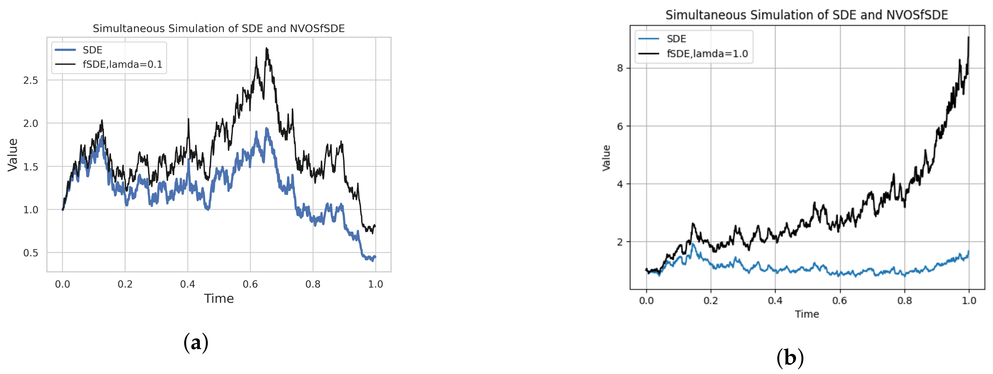
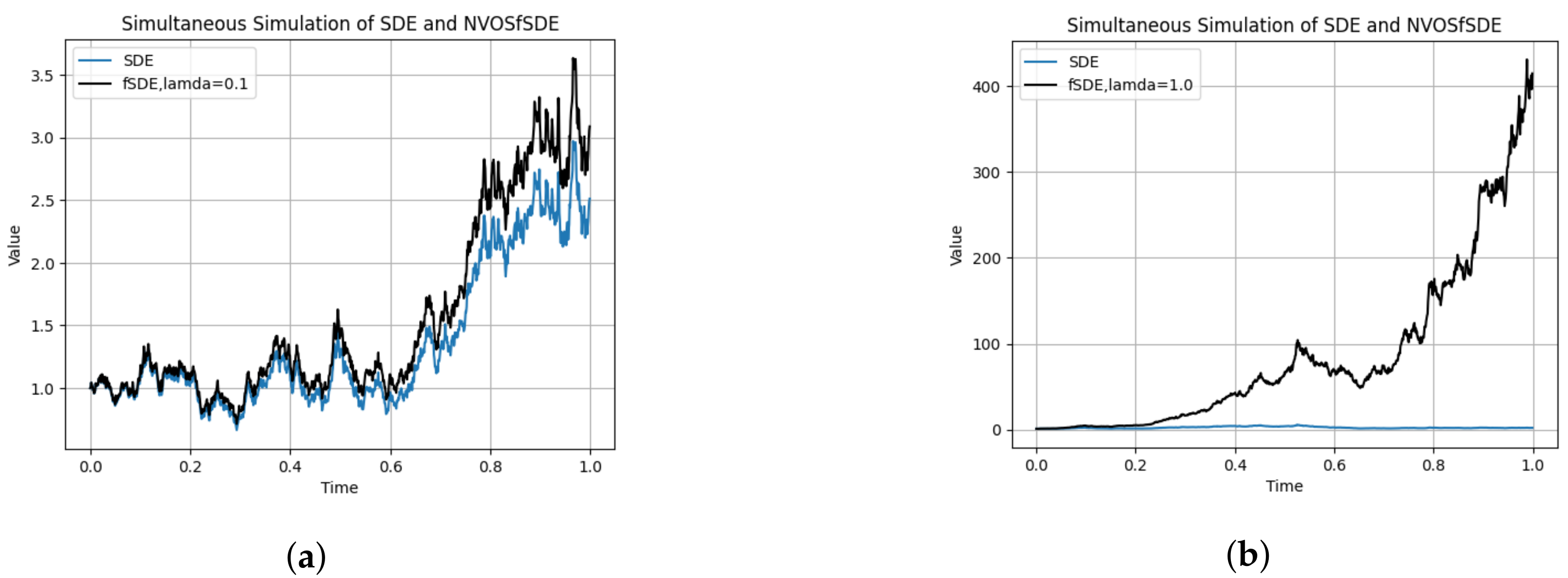
In Figure 1 and Figure 2 below, we show the results for , respectively. Each figure shows the plots with values between . We note that the FSDE solution (2) and the standard SDE solution are nearly identical for (here in this case). In contrast to , the FSDE solution (2) exhibits a considerable difference from the SDE solution.
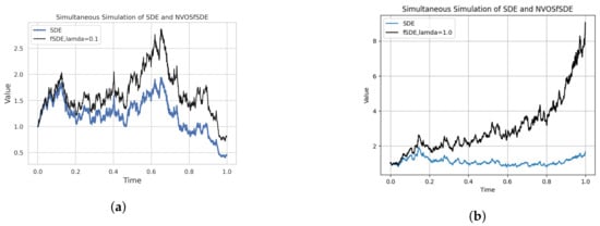
Figure 1.
Plots of SDE and FSDE solutions with the same sample size: classical SDE solutions (in blue) and the variable-order FSDE solutions (in black); (a) () = (0.2, 0.1) and ; (b) () = (0.2, 0.1) and .
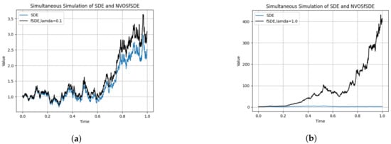
Figure 2.
Plots of SDE and FSDE solutions with the same sample size: classical SDE solutions (in blue) and the variable-order FSDE solutions (in black); (a) () = (0.8, 0.5) and ; (b) () = (0.8, 0.5) and .
5. Concluding Remarks
In this article, we investigate a non-Lipschitz non-singular kernel variable order fractional stochastic differential equation subjected to a nonlinear multiplicative white noise that loses the convolution structure due to the variable order fractional differential operator. In addition to the well-posedness and moment estimates of the problem, we developed and proved a generalized Euler–Maruyama scheme and showed the strong convergence of the EM approximation scheme.
In particular, the strong convergence results obtained in this paper had the same result as the classical stochastic differential equations when taking and in the variable-order FSDE; we obtained the results related to the classical version of the problem under consideration.
To support the theoretical findings, we conducted numerical experiments. In particular, when the variable-order FSDE is and , the behavior of the obtained convergence resembles the well-known convergence rates of the Euler–Maruyama scheme for conventional SDEs.
There are future perspectives and research potential directions which are mainly inspired from the need of sound mathematical analysis to extend the results obtained in this paper. We will mainly be interested in the question of global regularity and asymptotic expansion of the solutions for these SFPDEs. Additionally, many other open problems in this direction, such as the invariant measure and the ergodicity of the associated solutions, are crucial for future perspective work. The long-time behavior of a fractional stochastic system is of great relevance in long-term prediction of weather/climate or natural phenomena. Investigating the well-posedness of the the SFPDEs driven by Gaussian jumps and Levy processes and with non-regular intensity is still an open problem that can be addressed in future work.
Author Contributions
Conceptualization, Z.A. and M.A.A.; methodology, Z.A.; validation, T.N.; formal analysis, Z.A. and T.N.; resources, Z.A., M.A.A. and T.N.; writing—original draft preparation, Z.A. and M.A.A.; writing—review and editing, Z.A. and M.A.A.; supervision, T.N. All authors have read and agreed to the published version of the manuscript.
Funding
This research received no external funding.
Data Availability Statement
No data is used in this study.
Acknowledgments
We would like to express our gratitude and sincere and special thanks to the referees, whom valuable comments and suggestions greatly improved the quality of this manuscript.
Conflicts of Interest
The authors declare no conflicts of interest.
Appendix A
Definition A1
(Hlder and Lipschitz [57]). Let and be Banach spaces. A function is Hlder continuous with constant if there exists a constant such that
If the above holds with , then u is said to be Lipschitz continuous or globally Lipschitz continuous just to stress that L is uniform for .
Definition A2
(Euclidean norm). The Euclidean norm(simply norm) function on a coordinate space is defined by
Definition A3
(Progressively measurable). A stochastic process defined on a filtered probability space is progressively measurable with respect to, if the function is measurable for every .
Definition A4
(Adapted). A stochastic process on is adapted to the filtration or -adapted if for each .
Definition A5
(Mittag-Leffler function). The exponential function plays a crucial role in the theory of integer-order differential equations.
- (i)
- A one-parameter function of the Mittag-Leffler function type is defined in [58] by setting
- (ii)
- A two-parameter function of Mittag-Leffler function type is defined in [58] by setting
Lemma A1.
Let and . Then, for any and , it holds that
Proof.
From Lemma A1 of [59] and by Assumption (8), we have
Inserting (A4) into (10), we then deduce from the resulting relation that
Therefore,
□
Lemma A2.
(The Burkhlder–Davis–Gundy inequality [33,60,61]). If Y is a continuous martingale on , then there exists a positive constant for such that
Lemma A3.
(Generalized Gronwall inequality [33,62]). Let be a locally integrable non-negative and non-decreasing function on and σ be a non-negative constant. Suppose is a non-negative locally integrable function on with
then
Lemma A4.
(A Generalized discrete Gronwall’s inequality [33]). Suppose that a non-negative sequence and non-decreasing sequence satisfy the following relation:
Then the sequence can be bounded from above by
Lemma A5.
((Jensen’s inequality) [33]). If , then
References
- Diethelm, K.; Ford, N.J. The analysis of fractional differential equations. In Lecture Notes in Mathematics; Springer: Berlin/Heidelberg, Germany, 2004. [Google Scholar]
- Gulgowski, J.; Stefański, T.P. On applications of fractional derivatives in electromagnetic theory. In Proceedings of the 23rd International Microwave and Radar Conference (MIKON), Warsaw, Poland, 5–8 October 2020; pp. 13–17. [Google Scholar]
- Gulgowski, J.; Stefański, T.P.; Trofimowicz, D. On applications of elements modelled by fractional derivatives in circuit theory. Energies 2020, 13, 5768. [Google Scholar] [CrossRef]
- Hilfer, R. Mathematical and physical interpretations of fractional derivatives and integrals. In Handbook of Fractional Calculus with Applications 1; De Gruyter: Berlin, Germany, 2019; pp. 47–85. [Google Scholar]
- Kilbas, A.A.; Srivastava, H.M.; Trujillo, J.J. Theory and Applications of Fractional Differential Equations; Elsevier: Amsterdam, The Netherlands, 2006; Volume 204. [Google Scholar]
- Uchaikin, V.V. Fractional Derivatives for Physicists and Engineers; Springer: Berlin/Heidelberg, Germany, 2013; Volume 2. [Google Scholar]
- Kaltenbacher, B.; Rundell, W. Some inverse problems for wave equations with fractional derivative attenuation. Inverse Probl. 2021, 37, 045002. [Google Scholar] [CrossRef]
- Zhou, Y. Fractional Evolution Equations and Inclusions: Analysis and Control; Academic Press: Cambridge, MA, USA, 2016. [Google Scholar]
- Duan, Y.; Jiang, Y.; Wei, Y.; Zhou, J. The solution of stochastic evolution equation with the fractional derivative. Phys. Scr. 2024, 99, 025219. [Google Scholar] [CrossRef]
- Bashar, M.H.; Ghosh, S.; Rahman, M.M. Dynamical exploration of optical soliton solutions for M-fractional Paraxial wave equation. PLoS ONE 2024, 19, e0299573. [Google Scholar] [CrossRef]
- Aksoy, E.; Kaplan, M.; Bekir, A. Exponential rational function method for space–time fractional differential equations. Waves Random Complex Media 2016, 26, 142–151. [Google Scholar] [CrossRef]
- Ghany, H.A.; Hyder, A.A.; Zakarya, M. Exact solutions of stochastic fractional Korteweg de-Vries equation with conformable derivatives. Chin. Phys. B 2020, 29, 030203. [Google Scholar] [CrossRef]
- Han, T.; Li, Z.; Wen, J.; Yuan, J. Classification of All Single Traveling Wave Solutions of (3 + 1)-Dimensional Jimbo-Miwa Equation with Space-Time Fractional Derivative. Adv. Math. Phys. 2022, 2022, 2466900. [Google Scholar] [CrossRef]
- Zou, G.A.; Wang, B. Stochastic Burgers’ equation with fractional derivative driven by multiplicative noise. Comput. Math. Appl. 2017, 74, 3195–3208. [Google Scholar] [CrossRef]
- Abu-Shady, M.; Kaabar, M.K. A generalized definition of the fractional derivative with applications. Math. Probl. Eng. 2021, 2021, 9444803. [Google Scholar] [CrossRef]
- Mohammed, W.W.; Iqbal, N.; Albalahi, A.M.; Abouelregal, A.E.; Atta, D.; Ahmad, H.; El-Morshedy, M. Brownian motion effects on analytical solutions of a fractional-space long–short-wave interaction with conformable derivative. Results Phys. 2022, 35, 105371. [Google Scholar] [CrossRef]
- Martínez, F.; Kaabar, M.K. A Novel Theoretical Investigation of the Abu-Shady-Kaabar Fractional Derivative as a Modeling Tool for Science and Engineering. Comput. Math. Methods Med. 2022, 2022, 4119082. [Google Scholar] [CrossRef] [PubMed]
- Han, T.; Li, Z.; Zhang, K. Exact solutions of the stochastic fractional long—Short wave interaction system with multiplicative noise in generalized elastic medium. Results Phys. 2023, 44, 106174. [Google Scholar] [CrossRef]
- Han, T.; Zhao, Z.; Zhang, K.; Tang, C. Chaotic behavior and solitary wave solutions of stochastic-fractional Drinfel’d-Sokolov-Wilson equations with Brownian motion. Results Phys. 2023, 51, 106657. [Google Scholar] [CrossRef]
- Peng, C.; Zhao, L. Dynamic effects on traveling wave solutions of the space-fractional long-short-wave interaction system with multiplicative white noise. Results Phys. 2023, 53, 106931. [Google Scholar] [CrossRef]
- Singh, B.K.; Kumar, A. New approximate series solutions of conformable time-space fractional Fokker-Planck Equation via two efficacious techniques. Partial. Differ. Eq. Appl. Math. 2022, 6, 100451. [Google Scholar] [CrossRef]
- Kim, H.; Sakthivel, R.; Debbouche, A.; Torres, D.F. Traveling wave solutions of some important Wick-type fractional stochastic nonlinear partial differential equations. Chaos Solitons Fractals 2020, 131, 109542. [Google Scholar] [CrossRef]
- Guo, B.; Pu, X.; Huang, F. Fractional Partial Differential Equations and Their Numerical Solutions; World Scientific: Singapore, 2015. [Google Scholar]
- Stynes, M.; O’Riordan, E.; Gracia, J.L. Error analysis of a finite difference method on graded meshes for a time-fractional diffusion equation. Siam J. Numer. Anal. 2017, 55, 1057–1079. [Google Scholar] [CrossRef]
- Shu, J.; Li, P.; Zhang, J.; Liao, O. Random attractors for the stochastic coupled fractional Ginzburg-Landau equation with additive noise. J. Math. Phys. 2015, 56, 102702. [Google Scholar] [CrossRef]
- Guner, O.; Aksoy, E.; Bekir, A.; Cevikel, A.C. Different methods for (3 + 1)-dimensional space-time fractional modified KdV-Zakharov-Kuznetsov equation. Comput. Math. Appl. 2016, 71, 1259–1269. [Google Scholar] [CrossRef]
- Cresson, J.; Szafrańska, A. Comments on various extensions of the Riemann-Liouville fractional derivatives: About the Leibniz and chain rule properties. Commun. Nonlinear Sci. Numer. Simul. 2020, 82, 104903. [Google Scholar] [CrossRef]
- El-Nabulsi, A.R. Fractional derivatives generalization of Einstein’s field equations. Indian J. Phys. 2013, 87, 195–200. [Google Scholar] [CrossRef]
- El-Nabulsi, R.A. Modifications at large distances from fractional and fractal arguments. Fractals 2010, 18, 185–190. [Google Scholar] [CrossRef]
- El-Nabulsi, R.A. Gravitons in fractional action cosmology. Int. J. Theor. Phys. 2012, 51, 3978–3992. [Google Scholar] [CrossRef]
- Koeller, R. Applications of fractional calculus to the theory of viscoelasticity. J. Appl. Mech. 1984, 51, 299–307. [Google Scholar] [CrossRef]
- Pedjeu, J.C.; Ladde, G.S. Stochastic fractional differential equations: Modeling, method and analysis. Chaos Solitons Fractals 2012, 45, 279–293. [Google Scholar] [CrossRef]
- Yang, Z.; Zheng, X.; Zhang, Z.; Wang, H. Strong convergence of a Euler-Maruyama scheme to a variable-order fractional stochastic differential equation driven by a multiplicative white noise. Chaos Solitons Fractals 2021, 142, 110392. [Google Scholar] [CrossRef]
- Sakamoto, K.; Yamamoto, M. Initial value/boundary value problems for fractional diffusion-wave equations and applications to some inverse problems. J. Math. Anal. Appl. 2011, 382, 426–447. [Google Scholar] [CrossRef]
- Ahmadova, A.; Mahmudov, N.I. Strong convergence of a Euler—Maruyama method for fractional stochastic Langevin equations. Math. Comput. Simul. 2021, 190, 429–448. [Google Scholar] [CrossRef]
- Ding, X.L.; Nieto, J.J. Analytical solutions for multi-time scale fractional stochastic differential equations driven by fractional Brownian motion and their applications. Entropy 2018, 20, 63. [Google Scholar] [CrossRef]
- Doan, T.S.; Huong, P.T.; Kloeden, P.E.; Vu, A.M. Euler–Maruyama scheme for Caputo stochastic fractional differential equations. J. Comput. Appl. Math. 2020, 380, 112989. [Google Scholar] [CrossRef]
- Dong, J.; Du, N.; Yang, Z. A distributed-order fractional stochastic differential equation driven by Levy noise: Existence, uniqueness, and a fast EM scheme. Chaos: Interdiscip. J. Nonlinear Sci. 2023, 33, 023109. [Google Scholar] [CrossRef]
- Huang, J.; Shao, L.; Liu, J. Euler–Maruyama methods for Caputo tempered fractional stochastic differential equations. Int. J. Comput. Math. 2024, 2024, 1–19. [Google Scholar] [CrossRef]
- Li, X.; Yang, X. Error estimates of finite element methods for stochastic fractional differential equations. J. Comput. Math. 2017, 35, 346–362. [Google Scholar]
- Li, M.; Dai, X.; Huang, C. Fast Euler–Maruyama method for weakly singular stochastic Volterra integral equations with variable exponent. Numer. Algorithms 2023, 92, 2433–2455. [Google Scholar] [CrossRef]
- Xiao, A.; Dai, X.; Bu, W. Well-posedness and EM approximation for nonlinear stochastic fractional integro-differential equations with weakly singular kernels. arXiv 2019, arXiv:1901.10333. [Google Scholar]
- Yu, Y. Convergence of Relative Entropy for Euler-Maruyama Scheme to Stochastic Differential Equations with Additive Noise. Entropy 2024, 26, 232. [Google Scholar] [CrossRef]
- Zhang, J.; Tang, Y.; Huang, J. A fast Euler-Maruyama method for fractional stochastic differential equations. J. Appl. Math. Comput. 2023, 69, 273–291. [Google Scholar] [CrossRef]
- Abou-Senna, A.; Al Nemer, G.; Zhou, Y.; Tian, B. Convergence Rate of the Diffused Split-Step Truncated Euler–Maruyama Method for Stochastic Pantograph Models with Levy Leaps. Fractal Fract. 2023, 7, 861. [Google Scholar] [CrossRef]
- Agrawal, N.; Hu, Y. Jump models with delay—Option pricing and logarithmic Euler-Maruyama scheme. Mathematics 2020, 8, 1932. [Google Scholar] [CrossRef]
- Batiha, I.M.; Abubaker, A.A.; Jebril, I.H.; Al-Shaikh, S.B.; Matarneh, K. A numerical approach of handling fractional stochastic differential equations. Axioms 2023, 12, 388. [Google Scholar] [CrossRef]
- Wang, H.; Zheng, X. Wellposedness and regularity of the variable-order time-fractional diffusion equations. J. Math. Anal. Appl. 2019, 475, 1778–1802. [Google Scholar] [CrossRef]
- Zheng, X.; Zhang, Z.; Wang, H. Analysis of a nonlinear variable-order fractional stochastic differential equation. Appl. Math. Lett. 2020, 107, 106461. [Google Scholar] [CrossRef]
- Caputo, M.; Fabrizio, M. A new definition of fractional derivative without singular kernel. Progr. Fract. Differ. Appl. 2015, 1, 73–85. [Google Scholar]
- De Espíndola, J.J.; Bavastri, C.A.; de Oliveira Lopes, E.M. Design of optimum systems of viscoelastic vibration absorbers for a given material based on the fractional calculus model. J. Vib. Control. 2008, 14, 1607–1630. [Google Scholar] [CrossRef]
- Losada, J.; Nieto, J.J. Properties of a new fractional derivative without singular kernel. Progr. Fract. Differ. Appl. 2015, 1, 87–92. [Google Scholar]
- Pardoux, É. Equation Aux Derivees Partielles Stochastiques non Lineaires Monotones. PhD Thesis, Universite Paris, Paris, France, 1975. [Google Scholar]
- Nouri, K.; Ranjbar, H.; Torkzadeh, L. Solving the stochastic differential systems with modified split-step euler-maruyama method. Commun. Nonlinear Sci. Numer. Simul. 2020, 84, 105153. [Google Scholar] [CrossRef]
- Jia, J.; Yang, Z.; Wang, H. Analysis and numerical approximation for a nonlinear hidden-memory variable-order fractional stochastic differential equation. East Asian J. Appl. Math. 2022, 12, 673–695. [Google Scholar] [CrossRef]
- Jia, J.; Zheng, X.; Fu, H.; Dai, P.; Wang, H. A fast method for variable-order space-fractional diffusion equations. Numer. Algorithms 2020, 85, 1519–1540. [Google Scholar] [CrossRef]
- Lord, G.J.; Powell, C.E.; Shardlow, T. An Introduction to Computational Stochastic PDEs; Cambridge Texts in Applied Mathematics; Cambridge University Press: Cambridge, UK, 2014. [Google Scholar]
- Podlubny, I.; Thimann, K.V. (Eds.) Fractional Differential Equations: An Introduction to Fractional Derivatives, Fractional Differential Equations, to Methods of Their Solution and Some of Their Applications, 1st ed.; Mathematics in Science and Engineering 198; Academic Press: Cambridge, MA, USA, 1998. [Google Scholar]
- Zheng, X.; Wang, H.; Fu, H. Well-posedness of fractional differential equations with variable-order caputo-fabrizio derivative. Chaos Solitons Fractals 2020, 138, 109966. [Google Scholar] [CrossRef]
- Zhang, Z.; Karniadakis, G.E. Numerical Methods for Stochastic Partial Differential Equations with White Noise; Springer: Berlin/Heidelberg, Germany, 2017; Volume 196. [Google Scholar]
- Le Gall, J.F.; Le Gall, J.F. Brownian motion and partial differential equations. In Brownian Motion, Martingales, and Stochastic Calculus; Springer: Berlin/Heidelberg, Germany, 2016; pp. 185–208. [Google Scholar]
- Shao, J. New integral inequalities with weakly singular kernel for discontinuous functions and their applications to impulsive fractional differential systems. J. Appl. Math. 2014, 2014, 252946. [Google Scholar] [CrossRef]
Disclaimer/Publisher’s Note: The statements, opinions and data contained in all publications are solely those of the individual author(s) and contributor(s) and not of MDPI and/or the editor(s). MDPI and/or the editor(s) disclaim responsibility for any injury to people or property resulting from any ideas, methods, instructions or products referred to in the content. |
© 2024 by the authors. Licensee MDPI, Basel, Switzerland. This article is an open access article distributed under the terms and conditions of the Creative Commons Attribution (CC BY) license (https://creativecommons.org/licenses/by/4.0/).