General Solutions for MHD Motions of Ordinary and Fractional Maxwell Fluids through Porous Medium When Differential Expressions of Shear Stress Are Prescribed on Boundary

Abstract

Some MHD unidirectional motions of the electrically conducting incompressible Maxwell fluids between infinite horizontal parallel plates incorporated in a porous medium are analytically and graphically investigated when differential expressions of the non-trivial shear stress are prescribed on the boundary. Such boundary conditions are usually necessary in order to formulate well-posed boundary value problems for motions of rate-type fluids. General closed-form expressions are established for the dimensionless fluid velocity, the corresponding shear stress, and Darcy’s resistance. For completion, as well as for comparison, all results are extended to a fractional model of Maxwell fluids in which the time fractional Caputo derivative is used. It is proven for the first time that a large class of unsteady motions of the fractional incompressible Maxwell fluids becomes steady in time. For illustration, three particular motions are considered, and the correctness of the results is graphically proven. They correspond to constant or oscillatory values of the differential expression of shear stress on the boundary. In the first case, the required time to reach the steady state is graphically determined. This time declines for increasing values of the fractional parameter. Consequently, the steady state is reached earlier for motions of the ordinary fluids in comparison with the fractional ones. Finally, the fluid velocity, shear stress, and Darcy’s resistance are graphically represented and discussed for the fractional model.

1. Introduction

Incompressible Maxwell fluids (IMFs), which are relevant when modelling the behaviour of some polymers [1], were initially developed by Maxwell [2] to describe the viscous and elastic responses of air. They form the simplest class of rate-type fluids that take into consideration the relaxation phenomenon and have been used to study viscoelastic flows for both small and large values of the dimensionless time of relaxation. The constitutive equations of these fluids are given by the following relations [3].

$$\mathit{T}=-p\mathit{I}+{\mathit{T}}_E,\hspace{1em}{\mathit{T}}_E+\lambda \left(\frac{d{\mathit{T}}_E}{dt}-\mathit{L}{\mathit{T}}_E-{\mathit{T}}_E{\mathit{L}}^T\right)=2\mu \mathit{D}\hspace{0.17em}.$$

(1)

Here T is the stress tensor, ${\mathit{T}}_E$ is the extra-stress tensor, L is the velocity gradient, D is the rate of deformation tensor, $-p\mathit{I}$ represents the indeterminate stress due to the constraint of incompressibility, $\lambda$ is the relaxation time of the fluid and $\mu$ is the fluid viscosity. If $\lambda =0$, the governing Equation (1) define the incompressible Newtonian fluids.

In the literature there are numerous studies regarding unsteady motions of Maxwell fluids using different techniques and the exact solutions for such motions are important from two points of view. Firstly, they serve as descriptions of the behavior of those fluids in different circumstances and secondly, they can be useful to verify numerical procedures that are developed for more complex motion problems. The first exact solutions for unsteady motions of incompressible Maxwell fluids seem to be those of Srivastava [4] in cylindrical domains. Recently, steady state solutions for two oscillatory flows of these fluids through a tube with rectangular cross section or isosceles right triangular cross section were obtained by Wang et al. [5] and Sun et al. [6], respectively. Analytical solutions for unsteady motions of same fluids in rectangular domains can be found, for instance, in the book of Bohme [3], and the paper of Hayat et al. [7].

In the last decades the fractional calculus has been successfully used in describing of complex dynamic [8,9], it being a valuable tool to handle viscoelastic properties of fluids. A good fit of experimental data with theoretical results has been achieved by Makris [10,11] using the fractional Maxwell model instead of the classical model of Maxwell fluids. To describe rheological characteristics of many materials, constitutive equations with fractional derivatives have been proposed by Bagley [12], Friedrich [13], Mainardi [14] and Hristov [15]. Among the first exact solutions for unsteady motions of the fractional incompressible Maxwell fluids (FIMFs) over an infinite plate or between two infinite parallel plates we remember those of Tan and Xu [16], Tan et al. [17], Hayat et al. [18], Shaowei and Mingyu [19], Qi and Xu [20] and Corina Fetecau et al. [21].

At the same time, the fluid motions in the presence of a magnetic field or through a porous medium have multiple applications in polymer technology, the petroleum industry, nuclear reactors, geophysical and astrophysical studies, oil reservoir technology, agricultural engineering, and many other fields. The interference between a moving electrical conducting fluid and a magnetic field produces effects with applications in chemistry, physics, and engineering. The most recent works that have studied such motions of electrically conducting incompressible Maxwell fluids (ECIMFs) between infinite parallel plates are those of Ullah et al. [22] and Fetecau et al. [23]. However, none of the above-mentioned papers have studied the motions of ECIMFs in which a differential expression of shear stress is prescribed on the boundary. Foundationally, Renardy [24,25] brought to light the fact that differential expressions of stresses have to be prescribed on the boundary in order to formulate well-posed boundary value problems for rate-type fluids. The first exact steady solutions for MHD motions of a large class of rate fluids through a porous medium have been recently provided by Fetecau et al. [26].

The main purpose of the present work was to investigate some unidirectional MHD motions of ECIMFs between two infinite horizontal parallel plates incorporated in a porous medium when differential expressions of the non-trivial shear stress are prescribed on the boundary. For extension, as well as for comparison with a fractional model, general dimensionless solutions corresponding to the same motions of the fractional electrically conducting incompressible Maxwell fluids (FECIMFs) were also determined. In both situations, closed-form expressions were established for the fluid velocity, non-trivial shear stress, and Darcy’s resistance. It was proven that, in some circumstances, the unsteady motions of FECIMFs become steady in time. For illustration, as well as for comparison, three particular cases were considered, and the correctness of the obtained results was graphically proved. Finally, some characteristics of the FECIMFs’ behaviours were graphically underlined and discussed.

2. Presentation of the Problem

Consider an ECIMF at rest between two infinite horizontal parallel plates embedded in a porous medium. At this moment $\tilde{t}=0^{+}$, the two plates begin to apply time-dependent shear stresses of the form (see Figure 1).

Figure 1. Flow geometry.

$$\tilde{\eta }(0,\tilde{t})=\frac{S}{\lambda }{\displaystyle \underset{0}{\overset{\tilde{t}}{\int }}{h}_{\mathcal{l}}\left(\tau \right)}\exp \left(-\frac{\tilde{t}-\tau }{\lambda }\right)d\tau ,\hspace{1em}\tilde{\eta }(H,\tilde{t})=\frac{S}{\lambda }{\displaystyle \underset{0}{\overset{\tilde{t}}{\int }}{h}_u\left(\tau \right)}\exp \left(-\frac{\tilde{t}-\tau }{\lambda }\right)d\tau ;\hspace{0.17em}\hspace{0.17em}\hspace{0.17em}\tilde{t}>0,$$

(2)

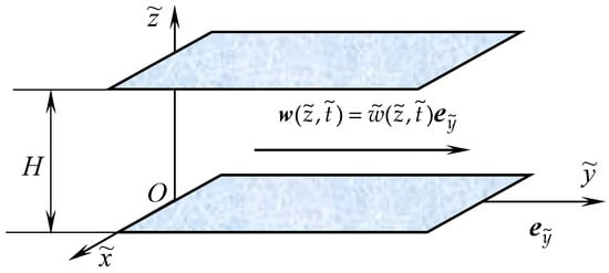to the fluid and a uniform magnetic field of magnitude B acts vertically on plates. Here, S is a constant shear stress, while the two functions $h_{\mathcal{l}}(\cdot )$ and $h_u(\cdot )$ are piecewise continuous $h_{\mathcal{l}}(0)=h_u(0)=0$. We also assume that the fluid is finitely conducting and its magnetic Reynolds number is small enough. So, the Joule heating and the induced magnetic field can be neglected. The ionized liquids and the fluids exhibiting metallic properties, for instance, satisfy these conditions [27]. Furthermore, the Hall effects will be neglected for moderate values of the Hartmann number.

Due to the shear, the fluid is gradually moved, and its movement in a suitable Cartesian coordinate system $\tilde{x},\hspace{0.17em}\hspace{0.17em}\tilde{y}$, and $\tilde{z}$, the $\tilde{z}$-axis of which is vertical to plates, is characterized by the velocity vector [3,7]

$$\mathit{w}=\mathit{w}(\tilde{z},\tilde{t})=\tilde{w}(\tilde{z},\tilde{t}){\mathit{e}}_{\tilde{y}}.$$

(3)

Here ${\mathit{e}}_{\tilde{y}}$ is the unit vector along the $\tilde{y}$-axis and the continuity equation is identically satisfied. We also assume that the extra-stress tensor S, as well as the fluid velocity, is a function of $\tilde{z}$ and $\tilde{t}$ only, and no superfluous electric charge exists. In these conditions, the balance of linear momentum reduces to a partial differential equation [28]

$$\rho \frac{\mathsf{\partial }\tilde{w}(\tilde{z},\tilde{t})}{\mathsf{\partial }\tilde{t}}=\frac{\mathsf{\partial }\tilde{\eta }(\tilde{z},\tilde{t})}{\mathsf{\partial }\tilde{z}}-\sigma B^2\tilde{w}(\tilde{z},\tilde{t})+\tilde{R}(\tilde{z},\tilde{t});\hspace{1em}\tilde{z}\in (0,H),\hspace{0.17em}\hspace{0.17em}\tilde{t}>0,$$

(4)

if there is no pressure gradient in the flow direction. In the previous relation, $\rho$ is the fluid density, $\sigma$ is its electrical conductivity, $\tilde{\eta }(\tilde{z},\tilde{t})={\tilde{S}}_{\tilde{y} \tilde{z}}(\tilde{z},\tilde{t})$ is the non-trivial shear stress, H is the distance between plates, and Darcy’s resistance $\tilde{R}(\tilde{z},\tilde{t})$ has to satisfy the following partial differential equation [28]

$$\left(1+\lambda \frac{\mathsf{\partial }}{\mathsf{\partial }\tilde{t}}\right)\tilde{R}(\tilde{z},\tilde{t})=-\mu \frac{\varphi }{k}\tilde{w}(\tilde{z},\tilde{t});\hspace{1em}\tilde{z}\in (0,H),\hspace{0.17em}\hspace{0.17em}\tilde{t}>0,$$

(5)

in which $\varphi$ is the porosity and k is the permeability of the porous medium.

Introducing $\tilde{\mathit{w}}(\tilde{z},\tilde{t})$ Equation (3) into the second relation (1), and bearing in mind the fact that the fluid has been at rest up to the initial moment $\tilde{t}=0$, results in the non-trivial tangential stress $\tilde{\eta }(\tilde{z},\tilde{t})$ having to satisfy the partial differential equation.

$$\left(1+\lambda \frac{\mathsf{\partial }}{\mathsf{\partial }\tilde{t}}\right)\tilde{\eta }(\tilde{z},\tilde{t})=\mu \frac{\mathsf{\partial }\tilde{w}(\tilde{z},\tilde{t})}{\mathsf{\partial }\tilde{z}};\hspace{1em}\tilde{z}\in (0,H),\hspace{0.17em}\hspace{0.17em}\tilde{t}>0.$$

(6)

In the above relation, $\varphi$ and k are the porosity and the permeability, respectively, of the porous medium.

The appropriate initial and boundary conditions are

$$\tilde{w}(\tilde{z},0)=0,\hspace{0.17em}\hspace{0.17em}\hspace{0.17em}\tilde{\eta }(\tilde{z},0)=0,\hspace{0.17em}\hspace{0.17em}\hspace{0.17em}\tilde{R}(\tilde{z},0)=0;\hspace{1em}\tilde{z}\in (0,H),$$

(7)

$$\begin{array}{l}\left(1+\lambda \frac{\mathsf{\partial }}{\mathsf{\partial }\tilde{t}}\right)\tilde{\eta }(0,\tilde{t})=\mu {\left.\frac{\mathsf{\partial }\tilde{w}(\tilde{z},\tilde{t})}{\mathsf{\partial }\tilde{z}}\right|}_{\tilde{z}=0}=S{h}_{\mathcal{l}}(\tilde{t});\hspace{1em}\tilde{t}>0,\\ \left(1+\lambda \frac{\mathsf{\partial }}{\mathsf{\partial }\tilde{t}}\right)\tilde{\eta }(H,\tilde{t})=\mu {\left.\frac{\mathsf{\partial }\tilde{w}(\tilde{z},\tilde{t})}{\mathsf{\partial }\tilde{z}}\right|}_{\tilde{z}=H}=S{h}_u(\tilde{t});\hspace{1em}\tilde{t}>0.\end{array}$$

(8)

The above relations (8) results in those differential expressions of the shear stress $\tilde{\eta }(\tilde{z},\tilde{t})$ being prescribed on the boundary. General exact solutions for such motion problems of ECIMFs are lacking in the literature. The volume flux $\tilde{Q}(\tilde{t})$ across a plane perpendicular to the flow direction per unit width of this plane can be determined by means of the following relation

$$\tilde{Q}(\tilde{t})={\displaystyle \underset{0}{\overset{H}{\int }}\tilde{w}(\tilde{z},\tilde{t})d\tilde{z};\hspace{1em}\tilde{t}>0.}$$

(9)

Introducing the following non-dimensional functions and variables

$$w=\frac{\mu }{SH}\tilde{w},\hspace{0.17em}\hspace{0.17em}\hspace{0.17em}\eta =\frac{1}{S}\tilde{\eta },\hspace{0.17em}\hspace{0.17em}\hspace{0.17em}R=\frac{H}{S}\tilde{R},\hspace{0.17em}\hspace{0.17em}\hspace{0.17em}Q=\frac{S{H}^2}{\mu }\tilde{Q},\hspace{0.17em}\hspace{0.17em}z=\frac{1}{H}\tilde{z},\hspace{0.17em}\hspace{0.17em}\hspace{0.17em}t=\frac{\nu }{H^2}\tilde{t},\hspace{0.17em}\hspace{0.17em}\hspace{0.17em}$$

(10)

where $\nu =\mu /\rho$ is the kinematic viscosity of the fluid, one obtains the dimensionless forms

$$\frac{\mathsf{\partial }w(z,t)}{\mathsf{\partial }t}=\frac{\mathsf{\partial }\eta (z,t)}{\mathsf{\partial }z}-{\mathrm{Ha}}^{2}w(z,t)+R(z,t);\hspace{0.17em}\hspace{0.17em}\hspace{0.17em}z\in (0,1),\hspace{0.17em}\hspace{0.17em}\hspace{0.17em}t>0,$$

(11)

$$\left(1+\mathrm{We}\frac{\mathsf{\partial }}{\mathsf{\partial }t}\right)R(z,t)=-Kw(z,t);\hspace{0.17em}\hspace{0.17em}\hspace{0.17em}z\in (0,1),\hspace{0.17em}\hspace{0.17em}\hspace{0.17em}t>0,$$

(12)

$$\left(1+\mathrm{We}\frac{\mathsf{\partial }}{\mathsf{\partial }t}\right)\eta (z,t)=\frac{\mathsf{\partial }w(z,t)}{\mathsf{\partial }z};\hspace{0.17em}\hspace{0.17em}\hspace{0.17em}z\in (0,1),\hspace{0.17em}\hspace{0.17em}\hspace{0.17em}t>0,$$

(13)

for the three governing Equations (4)–(6). In these last equations, the Hartmann and Weissenberg numbers Ha and We, respectively, and the porosity parameter K are defined by the following relations

$$\mathrm{Ha}=BH\sqrt{\frac{\sigma }{\mu }},\hspace{0.17em}\hspace{0.17em}\hspace{0.17em}\mathrm{We}=\frac{\lambda }{t_0},\hspace{0.17em}\hspace{0.17em}\hspace{0.17em}K=\frac{\varphi }{k}{H}^2,$$

(14)

where $t_0=H^2/\nu$ is a characteristic time scale. The Hartman number is the ratio of electromagnetic force to the viscous force, while the Weissenberg number is the ratio of the relaxation time and a characteristic time scale.

The corresponding initial and boundary conditions are

$$w(z,0)=0,\hspace{0.17em}\hspace{0.17em}\hspace{0.17em}\eta (z,0)=0,\hspace{0.17em}\hspace{0.17em}\hspace{0.17em}R(z,0)=0;\hspace{1em}z\in (0,1),$$

(15)

$${\left.\frac{\mathsf{\partial }w(z,t)}{\mathsf{\partial }z}\right|}_{z=0}=h_{\mathcal{l}}(t),\hspace{0.17em}\hspace{0.17em}{\left.\frac{\mathsf{\partial }w(z,t)}{\mathsf{\partial }z}\right|}_{z=1}=h_u(t)\hspace{0.17em};\hspace{1em}t>0.$$

(16)

The dimensionless volume flux $Q(t)$ can be determined using the relation

$$Q(t)={\displaystyle \underset{0}{\overset{1}{\int }}w(z,t)}dz;\hspace{1em}t>0.$$

(17)

In the following section, exact solutions for the system of partial differential Equations (11)–(13) with the initial and boundary conditions (15) and (16) will be derived by means of Laplace and finite Fourier cosine transforms. For illustration, as well as for the validation of obtained results, some special cases are considered, and equivalent forms are provided for the steady-state components of the starting velocities.

Later, for extension, exact general solutions will be established for the same motions of the fractional model described using Equation (11) and

$$\left(1+\mathrm{We}{\hspace{0.17em}}^{\mathrm{C}}{D}_t^{\alpha }\right) \eta (z,t)=\frac{\mathsf{\partial }w(z,t)}{\mathsf{\partial }z};\hspace{0.17em}z\in (0,1),\hspace{0.17em}t>0,$$

(18)

$$\left(1+\mathrm{We}{\hspace{0.17em}}^{\mathrm{C}}{D}_t^{\alpha }\right)R(z,t)=-Kw(z,t);\hspace{0.17em}\hspace{0.17em}\hspace{0.17em}z\in (0,1),\hspace{0.17em}\hspace{0.17em}\hspace{0.17em}t>0.$$

(19)

Their correctness will be proven by comparing them with the previous solutions, and the fluids whose behaviour can be described by the governing Equations (11), (18), and (19) will be called fractional electrically conducting incompressible Maxwell fluids (FECIMFs). The fractional Caputo derivative ${}^{\mathrm{C}}{D}_t^{\alpha }$ from the above equations is defined by the relation

$${}^{\mathrm{C}}{D}_t^{\alpha } \chi (z,t)=\left\{\begin{array}{l}\frac{1}{\Gamma (1-\alpha )}{\displaystyle \underset{0}{\overset{t}{\int }}{(t-\tau )}^{-\alpha }}\frac{\mathsf{\partial }\chi (z,\tau )}{\mathsf{\partial }\tau }d\tau \hspace{1em}\mathrm{for}\hspace{1em}0\le \alpha <1\\ \frac{\mathsf{\partial }\chi (z,t)}{\mathsf{\partial }t}\hspace{1em}\mathrm{for}\hspace{1em}\alpha =1\end{array}\right.$$

(20)

Additionally, its Laplace transform is

$$L\left\{{}^{\mathrm{C}}{D}_t^{\alpha } \chi (z,t)\right\}=s^{\alpha }L\left\{\chi (z,t)\right\}-s^{\alpha -1}\chi (z,0); \hspace{1em}\alpha \in [0,1].$$

(21)

The corresponding initial and boundary conditions are given by Equations (15) and (16).

3. Exact General Solutions Corresponding to the Ordinary Model (ECIMFs)

Applying the Laplace transform to the governing equalities (11)–(13) and bearing in mind the initial conditions (15), one attains to the following relations

$$s\overline{w}(z,s)=\frac{\mathsf{\partial }\overline{\eta }(z,s)}{\mathsf{\partial }z}-{\mathrm{Ha}}^2\overline{w}(z,s)+\overline{R}(z,s);\hspace{0.17em}\hspace{0.17em}\hspace{0.17em}z\in (0,1),$$

(22)

$$\overline{\eta }(z,s)=\frac{1}{s\mathrm{We}+1}\frac{\mathsf{\partial }\overline{w}(z,s)}{\mathsf{\partial }z},\hspace{0.17em}\hspace{0.17em}\hspace{0.17em}\overline{R}(z,s)=-\frac{K}{s\mathrm{We}+1}\overline{w}(z,s)\hspace{0.17em};\hspace{0.17em}\hspace{0.17em}\hspace{0.17em}z\in (0,1),$$

(23)

where $\overline{w}(z,s),\hspace{0.17em}\overline{\eta }(z,s),\hspace{0.17em}\overline{R}(z,s)$ are Laplace transforms of $w(z,t),\hspace{0.17em}\hspace{0.17em}\eta (z,t),\hspace{0.17em}\hspace{0.17em}R(z,t)$, respectively, and s is the transform parameter.

By eliminating $\hspace{0.17em}\overline{\eta }(z,s)$ and $\overline{R}(z,s)$ between Equations (22) and (23), one obtains the following ordinary differential equation

$$\frac{{\mathsf{\partial }}^2\overline{w}(z,s)}{\mathsf{\partial }{z}^2}-a_1(s)\overline{w}(z,s)=0;\hspace{0.17em}\hspace{0.17em}\hspace{0.17em}z\in (0,1),$$

(24)

with the boundary conditions

$${\left.\frac{\mathsf{\partial }\overline{w}(z,s)}{\mathsf{\partial }z}\right|}_{z=0}={\overline{h}}_{\mathcal{l}}(s),\hspace{0.17em}\hspace{0.17em}\hspace{0.17em}\hspace{0.17em}{\left.\frac{\mathsf{\partial }\overline{w}(z,s)}{\mathsf{\partial }z}\right|}_{z=1}={\overline{h}}_u(s);\hspace{0.17em}\hspace{0.17em}\hspace{0.17em}z\in (0,1),$$

(25)

for $\overline{w}(z,s)$. In the last two relations, the function $a_1(\cdot )$ is given by the equality

$$a_1(s)=(s+{\mathrm{Ha}}^2)(s\mathrm{We}+1)+K,$$

(26)

while ${\overline{h}}_{\mathcal{l}}(s),$ ${\overline{h}}_u(s)$ are the Laplace transforms of $h_{\mathcal{l}}(t)$ and $h_u(t)$, respectively.

In order to present in suitable forms the problem solutions, we firstly make the following change for the unknown function

$$\overline{w}(z,s)=f_1(z){\overline{h}}_{\mathcal{l}}(s)+f_2(z){\overline{h}}_u(s)+\overline{u}(z,s);\hspace{0.17em}\hspace{0.17em}\hspace{0.17em}z\in (0,1),$$

(27)

where

$$f_1(z)=-\frac{1}{2}{z}^2+z,\hspace{0.17em}\hspace{0.17em}\hspace{0.17em}{f}_2(z)=\frac{1}{2}{z}^2;\hspace{0.17em}\hspace{0.17em}\hspace{0.17em}z\in (0,1).$$

(28)

Substituting $\overline{w}(z,s)$ from Equation (27) into (24), and having in mind the boundary conditions (25), results in the new function $\overline{u}(z,s)$ having to satisfy the ordinary differential equation

$$\frac{{\mathsf{\partial }}^2\overline{u}(z,s)}{\mathsf{\partial }{z}^2}-a_1(s)\overline{u}(z,s)=a_1(s)\left[f_1(z){\overline{h}}_{\mathcal{l}}(s)+f_2(z){\overline{h}}_u(s)\right]+{\overline{h}}_{\mathcal{l}}(s)-{\overline{h}}_u(s);\hspace{0.17em}\hspace{0.17em}\hspace{0.17em}z\in (0,1),$$

(29)

with the boundary conditions

$${\left.\frac{\mathsf{\partial }\overline{u}(z,s)}{\mathsf{\partial }z}\right|}_{z=0}=0,\hspace{0.17em}\hspace{0.17em}\hspace{0.17em}\hspace{0.17em}{\left.\frac{\mathsf{\partial }\overline{u}(z,s)}{\mathsf{\partial }z}\right|}_{z=1}=0.$$

(30)

The solution to the ordinary differential Equation (29) with the boundary conditions (30) will be determined by means of the finite Fourier cosine transform and its inverse defined by the relations (A1) from Appendix A. Consequently, by multiplying Equation (29) by $\cos ({\lambda }_{n}z)$, integrating the result between zero and one, and using the identities ((A2) and (A3)) from Appendix A, one finds the following expressions.

$${\overline{u}}_n(s)=\left\{\begin{array}{l}-\frac{1}{3}{\overline{h}}_{\mathcal{l}}(s)-\frac{1}{6}{\overline{h}}_u(s)+\frac{{\overline{h}}_u(s)-{\overline{h}}_{\mathcal{l}}(s)}{a_1(s)}\hspace{1em}\mathrm{for}\hspace{0.17em}\hspace{0.17em}\hspace{0.17em}\hspace{0.17em}n=0\\ \frac{{\overline{h}}_{\mathcal{l}}(s)+{(-1)}^{n+1}{\overline{h}}_u(s)}{{\lambda }_n^2[a_1(s)+{\lambda }_n^2]}{a}_1(s)\hspace{1em}\mathrm{for}\hspace{0.17em}\hspace{0.17em}\hspace{0.17em}\hspace{0.17em}n=1,2,3\dots \end{array}\right.$$

(31)

for the finite Fourier cosine transform ${\overline{u}}_n(s)$ of $\overline{u}(z,s)$. Here, ${\lambda }_n=n\pi$, where $n=1,2,3\dots$.

Here, by applying the inverse Fourier cosine transform to equality (31), one finds that

$$\overline{u}(z,s)=-\frac{1}{3}{\overline{h}}_{\mathcal{l}}(s)-\frac{1}{6}{\overline{h}}_u(s)+\frac{{\overline{h}}_u(s)-{\overline{h}}_{\mathcal{l}}(s)}{a_1(s)}+2{\displaystyle \sum _{n=1}^{\infty }\left[{\overline{h}}_{\mathcal{l}}(s)+{(-1)}^{n+1}{\overline{h}}_u(s)\right]}{A}_{1n}(s)\cos ({\lambda }_{n}z),$$

(32)

where

$$A_{1n}(s)=\frac{a_1(s)}{{\lambda }_n^2[a_1(s)+{\lambda }_n^2]};\hspace{0.17em}\hspace{0.17em}\hspace{0.17em}n=1,2,3\dots$$

(33)

By substituting $\overline{u}(z,s)$ from Equation (32) into (27), one obtains, for $\overline{w}(z,s)$, the expression

$$\begin{array}{l}\overline{w}(z,s)=\frac{1}{2}\left(z^2-\frac{1}{3}\right){\overline{h}}_u(s)-\left(\frac{1}{2}{z}^2-z+\frac{1}{3}\right){\overline{h}}_{\mathcal{l}}(s)+\frac{{\overline{h}}_u(s)-{\overline{h}}_{\mathcal{l}}(s)}{a_1(s)}\\ +2{\displaystyle \sum _{n=1}^{\infty }\left[{\overline{h}}_{\mathcal{l}}(s)+{(-1)}^{n+1}{\overline{h}}_u(s)\right]}{A}_{1n}(s)\cos ({\lambda }_{n}z);\hspace{0.17em}\hspace{0.17em}\hspace{0.17em}z\in (0,1).\end{array}$$

(34)

In order to determine the inverse Laplace transform of $1/a_1(s)$, we write it in the convenient form

$$\frac{1}{a_1(s)}=\frac{2}{\sqrt{\Delta }}\frac{\frac{\sqrt{\Delta }}{2\mathrm{We}}}{{\left(s+\frac{{\mathrm{Ha}}^2\mathrm{We}+1}{2\mathrm{We}}\right)}^2-{\left(\frac{\sqrt{\Delta }}{2\mathrm{We}}\right)}^2},$$

(35)

where $\Delta ={({\mathrm{Ha}}^2\mathrm{We}-1)}^2-4K\mathrm{We}.$ Using the identity (A4) from Appendix A, one finds that

$$L^{-1}\left\{\frac{1}{a_1(s)}\right\}=\frac{2}{\sqrt{\Delta }}\sinh \left(\frac{t\sqrt{\Delta }}{2\mathrm{We}}\right)\exp \left(-\frac{{\mathrm{Ha}}^2\mathrm{We}+1}{2\mathrm{We}}t\right).$$

(36)

Here, we write $A_{1n}(s)$ under the convenient form

$$A_{1n}(s)=\frac{1}{{\lambda }_n^2}-\frac{1}{a_1(s)+{\lambda }_n^2}=\frac{1}{{\lambda }_n^2}-\frac{1}{\mathrm{We}\sqrt{m^2-q_n^2}}\hspace{0.17em}\frac{\sqrt{m^2-q_n^2}}{{(s+r)}^2-{(\sqrt{m^2-q_n^2})}^2};\hspace{0.17em}\hspace{0.17em}\hspace{0.17em}n=1,2,3,\dots$$

(37)

where

$$m=\frac{{\mathrm{Ha}}^2\mathrm{We}-1}{2\mathrm{We}},\hspace{0.17em}\hspace{0.17em}\hspace{0.17em}{q}_n=\sqrt{\frac{K+{\lambda }_n^2}{\mathrm{We}}},\hspace{0.17em}\hspace{0.17em}\hspace{0.17em}r=\frac{{\mathrm{Ha}}^2\mathrm{We}+1}{2\mathrm{We}}$$

(38)

and apply the inverse Laplace transform. By using the identity (A4) from Appendix A one obtains

$$L^{-1}\left\{A_{1n}(s)\right\}=\frac{\delta (t)}{{\lambda }_n^2}-\frac{{\mathrm{e}}^{-rt}}{\mathrm{We}\sqrt{m^2-q_n^2}}\sinh \left(t\sqrt{m^2-q_n^2}\right)\hspace{0.17em},$$

(39)

where $\delta (\cdot )$ is the Dirac delta function.

Finally, by applying the inverse Laplace transform to Equation (34) and using the previous results, one finds for the dimensionless velocity field $w(z,t)$ the expression

$$\begin{array}{l}w(z,t)=\frac{1}{2}\left(z^2-\frac{1}{3}\right)h_u(t)-\left(\frac{1}{2}{z}^2-z+\frac{1}{3}\right)h_{\mathcal{l}}(t)+2{\displaystyle \sum _{n=1}^{\infty }\frac{h_{\mathcal{l}}(t)+{(-1)}^{n+1}{h}_u(t)}{{\lambda }_n^2}}\cos ({\lambda }_{n}z)\\ +\frac{2}{\sqrt{\Delta }}{\displaystyle \underset{0}{\overset{t}{\int }}\left[h_u(t-\tau )-h_{\mathcal{l}}(t-\tau )\right]}\hspace{0.17em}{\mathrm{e}}^{-r\tau }\sinh \left(\frac{\tau \sqrt{\Delta }}{2\mathrm{We}}\right)\hspace{0.17em}d\tau \\ -\frac{2}{\mathrm{We}}{\displaystyle \sum _{n=1}^{\infty }\frac{\cos ({\lambda }_{n}z)}{\sqrt{m^2-q_n^2}}{\displaystyle \underset{0}{\overset{t}{\int }}\left[h_{\mathcal{l}}(t-\tau )+{(-1)}^{n+1}{h}_u(t-\tau )\right]}}\hspace{0.17em}{\mathrm{e}}^{-r\tau }\sinh \left(\tau \sqrt{m^2-q_n^2}\right)d\tau ;\hspace{0.17em}\hspace{0.17em}\hspace{0.17em}z\in (0,1),\hspace{0.17em}\hspace{0.17em}t>0.\end{array}$$

(40)

The corresponding shear stress $\eta (z,t)$ and the Darcy’s resistance $R(z,t)$, which are given by the following two relations

$$\eta (z,t)=\frac{1}{\mathrm{We}}\frac{\mathsf{\partial }w(z,t)}{\mathsf{\partial }z}\ast {\mathrm{e}}^{-t/\mathrm{We}}=\frac{1}{\mathrm{We}}{\displaystyle \underset{0}{\overset{t}{\int }}\frac{\mathsf{\partial }w(z,\tau )}{\mathsf{\partial }z}{\mathrm{e}}^{-(t-\tau )/\mathrm{We}}}d\tau ;\hspace{0.17em}\hspace{0.17em}\hspace{0.17em}z\in (0,1),\hspace{0.17em}\hspace{0.17em}t>0,$$

(41)

$$R(z,t)=-\frac{K}{\mathrm{We}}w(z,t)\ast {\mathrm{e}}^{-t/\mathrm{We}}=-\frac{K}{\mathrm{We}}{\displaystyle \underset{0}{\overset{t}{\int }}w(z,\tau ){\mathrm{e}}^{-(t-\tau )/\mathrm{We}}}d\tau ;\hspace{0.17em}\hspace{0.17em}\hspace{0.17em}z\in (0,1),\hspace{0.17em}\hspace{0.17em}t>0,$$

(42)

have been obtained applying the Laplace transform and then its inverse to Equations (12) and (13).

In the special case when $h_{\mathcal{l}}(t)=h_u(t)=h(t)$ (when the two plates apply the same shear stress to the fluid) the corresponding velocity field $w(z,t)$ takes the simpler form (see for instance [29], the entry 3 of Table 8)

$$w(z,t)=-\frac{4}{\mathrm{We}}{\displaystyle \sum _{n=1}^{\infty }\frac{\cos ({\lambda }_{2n-1}z)}{\sqrt{m^2-q_{2n-1}^2}}}{\displaystyle \underset{0}{\overset{t}{\int }}h(t-\tau )}\hspace{0.17em}{\mathrm{e}}^{-r\tau }\sinh \left(\tau \sqrt{m^2-q_{2n-1}^2}\right)\hspace{0.17em}d\tau ;\hspace{0.17em}\hspace{0.17em}\hspace{0.17em}z\in (0,1),\hspace{0.17em}\hspace{0.17em}t>0.$$

(43)

3.1. Special Cases $h_{\mathcal{l}}(t)=h_u(t)=H(t)\cos (\omega t)$ and $h_{\mathcal{l}}(t)=h_u(t)=H(t)\sin (\omega t)$

Let us now consider the cases when the function $h(t)$ from Equation (43) is equal to $H(t)\cos (\omega t)$ or $H(t)\sin (\omega t)$, where $\omega$ is the non-dimensional frequency of the oscillations and $H(\cdot )$ is the Heaviside unit step function, and denote, using $w_c(z,t)$ and $w_s(z,t)$, the dimensionless starting velocities corresponding to the two associated motions. They are given by the relations.

$$w_c(z,t)=-\frac{4}{\mathrm{We}}{\displaystyle \sum _{n=1}^{\infty }\frac{\cos ({\lambda }_{2n-1}z)}{\sqrt{m^2-q_{2n-1}^2}}}{\displaystyle \underset{0}{\overset{t}{\int }}{\mathrm{e}}^{-r\tau }\sinh \left(\tau \sqrt{m^2-q_{2n-1}^2}\right)\hspace{0.17em}\hspace{0.17em}\cos [\omega (t-\tau )]}d\tau ;\hspace{0.17em}\hspace{0.17em}z\in (0,1),\hspace{0.17em}\hspace{0.17em}t>0,$$

(44)

$$w_s(z,t)=-\frac{4}{\mathrm{We}}{\displaystyle \sum _{n=1}^{\infty }\frac{\cos ({\lambda }_{2n-1}z)}{\sqrt{m^2-q_{2n-1}^2}}}{\displaystyle \underset{0}{\overset{t}{\int }}{\mathrm{e}}^{-r\tau }\sinh \left(\tau \sqrt{m^2-q_{2n-1}^2}\right)\hspace{0.17em}\hspace{0.17em}\sin [\omega (t-\tau )]}d\tau ;\hspace{0.17em}\hspace{0.17em}z\in (0,1),\hspace{0.17em}\hspace{0.17em}t>0.$$

(45)

Lengthy but straightforward computations show that the starting velocities $w_c(z,t)$$w_s(z,t)$ can be written as a summation of their steady-state (permanent or long time) and transient components, namely,

$$w_c(z,t)=w_{cp}(z,t)+w_{ct}(z,t),\hspace{0.17em}\hspace{0.17em}\hspace{0.17em}{w}_s(z,t)=w_{sp}(z,t)+w_{st}(z,t);\hspace{0.17em}\hspace{0.17em}\hspace{0.17em}z\in (0,1),\hspace{0.17em}\hspace{0.17em}t>0,$$

(46)

in which

$$\begin{array}{l}{w}_{cp}(z,t)=\frac{4}{\mathrm{We}}\cos (\omega t){\displaystyle \sum _{n=1}^{\infty }\frac{{\omega }^2+b_{2n-1}^2-r^2}{{({\omega }^2+b_{2n-1}^2-r^2)}^2+{(2r\omega )}^2}\cos ({\lambda }_{2n-1}z)}\\ -\frac{8r\omega }{\mathrm{We}}\sin (\omega t){\displaystyle \sum _{n=1}^{\infty }\frac{\cos ({\lambda }_{2n-1}z)}{{({\omega }^2+b_{2n-1}^2-r^2)}^2+{(2r\omega )}^2}};\hspace{0.17em}\hspace{0.17em}\hspace{0.17em}z\in (0,1),\hspace{0.17em}\hspace{0.17em}t\in R,\end{array}$$

(47)

$$\begin{array}{l}{w}_{ct}(z,t)=\frac{4r}{\mathrm{We}}{\mathrm{e}}^{-rt}{\displaystyle \sum _{n=1}^{\infty }\frac{r^2+{\omega }^2-b_{2n-1}^2}{{({\omega }^2+b_{2n-1}^2-r^2)}^2+{(2r\omega )}^2}\frac{\sinh (b_{2n-1}t)}{b_{2n-1}}\cos ({\lambda }_{2n-1}z)}\\ -\frac{4}{\mathrm{We}}{\mathrm{e}}^{-rt}{\displaystyle \sum _{n=1}^{\infty }\frac{{\omega }^2+b_{2n-1}^2-r^2}{{({\omega }^2+b_{2n-1}^2-r^2)}^2+{(2r\omega )}^2}}\cosh (b_{2n-1}t)\cos ({\lambda }_{2n-1}z);\hspace{0.17em}\hspace{0.17em}\hspace{0.17em}z\in (0,1),\hspace{0.17em}\hspace{0.17em}t>0,\end{array}$$

(48)

$$\begin{array}{l}{w}_{sp}(z,t)=\frac{8r\omega }{\mathrm{We}}\cos (\omega t){\displaystyle \sum _{n=1}^{\infty }\frac{\cos ({\lambda }_{2n-1}z)}{{({\omega }^2+b_{2n-1}^2-r^2)}^2+{(2r\omega )}^2}}\\ +\frac{4}{\mathrm{We}}\sin (\omega t){\displaystyle \sum _{n=1}^{\infty }\frac{{\omega }^2+b_{2n-1}^2-r^2}{{({\omega }^2+b_{2n-1}^2-r^2)}^2+{(2r\omega )}^2}\cos ({\lambda }_{2n-1}z)};\hspace{0.17em}\hspace{0.17em}\hspace{0.17em}z\in (0,1),\hspace{0.17em}\hspace{0.17em}t\in R,\end{array}$$

(49)

$$\begin{array}{l}{w}_{st}(z,t)=-\frac{4\omega }{\mathrm{We}}{\mathrm{e}}^{-rt}{\displaystyle \sum _{n=1}^{\infty }\frac{{\omega }^2+b_{2n-1}^2+r^2}{{({\omega }^2+b_{2n-1}^2-r^2)}^2+{(2r\omega )}^2}\frac{\sinh (b_{2n-1}t)}{b_{2n-1}}}\cos ({\lambda }_{2n-1}z)\\ -\frac{8r\omega }{\mathrm{We}}{\mathrm{e}}^{-rt}{\displaystyle \sum _{n=1}^{\infty }\frac{\cosh (b_{2n-1}t)}{{({\omega }^2+b_{2n-1}^2-r^2)}^2+{(2r\omega )}^2}}\cos ({\lambda }_{2n-1}z);\hspace{0.17em}\hspace{0.17em}\hspace{0.17em}z\in (0,1),\hspace{0.17em}\hspace{0.17em}t>0,\end{array}$$

(50)

where $b_n=\sqrt{m^2-q_n^2}$.

Direct computations show that the steady-state velocity fields $w_{cp}(z,t)$ and $w_{sp}(z,t)$ can also be presented in simpler forms, namely,

$$w_{cp}(z,t)=\mathrm{Re}\left\{\frac{\sin \mathrm{h}[\gamma (z-1/2)]}{\gamma \hspace{0.17em}\cos \mathrm{h}(\gamma /2)}{\mathrm{e}}^{i\omega t}\right\};\hspace{0.17em}\hspace{0.17em}\hspace{0.17em}z\in (0,1),\hspace{0.17em}\hspace{0.17em}\hspace{0.17em}t\in R,$$

(51)

$$w_{sp}(z,t)=\mathrm{Im}\left\{\frac{\sin \mathrm{h}[\gamma (z-1/2)]}{\gamma \hspace{0.17em}\cos \mathrm{h}(\gamma /2)}{\mathrm{e}}^{i\omega t}\right\};\hspace{0.17em}\hspace{0.17em}\hspace{0.17em}z\in (0,1),\hspace{0.17em}\hspace{0.17em}\hspace{0.17em}t\in R,$$

(52)

where $\gamma =\sqrt{({\mathrm{Ha}}^2+i\omega )(1+i\omega \mathrm{We})+K}$. Figure 2 clearly show the equivalence of the expressions of $w_{cp}(z,t)$ and $w_{sp}(z,t)$ given by Equations (47), (51) and (49), (52), respectively.

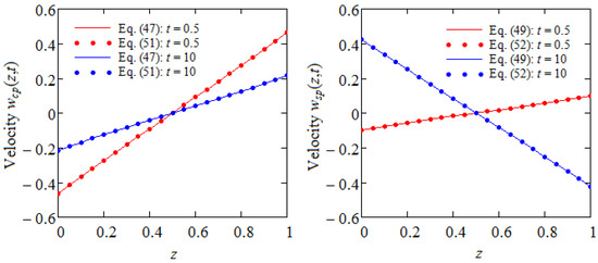
Figure 2. Equivalence of the expressions of $w_{cp}(z,t)$ and $w_{sp}(z,t)$ given by Equations (47), (51) and (49), (52), respectively, for $\omega =\pi /6,\hspace{0.17em}\hspace{0.17em}\mathrm{We}=0.8,$ $\mathrm{Ha}=0.5,\hspace{0.17em}\hspace{0.17em}K=0.6$ and two values of time t.

For completion, we also provide here the corresponding expressions for the steady state shear stresses ${\eta }_{cp}(z,t),\hspace{0.17em}\hspace{0.17em}{\eta }_{sp}(z,t)$ and the Darcy’s resistance $R_{cp}(z,t),\hspace{0.17em}\hspace{0.17em}{R}_{sp}(z,t)$, namely

$${\eta }_{cp}(z,t)=\mathrm{Re}\left\{\frac{\cos \mathrm{h}[\gamma (z-1/2)]}{\cos \mathrm{h}(\gamma /2)}\frac{{\mathrm{e}}^{i\omega t}}{1+i\omega \mathrm{We}}\right\};\hspace{0.17em}\hspace{0.17em}\hspace{0.17em}z\in (0,1),\hspace{0.17em}\hspace{0.17em}\hspace{0.17em}t\in R,$$

(53)

$${\eta }_{sp}(z,t)=\mathrm{Im}\left\{\frac{\cos \mathrm{h}[\gamma (z-1/2)]}{\cos \mathrm{h}(\gamma /2)}\frac{{\mathrm{e}}^{i\omega t}}{1+i\omega \mathrm{We}}\right\};\hspace{0.17em}\hspace{0.17em}\hspace{0.17em}z\in (0,1),\hspace{0.17em}\hspace{0.17em}\hspace{0.17em}t\in R,$$

(54)

$$R_{cp}(z,t)=-K\mathrm{Re}\left\{\frac{\sin \mathrm{h}[\gamma (z-1/2)]}{\gamma \cos \mathrm{h}(\gamma /2)}\frac{{\mathrm{e}}^{i\omega t}}{1+i\omega \mathrm{We}}\right\};\hspace{0.17em}\hspace{0.17em}\hspace{0.17em}z\in (0,1),\hspace{0.17em}t\in R,$$

(55)

$$R_{sp}(z,t)=-K\mathrm{Im}\left\{\frac{\sin \mathrm{h}[\gamma (z-1/2)]}{\gamma \cos \mathrm{h}(\gamma /2)}\frac{{\mathrm{e}}^{i\omega t}}{1+i\omega \mathrm{We}}\right\};\hspace{0.17em}\hspace{0.17em}\hspace{0.17em}z\in (0,1),\hspace{0.17em}\hspace{0.17em}\hspace{0.17em}t\in R.$$

(56)

Simple computations show that the dimensionless steady-state solutions $w_{cp}(z,t)$$w_{sp}(z,t)$${\eta }_{cp}(z,t),\hspace{0.17em}\hspace{0.17em}{\eta }_{sp}(z,t)$, $R_{cp}(z,t),\hspace{0.17em}\hspace{0.17em}{R}_{sp}(z,t)$ given by Equations (51)–(56) satisfy the governing Equations (11)–(13) and the corresponding boundary conditions. By substituting $\mathrm{We}=0$ into relations (51)–(56), one obtains the dimensionless steady-state solutions corresponding to MHD motions of incompressible Newtonian fluids induced by the two plates that apply oscillatory shear stresses to the fluid through a porous medium.

3.2. Special Case $h(t)=H(t)$

By substituting $h(t)$ the Heaviside unit step function $H(t)$ into Equation (43), one obtains the dimensionless starting velocity $w_S(z,t)$ corresponding to the fluid motion induced by plates that apply the dimensional shear stress of the form

$$\tilde{\eta }(0,\tilde{t})=\tilde{\eta }(H,\tilde{t})=S[1-\exp (-\tilde{t}/\lambda )];\hspace{0.17em}\hspace{0.17em}\hspace{0.17em}\tilde{t}>0,$$

(57)

to the fluid. This starting velocity, which can be obtained by making $\omega =0$, an expression of $w_c(z,t)$, can also be written as the sum of steady and transient components, i.e.,

$$w_S(z,t)=w_{Sp}(z,t)+w_{St}(z,t);\hspace{0.17em}\hspace{0.17em}\hspace{0.17em}\hspace{0.17em}z\in (0,1),\hspace{0.17em}\hspace{0.17em}\hspace{0.17em}\hspace{0.17em}t>0,$$

(58)

in which

$$w_{Sp}(z)=-4{\displaystyle \sum _{n=1}^{\infty }\frac{\cos ({\lambda }_{2n-1}z)}{{\lambda }_{2n-1}^2+{\mathrm{Ha}}^2+K}};\hspace{0.17em}\hspace{0.17em}\hspace{0.17em}z\in (0,1),\hspace{0.17em}\hspace{0.17em}t\in R,$$

(59)

$$w_{St}(z,t)=\frac{4{\mathrm{e}}^{-rt}}{\mathrm{We}}{\displaystyle \sum _{n=1}^{\infty }\frac{b_{2n-1}\cosh (b_{2n-1}t)+r\sinh (b_{2n-1}t)}{(r^2-b_{2n-1}^2)b_{2n-1}}\cos ({\lambda }_{2n-1}z)};\hspace{0.17em}\hspace{0.17em}\hspace{0.17em}z\in (0,1),\hspace{0.17em}\hspace{0.17em}t>0.$$

(60)

An equivalent form for the steady component $w_{Sp}(z)$, namely

$$w_{Sp}(z)=\frac{\sin \mathrm{h}[(z-1/2)\sqrt{{\mathrm{Ha}}^2+K}]}{\sqrt{{\mathrm{Ha}}^2+K}\hspace{0.17em}\cos \mathrm{h}(\sqrt{{\mathrm{Ha}}^2+K} \hspace{0.17em}/2)};\hspace{0.17em}\hspace{0.17em}\hspace{0.17em}z\in (0,1),\hspace{0.17em}\hspace{0.17em}t\in R,$$

(61)

has been directly determined by solving the governing equation corresponding to this motion with the associate boundary conditions. The corresponding steady shear stress ${\eta }_{Sp}(z)$ and the Darcy’s resistance $R_{Sp}(z)$ are also given by the simple relations

$${\eta }_{Sp}(z)=\frac{\cos \mathrm{h}[(z-1/2)\sqrt{{\mathrm{Ha}}^2+K}]}{\cos \mathrm{h}(\sqrt{{\mathrm{Ha}}^2+K}\hspace{0.17em}/2)}\hspace{0.17em};\hspace{0.17em}\hspace{0.17em}\hspace{0.17em}z\in (0,1),\hspace{0.17em}$$

(62)

$$R_{Sp}(z)=-K\frac{\sin \mathrm{h}[(z-1/2)\sqrt{{\mathrm{Ha}}^2+K}]}{\sqrt{{\mathrm{Ha}}^2+K}\hspace{0.17em}\cos \mathrm{h}(\sqrt{{\mathrm{Ha}}^2+K}\hspace{0.17em}/2)}\hspace{0.17em};\hspace{0.17em}\hspace{0.17em}\hspace{0.17em}z\in (0,1).$$

(63)

In all cases, similar solutions corresponding to the same motions of ECIMFs in the absence of the magnetic field or porous media are immediately obtained by substituting $K=0$ $\mathrm{Ha}=0$ or into the general solutions. If both the magnetic field and porous medium are absent, Ha and K have to be zero in the respective solutions. The last three relations, for instance, take the simple forms.

$$w_{Sp}(z)=z-1/2,\hspace{0.17em}\hspace{0.17em}\hspace{0.17em}\hspace{0.17em}{\eta }_{Sp}(z)=1,\hspace{0.17em}\hspace{0.17em}\hspace{0.17em}\hspace{0.17em}{R}_{Sp}(z)=-K(z-1/2);\hspace{0.17em}\hspace{0.17em}\hspace{0.17em}\hspace{0.17em}z\in (0,1).$$

(64)

Consequently, the steady shear stress is constant across the whole flow domain.

4. Exact General Solutions Corresponding to the Fractional Model (FECIMFs)

In order to avoid possible confusion, we denote, using $w_f(z,t),\hspace{0.17em}{\eta }_f(z,t)$, the non-dimensional velocity and shear stress fields and, using $R_f(z,t)$, the corresponding Darcy’s resistance, which characterize the MHD motions of FECIMFs through a porous medium between two infinite horizontal parallel plates that applies shear stresses of the form

$$\begin{array}{l}{\tilde{\eta }}_{\alpha }(0,\tilde{t})=\frac{S}{\lambda }{\displaystyle \underset{0}{\overset{\tilde{t}}{\int }}{h}_l(\tilde{t}-\tau )}{\tau }^{\alpha -1}{E}_{\alpha ,\alpha }(-{\tau }^{\alpha }/\lambda )d\tau ;\hspace{0.17em}\hspace{0.17em}\hspace{0.17em}\tilde{t}>0,\\ {\tilde{\eta }}_{\alpha }(H,\tilde{t})=\frac{S}{\lambda }{\displaystyle \underset{0}{\overset{\tilde{t}}{\int }}{h}_u(\tilde{t}-\tau )}{\tau }^{\alpha -1}{E}_{\alpha ,\alpha }(-{\tau }^{\alpha }/\lambda )d\tau ;\hspace{0.17em}\hspace{0.17em}\hspace{0.17em}\tilde{t}>0,\end{array}$$

(65)

to the fluid. Here, $E_{\alpha ,\beta }(\cdot )$ is the Mittag–Leffler function with two parameters. For $\alpha =1$, the two shear stresses from relations (65) reduce to those from Equation (2). The three entities $w_f(z,t),\hspace{0.17em}{\eta }_f(z,t)$$R_f(z,t)$ have to satisfy the governing Equations (11), (18), and (19); the initial conditions (15); and the boundary conditions

$$(1+\mathrm{We}{\hspace{0.17em}}^C{D}_t^{\alpha }){\eta }_f(0,t)={\left.\frac{\mathsf{\partial }{w}_f(z,t)}{\mathsf{\partial }z}\right|}_{z=0}=h_l(t);\hspace{0.17em}\hspace{0.17em}\hspace{0.17em}t\ge 0,$$

(66)

$$(1+\mathrm{We}{\hspace{0.17em}}^C{D}_t^{\alpha }){\eta }_f(1,t)={\left.\frac{\mathsf{\partial }{w}_f(z,t)}{\mathsf{\partial }z}\right|}_{z=1}=h_u(t);\hspace{0.17em}\hspace{0.17em}\hspace{0.17em}t\ge 0.$$

(67)

By applying the Laplace transform to Equations (18) and (19), and bearing in mind the identity (21) and boundary conditions (15), one obtains the following relations

$${\overline{\eta }}_f(z,s)=\frac{1}{\mathrm{We}\hspace{0.17em}{s}^{\alpha }+1}\frac{\mathsf{\partial }{\overline{w}}_f(z,s)}{\mathsf{\partial }z},\hspace{0.17em}\hspace{0.17em}\hspace{0.17em}{\overline{R}}_f(z,s)=-\frac{K}{\mathrm{We}\hspace{0.17em}{s}^{\alpha }+1}{\overline{w}}_f(z,s);\hspace{0.17em}\hspace{0.17em}\hspace{0.17em}z\in (0,1),$$

(68)

between the Laplace transforms ${\overline{w}}_f(z,s),\hspace{0.17em}{\overline{\eta }}_f(z,s),\hspace{0.17em}{\overline{R}}_f(z,s)$ $w_f(z,t),\hspace{0.17em}{\eta }_f(z,t),\hspace{0.17em}{R}_f(z,t)$. By substituting ${\overline{\eta }}_f(z,s)$ and ${\overline{R}}_f(z,s)$ from Equation (68) into (22), one finds the following ordinary differential equation

$$\frac{{\mathsf{\partial }}^2{\overline{w}}_f(z,s)}{\mathsf{\partial }{z}^2}-a_{\alpha }(s)\hspace{0.17em}{\overline{w}}_f(z,s)=0;\hspace{0.17em}\hspace{0.17em}\hspace{0.17em}z\in (0,1),$$

(69)

for ${\overline{w}}_f(z,s)$. Here, the function $a_{\alpha }(\cdot )$ is given by the relation

$$a_{\alpha }(s)=(s+{\mathrm{Ha}}^2)(\mathrm{We}\hspace{0.17em}{s}^{\alpha }+1)+K.$$

(70)

For $\alpha =1$, the function $a_{\alpha }(\cdot )$ becomes identical to the function $a_1(\cdot )$ from Equation (26).

By making the change in the unknown function

$${\overline{w}}_f(z,s)=f_1(z){\overline{h}}_l(s)+f_2(z){\overline{h}}_u(s)+{\overline{u}}_f(z,s);\hspace{0.17em}\hspace{0.17em}\hspace{0.17em}z\in (0,1)$$

(71)

and following the same method as in the Section 2, one obtains for the Laplace transform ${\overline{w}}_f(z,s)$ of $w_f(z,t)$ the expression

$$\begin{array}{l}{\overline{w}}_f(z,s)=\frac{1}{2}\left(z^2-\frac{1}{3}\right){\overline{h}}_u(s)-\left(\frac{1}{2}{z}^2-z+\frac{1}{3}\right){\overline{h}}_l(s)+\frac{{\overline{h}}_u(s)-{\overline{h}}_l(s)}{a_{\alpha }(s)}\\ +2{\displaystyle \sum _{n=1}^{\infty }\left[{\overline{h}}_l(s)+{(-1)}^{n+1}{\overline{h}}_u(s)\right]}\hspace{0.17em}{A}_{\alpha n}(s)\cos ({\lambda }_{n}z);\hspace{0.17em}\hspace{0.17em}\hspace{0.17em}z\in (0,1),\end{array}$$

(72)

in which

$$A_{\alpha n}(s)=\frac{1}{{\lambda }_n^2}\hspace{0.17em}\frac{a_{\alpha }(s)}{a_{\alpha }(s)+{\lambda }_n^2};\hspace{0.17em}\hspace{0.17em}\hspace{0.17em}n=1,2,3\dots$$

(73)

For $\alpha =1$, the function $A_{\alpha n}(\cdot )$ becomes identical to the function $A_{1n}(\cdot )$ from Equation (33).

In order to find the velocity field $w_f(z,t)$, we need the inverse Laplace transforms of $1/a_{\alpha }(s)$ and $A_{\alpha n}(s)$. Using the identity (A5) from Appendix A $1/a_{\alpha }(s)$ and $A_{\alpha n}(s)$ can be written under suitable forms, namely

$$\frac{1}{a_{\alpha }(s)}={\displaystyle \sum _{k=0}^{\infty }\frac{{(-1)}^k{K}^k}{\mathrm{We}{\hspace{0.17em}}^{k+1}}}{\overline{P}}_k(s){\overline{Q}}_{\alpha k}(s).$$

(74)

$$A_{\alpha n}(s)=\frac{1}{{\lambda }_n^2}\hspace{0.17em}-\frac{1}{a_{\alpha }(s)+{\lambda }_n^2}=\frac{1}{{\lambda }_n^2}\hspace{0.17em}-{\displaystyle \sum _{k=0}^{\infty }\frac{{(-1)}^k{({\lambda }_n^2+K)}^k}{\mathrm{We}{\hspace{0.17em}}^{k+1}}{\overline{P}}_k(s){\overline{Q}}_{\alpha k}(s)},$$

(75)

in which

$${\overline{P}}_k(s)=\frac{1}{(s+{\mathrm{Ha}}^2){\hspace{0.17em}}^{k+1}}\hspace{0.17em},\hspace{0.17em}\hspace{0.17em}\hspace{0.17em}{\overline{Q}}_{\alpha k}(s)=\frac{1}{(s^{\alpha }+1/\mathrm{We}){\hspace{0.17em}}^{k+1}}.$$

(76)

The inverse Laplace transforms of $1/a_{\alpha }(s)$ and $A_{\alpha n}(s)$ are given by the relations

$$L^{-1}\left\{\frac{1}{a_{\alpha }(s)}\right\}=\frac{1}{\mathrm{We}}{\displaystyle \sum _{k=0}^{\infty }\frac{{(-1)}^k{K}^k}{\mathrm{We}{\hspace{0.17em}}^k}{p}_k(t)\ast q_{\alpha k}(t)}=\frac{1}{\mathrm{We}}{\displaystyle \sum _{k=0}^{\infty }\frac{{(-1)}^k{K}^k}{\mathrm{We}{\hspace{0.17em}}^k}{\displaystyle \underset{0}{\overset{t}{\int }}{p}_k(t-\tau )}} q_{\alpha k}(\tau )d\tau ,$$

(77)

$$\begin{array}{l}{L}^{-1}\left\{A_{\alpha n}(s)\right\}=\frac{\delta (t)}{{\lambda }_n^2}-\frac{1}{\mathrm{We}}{\displaystyle \sum _{k=0}^{\infty }\frac{{(-1)}^k{({\lambda }_n^2+K)}^k}{\mathrm{We}{\hspace{0.17em}}^k}{p}_k(t)\ast q_{\alpha k}(t)}\\ =\frac{\delta (t)}{{\lambda }_n^2}-\frac{1}{\mathrm{We}}{\displaystyle \sum _{k=0}^{\infty }\frac{{(-1)}^k{({\lambda }_n^2+K)}^k}{\mathrm{We}{\hspace{0.17em}}^k}{\displaystyle \underset{0}{\overset{t}{\int }}{p}_k(t-\tau )}} q_{\alpha k}(\tau )d\tau ,\end{array}$$

(78)

where $p_k(t)$ and $q_{\alpha k}(t)$ are the inverse Laplace transforms of ${\overline{P}}_k(s)$ and ${\overline{Q}}_{\alpha k}(s)$, respectively.

The inverse Laplace transform $q_{\alpha k}(t)$ of ${\overline{Q}}_{\alpha k}(s)$, namely

$$q_{\alpha k}(t)={\displaystyle \underset{0}{\overset{\infty }{\int }}{h}_k(u)g_{\alpha }(u,t)du},$$

(79)

has been obtained by observing ${\overline{Q}}_{\alpha k}(s)$ as a compound function, i.e.,

$${\overline{Q}}_{\alpha k}(s)={\overline{H}}_k\left({\overline{v}}_{\alpha }(s)\right);\hspace{0.17em}\hspace{0.17em}\hspace{0.17em}{\overline{H}}_k(s)=\frac{1}{(\mathrm{s}+1/\mathrm{We}){\hspace{0.17em}}^{k+1}},\hspace{0.17em}\hspace{0.17em}\hspace{0.17em}{\overline{v}}_{\alpha }(s)=s^{\alpha }.$$

(80)

The function $g_{\alpha }(\cdot ,\cdot )$ from Equation (79) is given by the relation

$$g_{\alpha }(u,t)=L^{-1}\left\{{\mathrm{e}}^{-u{\overline{v}}_{\alpha }(s)}\right\}=\left\{\begin{array}{l}{t}^{-1}\Phi (0,-\alpha ;-u{t}^{-\alpha })\hspace{1em}\mathrm{for}\hspace{0.17em}\hspace{0.17em}\hspace{0.17em}\hspace{0.17em}0<\alpha <1\\ \delta (t-u)\hspace{1em}\mathrm{for}\hspace{0.17em}\hspace{0.17em}\hspace{0.17em}\hspace{0.17em}\alpha =1,\end{array}\right.$$

(81)

in which $\Phi (\cdot ,\cdot ;\cdot )$, defined using Equation (A6) from Appendix A, is the Wright function.

By substituting $g_{\alpha }(u,t)$ from Equation (81) in (79) one finds that

$$q_{\alpha k}(t)=\left\{\begin{array}{l}\frac{t^{-1}}{k!}{\displaystyle \underset{0}{\overset{\infty }{\int }}{u}^k\Phi (0,-\alpha ;-u{t}^{-\alpha })}\exp \left(-\frac{u}{\mathrm{We}}\right)du\hspace{0.17em}\hspace{0.17em}\hspace{0.17em}\hspace{0.17em}\hspace{0.17em}\mathrm{if}\hspace{0.17em}\hspace{0.17em}\hspace{0.17em}\hspace{0.17em}0<\alpha <1\\ \frac{t^k}{k!}\exp \left(-\frac{t}{\mathrm{We}}\right)\hspace{1em}\mathrm{if}\hspace{0.17em}\hspace{0.17em}\hspace{0.17em}\hspace{0.17em}\alpha =1.\end{array}\right.$$

(82)

Finally, by applying the inverse Laplace transform to (72), and bearing in mind the relations (77), (78), and (82) and the fact that

$$p_k(t)=\frac{t^k}{k!}\exp (-{\mathrm{Ha}}^{2}t),$$

(83)

we find, for the velocity field $w_f(z,t)$, the following expression

$$\begin{array}{l}{w}_f(z,t)=\frac{1}{2}\left(z^2-\frac{1}{3}\right)h_u(t)-\left(\frac{1}{2}{z}^2-z+\frac{1}{3}\right)h_l(t)+2{\displaystyle \sum _{n=1}^{\infty }\frac{h_l(t)+{(-1)}^{n+1}{h}_u(t)}{{\lambda }_n^2}}\cos ({\lambda }_{n}z)\\ +\frac{1}{\mathrm{We}}{\displaystyle \sum _{k=0}^{\infty }\frac{{(-1)}^k{K}^k}{{\mathrm{We}}^k}{\displaystyle \underset{0}{\overset{t}{\int }}\left[h_u(t-\tau )-h_l(t-\tau )\right]}{p}_k(\tau )\ast }\hspace{0.17em}{q}_{\alpha k}(\tau )d\tau \\ -\frac{2}{\mathrm{We}}{\displaystyle \sum _{n=1}^{\infty }\cos ({\lambda }_{n}z){\displaystyle \sum _{k=0}^{\infty }\frac{{(-1)}^k{({\lambda }_n^2+K)}^k}{{\mathrm{We}}^k}}{\displaystyle \underset{0}{\overset{t}{\int }}\left[h_l(t-\tau )+{(-1)}^{n+1}{h}_u(t-\tau )\right]p_k(\tau )\ast q_{\alpha k}(\tau )d\tau }}.\end{array}$$

(84)

The expressions of shear stress ${\eta }_f(z,t)$ and Darcy’s resistance $R_f(z,t)$, namely

$${\eta }_f(z,t)=\frac{t^{\alpha -1}}{\mathrm{We}\hspace{0.17em}}{E}_{\alpha ,\alpha }\left(-\frac{1}{\mathrm{We}}{t}^{\alpha }\right)\ast \frac{\mathsf{\partial }{w}_f(z,t)}{\mathsf{\partial }z},$$

(85)

$$R_f(z,t)=-\frac{K{t}^{\alpha -1}}{\mathrm{We}\hspace{0.17em}}{E}_{\alpha ,\alpha }\left(-\frac{1}{\mathrm{We}}{t}^{\alpha }\right)\ast w_f(z,t),$$

(86)

are obtained applying the inverse Laplace transform to Equation (68) and using the identity (A7) from Appendix A.

In special cases, when $h_{\mathcal{l}}(t)=h_u(t)=h(t)$, using the identity (A8) from Appendix A with $a=0$ and $b=1,$ it results that the equality (84) takes the simple form

$$w_f(z,t)=-\frac{4}{\mathrm{We}}{\displaystyle \sum _{n=1}^{\infty }\cos ({\lambda }_{2n-1}z){\displaystyle \sum _{k=0}^{\infty }\frac{{(-1)}^k{({\lambda }_{2n-1}^2+K)}^k}{{\mathrm{We}}^k}}{\displaystyle \underset{0}{\overset{t}{\int }}h(t-\tau )}}{p}_k(\tau )\ast \hspace{0.17em}{q}_{\alpha k}(\tau )d\tau .$$

(87)

4.1. Special Cases $h(t)=H(t)\cos (\omega t),$ $h(t)=H(t)\sin (\omega t)$ and $h(t)=H(t)$

By substituting $h(t)$ by $H(t)\cos (\omega t)$, $H(t)\sin (\omega t)$, or $H(t)$ into Equation (87), one finds the starting velocity fields

$$\begin{array}{l}{w}_{fc}(z,t)=-\frac{4}{\mathrm{We}}{\displaystyle \sum _{n=1}^{\infty }\cos ({\lambda }_{2n-1}z){\displaystyle \sum _{k=0}^{\infty }\frac{{(-1)}^k({\lambda }_{2n-1}^2+K)}{{\mathrm{We}}^k}}}\\ \times {\displaystyle \underset{0}{\overset{t}{\int }}\cos [\omega (t-\tau )]p_k(\tau )\ast q_{\alpha k}(\tau )}d\tau ;\hspace{0.17em}\hspace{0.17em}\hspace{0.17em}z\in (0,1),\hspace{0.17em}\hspace{0.17em}\hspace{0.17em}t>0,\end{array}$$

(88)

$$\begin{array}{l}{w}_{fs}(z,t)=-\frac{4}{\mathrm{We}}{\displaystyle \sum _{n=1}^{\infty }\cos ({\lambda }_{2n-1}z){\displaystyle \sum _{k=0}^{\infty }\frac{{(-1)}^k({\lambda }_{2n-1}^2+K)}{{\mathrm{We}}^k}}}\\ \times {\displaystyle \underset{0}{\overset{t}{\int }}\sin [\omega (t-\tau )]p_k(\tau )\ast q_{\alpha k}(\tau )}d\tau ;\hspace{0.17em}\hspace{0.17em}\hspace{0.17em}z\in (0,1),\hspace{0.17em}\hspace{0.17em}\hspace{0.17em}t>0,\end{array}$$

(89)

Respectively,

$$w_{fS}(z,t)=-\frac{4}{\mathrm{We}}{\displaystyle \sum _{n=1}^{\infty }\cos ({\lambda }_{2n-1}z){\displaystyle \sum _{k=0}^{\infty }\frac{{(-1)}^k({\lambda }_{2n-1}^2+K)}{{\mathrm{We}}^k}}{\displaystyle \underset{0}{\overset{t}{\int }}{p}_k(t-\tau )q_{\alpha k}(\tau )}}d\tau ;\hspace{0.17em}\hspace{0.17em}z\in (0,1),\hspace{0.17em}\hspace{0.17em}\hspace{0.17em}t>0.$$

(90)

Here, in order to verify the correctness of expressions of dimensionless starting velocities $w_{fc}(z,t)$, $w_{fs}(z,t)$, and $w_{fS}(z,t)$ from Equations (88)–(90), Figure 3 and Figure 4 are depicted for fixed values of physical parameters and increasing values of time t and fractional parameter $\alpha$. Figure 3 and Figure 4 (when $\alpha =1)$ clearly show that the diagrams of the starting velocities $w_{fc}(z,t)$, $w_{fs}(z,t)$, and $w_{fS}(z,t)$ and corresponding motions of FECIMFs are identical to those of the starting velocities $w_c(z,t)$, $w_s(z,t)$, and $w_S(z,t)$ for ordinary fluids.

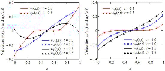
Figure 3. Comparison between $w_c(z,t),\hspace{0.17em}\hspace{0.17em}{w}_s(z,t)$ and $w_{fc}(z,t),\hspace{0.17em}\hspace{0.17em}{w}_{fs}(z,t)$ when $\alpha =1$ for $\omega =\pi /2,\hspace{0.17em}\hspace{0.17em}\mathrm{We}=2.5,\hspace{0.17em}\hspace{0.17em}\mathrm{Ha}=2,\hspace{0.17em}\hspace{0.17em}K=1.5$ and three values of t.

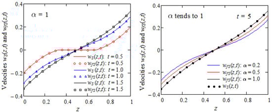
Figure 4. Comparison between the ordinary velocity $w_S(z,t)$ and fractional velocity $w_{fS}(z,t)$ for $\mathrm{We}=2.5,\hspace{0.17em}\hspace{0.17em}\mathrm{Ha}=2,\hspace{0.17em}\hspace{0.17em}K=1.5$, $\alpha =1$ and when $\alpha \to 1$.

The corresponding expressions for ${\eta }_{fc}(z,t)$, ${\eta }_{fs}(z,t)$, and ${\eta }_{fS}(z,t)$ and $R_{fc}(z,t)$, $R_{fs}(z,t)$, and $R_{fS}(z,t)$ are easily obtained using Equations (85) and (86) and the identity (A7) from Appendix A. Expressions of ${\eta }_{fS}(z,t)$ and $R_{fS}(z,t)$, for instance, are given by the following relations

$${\eta }_{fS}(z,t)=\frac{t^{\alpha -1}}{\mathrm{We}\hspace{0.17em}}{E}_{\alpha ,\alpha }\left(-\frac{1}{\mathrm{We}}{t}^{\alpha }\right)\ast \frac{\mathsf{\partial }{w}_{fS}(z,t)}{\mathsf{\partial }z},$$

(91)

$$R_{fS}(z,t)=-\frac{K{t}^{\alpha -1}}{\mathrm{We}\hspace{0.17em}}{E}_{\alpha ,\alpha }\left(-\frac{1}{\mathrm{We}}{t}^{\alpha }\right)\ast w_{fS}(z,t).$$

(92)

Figure 4 (when $\alpha \to 1)$ shows that the diagrams of the stating velocity $w_{fS}(z,t)$ tend to superpose over the profile of $w_S(z,t)$ when the fractional parameter $\alpha \to 1$.

Finally, it is worth pointing out the fact that the dimensionless volume fluxes $Q_c,\hspace{0.17em}\hspace{0.17em}{Q}_s$$Q_S$ as well as $Q_{fc},\hspace{0.17em}\hspace{0.17em}{Q}_{fs}$$Q_{fS}$ across a plane normal to the flow direction and per unit width of this plane are zero. Indeed, by introducing the expressions of these entities into Equation (17) and evaluating the integral, one obtains the zero value. This result is not a surprise; it is in accordance with the graphical representations presented in Figure 3 and Figure 4, in which the profiles of the respective entities are symmetric with respect to the median plane $z=0$, and their values in the two parts of the flow domain have contrary signs.

4.2. Steady Solutions for Some Non-Steady Motions of FECIMFs

In Section 3, it was proved that some unsteady motions of ECIMFs become steady in time. Let us now show that, if the functions $h_{\mathcal{l}}(\cdot )$ and $h_u(\cdot )$ have finite limits at infinity, i.e.,

$$\underset{t\to \infty }{\lim }{h}_{\mathcal{l}}(t)=h_{\mathcal{l}}^0<\infty \mathrm{and} \underset{t\to \infty }{\lim }{h}_u(t)=h_u^0<\infty ,$$

(93)

then the corresponding starting solution $w_f(z,t)$ given by Equation (84) becomes steady in time. To do this, let us denote, using $w_{fp}(z)$, the limit of $w_f(z,t)$ when t tends to infinity if it exists and use the identities (A8) and (A9) from Appendix A. Consequently, multiplying Equation (72) by s, taking the limit of result when $s\to 0$ and using the relations (93), one finds that

$$\begin{array}{l}{w}_{fp}(z)=\underset{t\to \infty }{\lim }{w}_f(z,t)=\underset{s\to 0}{\lim }[s{\overline{w}}_f(z,s)]=\frac{1}{2}\left(z^2-\frac{1}{3}\right)h_u^0-\left(\frac{1}{2}{z}^2-z+\frac{1}{3}\right)h_{\mathcal{l}}^0\\ +\frac{h_u^0-h_{\mathcal{l}}^0}{{\mathrm{Ha}}^2+K}+2{\displaystyle \sum _{n=1}^{\infty }\frac{({\mathrm{Ha}}^2+K)[h_{\mathcal{l}}^0+{(-1)}^{n+1}{h}_u^0]}{{\lambda }_n^2({\lambda }_n^2+{\mathrm{Ha}}^2+K)}}\cos ({\lambda }_{n}z);\hspace{0.17em}\hspace{0.17em}\hspace{0.17em}\hspace{0.17em}0<z<1,\end{array}$$

(94)

Here, by using the identity (A8) from Appendix A $a=(h_u^0-h_{\mathcal{l}}^0)/2$ and $b=h_{\mathcal{l}}^0$, it is not difficult to show that

$$2{\displaystyle \sum _{n=1}^{\infty }\frac{h_{\mathcal{l}}^0+{(-1)}^{n+1}{h}_u^0}{{\lambda }_n^2}}\cos ({\lambda }_{n}z)=-\frac{1}{2}\left(z^2-\frac{1}{3}\right)h_u^0+\left(\frac{1}{2}{z}^2-z+\frac{1}{3}\right)h_{\mathcal{l}}^0;\hspace{0.17em}\hspace{0.17em}\hspace{0.17em}\hspace{0.17em}0<z<1.$$

(95)

Using relations (94) and (95), one obtains the expression of the steady solution, namely,

$$w_{fp}(z)=\frac{h_u^0-h_{\mathcal{l}}^0}{{\mathrm{Ha}}^2+K}-2{\displaystyle \sum _{n=1}^{\infty }\frac{h_{\mathcal{l}}^0+{(-1)}^{n+1}{h}_u^0}{{\lambda }_n^2+{\mathrm{Ha}}^2+K}}\cos ({\lambda }_{n}z);\hspace{0.17em}\hspace{0.17em}\hspace{0.17em}\hspace{0.17em}0<z<1.$$

(96)

In the particular case when $h_{\mathcal{l}}(t)=h_u(t)=h(t)$ the above relation becomes

$$w_{fSp}(z)=-4h{\displaystyle \sum _{n=1}^{\infty }\frac{\cos ({\lambda }_{2n-1}z)}{{\lambda }_{2n-1}^2+{\mathrm{Ha}}^2+K}};\hspace{0.17em}\hspace{0.17em}\hspace{0.17em}\hspace{0.17em}0<z<1,$$

(97)

where $h=\underset{t\to \infty }{\lim }h(t)$. In the case when $h(t)=H(t)$ and $h=1$, the steady solution $w_{fSp}(z)$ from Equation (97) becomes equal to $w_{Sp}(z)$ from Equation (59). Consequently, the steady solutions $w_{Sp}(z)$ and $w_{fSp}(z)$ and the corresponding MHD motions of ECIMFs and FECIMFs, respectively, through a porous medium between infinite horizontal parallel plates, are identical.

5. Some Numerical Results and Conclusions

Exact general solutions are first time obtained for MHD unsteady motions of ECIMFs when differential expressions of the non-trivial shear stress are prescribed on the boundary. Such boundary conditions, as specified by Renardy [24,25], are specific for motions of rate-type fluids. The motions that have been considered here take place in a porous medium between two infinite horizontal parallel plates. Closed-form expressions are determined for the dimensionless starting velocity and the corresponding shear stress and Darcy’s resistance for both ordinary and fractional fluids. For illustration, as well as for the validation of the results, three particular cases are considered, and the starting velocities corresponding to these motions of ordinary fluids are presented as sums of their steady and transient components. For validation, the steady components of velocities are presented in different forms, the equivalence of which is graphically proved in Figure 2. We would also like to emphasize the fact that exact solutions can be used to verify numerical methods that are developed to study more complex motion problems.

It is worth pointing out the fact that the three motions of ECIMFs become steady in time, and an important problem for experimental researchers is to know the time after which the steady state is touched. A similar problem could be discussed for the unsteady movements of FECIMFs. More exactly, one must verify whether these motions become steady or not. To do that, we showed that a large class of unsteady motions of FECIMFs becomes steady in time. More precisely, if the two functions $h_{\mathcal{l}}(\cdot )$ and $h_u(\cdot )$ that appear in the boundary conditions (16), (66), and (67) satisfy the conditions (93), the corresponding motions of FECIMFs become steady in time, and the expression of steady velocity $w_{fp}(z)$ is given by Equation (96). In addition, if $h_{\mathcal{l}}(t)=h_u(t)=H(t)$, the steady component $w_{fSp}(z)$$w_{fS}(z,t)$ given by Equation (97) becomes identical to $w_{Sp}(z)$ Equation (59).

Here, in order to bring to light some characteristics of the behaviour of the fluids in the discussion, Figure 5, Figure 6, Figure 7 and Figure 8 are prepared for fixed values of physical parameters and increasing values of z and t and the fractional parameter $\alpha$. The convergence of the starting velocity $w_{fS}(z,t)$ to its steady-state component $w_{fSp}(z)$ is shown in Figure 5 for $\mathrm{We}=2.5,\hspace{0.17em}\hspace{0.17em}\mathrm{Ha}=2,\hspace{0.17em}\hspace{0.17em}K=1.5$, $\alpha =0.7$ and 0.9, and increasing values of time t.

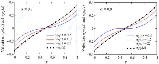
Figure 5. Convergence of the starting velocity $w_{fS}(z,t)$ to $w_{fSp}(z)$ for $\mathrm{We}=2.5,$ $\mathrm{Ha}=2,\hspace{0.17em}\hspace{0.17em}K=1.5,$ two values of $\alpha$ and increasing values of the time.

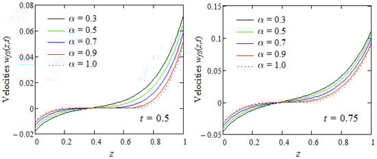
Figure 6. Profiles of starting velocity $w_{fS}(z,t)$ given by Equation (90) for $\mathrm{We}=2.5,$ $\mathrm{Ha}=2,\hspace{0.17em}\hspace{0.17em}K=1.5,$ increasing values of $\alpha$ and two values of the time t.

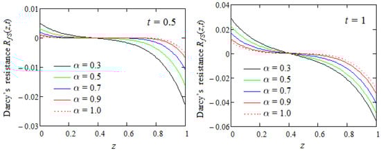
Figure 7. Profiles of Darcy’s resistance $R_{fS}(z,t)$ given by Equation (92) for $\mathrm{We}=2.5,\hspace{0.17em}\hspace{0.17em}\mathrm{Ha}=2,$ $K=1.5,$ two values of the time t and increasing values of the fractional parameter $\alpha$.

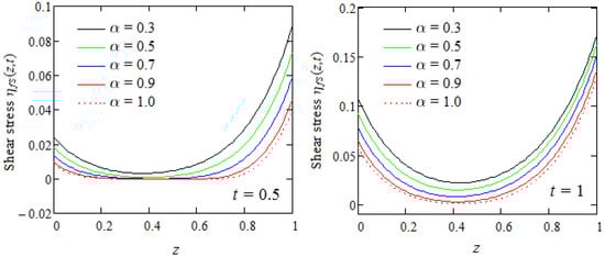
Figure 8. Profiles of shear stress ${\eta }_{fS}(z,t)$ given by Equation (91) for $\mathrm{We}=2.5,\hspace{0.17em}\hspace{0.17em}\mathrm{Ha}=2,\hspace{0.17em}\hspace{0.17em}K=1.5$, two values of the time t and increasing values of the fractional parameter $\alpha$.

The profiles of $w_{fS}(z,t)$ tend to superpose over the profile of $w_{fSp}(z)$ for increasing values of time t. They become almost identical at moment $t=80$ when $\alpha =0.7$ and $t=25$ for $\alpha =0.9$. Consequently, the need for time to reach the steady state diminishes for increasing values of $\alpha$. This means that the steady or permanent state is rather touched for motions of the fractional fluids in comparison to ordinary fluids.

Figure 6 presents profiles of the dimensionless starting velocity $w_{fS}(z,t)$ for increasing values of the fractional parameter $\alpha$ at two different times. In both cases, the fluid velocity is an increasing function with respect to the spatial variable z across the whole flow domain. However, contrary to the rule, a part of the fluid flows in one direction and the other part flows in the opposite direction. More exactly, there is a critical value $z_c$ (a little less than 0.4) of the spatial variable z that separates the two flow zones. In the first zone, adjacent to the lower plate, the fluid velocity is an increasing function $\alpha$.

An opposite situation appears in the other zone adjacent to the upper plate. Consequently, the ordinary fluids flow slower in comparison to the fractional fluids across the whole flow domain. In addition, as expected, fluid velocity increases over time.

Figure 7 presents the profiles of Darcy’s resistance $R_{fS}(z,t)$ with the same values as the physical parameters shown in Figure 6 and increasing values for the fractional parameter $\alpha$. As expected, the predictions of these figures are in correlation with those from Figure 6. For instance, the starting resistance $R_{fS}(z,t)$ is a decreasing function with regard to the fractional parameter $\alpha$ across the whole flow domain and its values, contrary to those of $w_{fS}(z,t)$, are positive in the inferior zone of the channel and negative in its upper part.

Last Figure 8 presents profiles of the dimensionless shear stress ${\eta }_{fS}(z,t)$ when $t=0.5$ and $t=1$ for increasing values of the fractional parameter $\alpha$.

In both cases, the shear stress is a decreasing function with respect to $\alpha$ across the entire flow domain. For each value $\alpha$, it diminishes from maximum values on the lower plate up to minimum values around the value $z=0.4$ of the spatial variable z and then increases on the rest of the flow domain. The shear stress ${\eta }_{fS}(z,t)$, unlike the fluid velocity $w_{fS}(z,t)$, which has opposite signs on the two zones of the flow domain, is positive everywhere.

The most important results that were obtained herein are as follows:

-

General solutions were established for some MHD unidirectional motions of ECIMFs and FECIMFs between infinite horizontal parallel plates incorporated into a porous medium when differential expressions of non-trivial shear stress were prescribed on the boundary.

-

The correctness of the obtained results was graphically proven for the fluid velocity both for motions of ordinary fluids and fractional fluids.

-

It was proven that a large class of unsteady motions of FECIMFs becomes steady in time.

-

A steady state corresponding to the motion due to a constant differential expression of shear stress on the boundary was obtained for ECIMFs rather than FECIMFs.

-

Some important characteristics concerning the behaviour of fractional Maxwell fluids were graphically brought to light and discussed.

-

It is worth mentioning that in such motions, contrary to the usual rule, the fluid flows in a direction on one part of the channel and in the opposite direction on the other part.

-

Volume fluxes across a plane normal to the flow direction per unit width of this plane are zero for the previously studied motions of both ECIMFs and FECIMFs.

References

- Ferry, J.D. Viscoelastic Properties of Polymers, 3rd ed.; John Wiley & Sons: New York, NY, USA, 1980. [Google Scholar]
- Maxwell, J.C. On the dynamical theory of gases. Philos. Trans. R. Soc. 1867, 157, 49–88. [Google Scholar] [CrossRef]
- Böhme, G. Stromungsmechanik Nicht-Newtonscher Fluide; Verlag B.G. Teubner: Stuttgart, Germany, 2000. [Google Scholar]
- Srivastava, P.N. Non-steady helical flow of a visco-elastic liquid. Arch. Mech. Stos. 1966, 18, 145–150. [Google Scholar]
- Wang, S.; Li, P.; Zhao, M. Analytical study of oscillatory flow of Maxwell fluid through a rectangular tube. Phys. Fluids 2019, 31, 063102. [Google Scholar] [CrossRef]
- Sun, X.; Wang, S.; Zhao, M. Oscillatory flow of Maxwell fluid in a tube of isosceles right triangular cross section. Phys. Fluids 2019, 31, 123101. [Google Scholar] [CrossRef]
- Hayat, T.; Fetecau, C.; Abbas, Z.; Ali, N. Flow of a Maxwell fluid between two side walls due to a suddenly moved plate. Nonlinear Anal. Real World Appl. 2008, 9, 2288–2295. [Google Scholar] [CrossRef]
- Palade, L.I.; Attane, P.; Huilgol, R.R.; Mena, B. Anomalous stability behaviour of a properly invariant constitutive equation which generalizes fractional derivative models. Int. J. Eng. Sci. 1999, 37, 315–329. [Google Scholar] [CrossRef]
- Rossikhin, Y.A.; Shitikova, M.V. A new method for solving dynamic problems of fractional derivative viscoelasticity. Int. J. Eng. Sci. 2001, 39, 149–176. [Google Scholar] [CrossRef]
- Makris, N. Theoretical and Experimental Investigation of Viscous Dampers in Applications of Seismic and Vibration Isolation. Ph.D. Thesis, State University of New York at Buffalo, Buffalo, NY, USA, 1991. [Google Scholar]
- Makris, N.; Constantinou, M.C. Fractional derivative model for viscous dampers. J. Struct. Eng. ASCE 1991, 117, 2708–2724. [Google Scholar] [CrossRef]
- Bagley, R.L. A theoretical basis for the application of fractional calculus to viscoelasticity. J. Rheol. 1983, 27, 201–210. [Google Scholar] [CrossRef]
- Friedrich, C. Relaxation and retardation functions of the Maxwell model with fractional derivatives. Rheol. Acta 1991, 30, 151–158. [Google Scholar] [CrossRef]
- Mainardi, F. Fractional relaxation-oscillation and fractional diffusion-wave phenomena. Chaos Solitons Fractals 1996, 7, 1461–1467. [Google Scholar] [CrossRef]
- Hristov, J. Response functions in linear viscoelastic constitutive equations and related fractional operators. Math. Model. Nat. Phenom. 2019, 14, 305. [Google Scholar] [CrossRef]
- Tan, W.C.; Xu, M.Y. Plane surface suddenly set in motion in a viscoelastic fluid with fractional Maxwell model. Acta Mech. Sin. 2002, 18, 342–349. [Google Scholar] [CrossRef]
- Tan, W.C.; Pan, W.; Xu, M.Y. A note on unsteady flows of a viscoelastic fluid with the fractional Maxwell model between two parallel plates. Int. J. Non Linear Mech. 2003, 38, 645–650. [Google Scholar] [CrossRef]
- Hayat, T.; Nadeem, S.; Asghar, S. Periodic unidirectional flows of viscoelastic fluid with fractional Maxwell model. Appl. Math. Comput. 2004, 151, 153–161. [Google Scholar] [CrossRef]
- Shaowei, W.; Mingyu, X. Exact solutions on unsteady Couette flow of generalized Maxwell fluid with fractional derivative. Acta Mech. 2006, 187, 103–112. [Google Scholar] [CrossRef]
- Qi, H.; Xu, M. Unsteady flow of a viscoelastic fluid with fractional Maxwell model in a channel. Mech. Res. Comm. 2007, 34, 210–212. [Google Scholar] [CrossRef]
- Corina, F.; Athar, M.; Fetecau, C. Unsteady flow of a generalized Maxwell fluid with fractional derivative due to a constantly accelerating plate. Comput. Math. Appl. 2009, 57, 596–603. [Google Scholar] [CrossRef]
- Ullah, H.; Lu, D.; Siddiqui, A.M.; Harood, T.; Maqbool, K. Hydrodynamical study of creeping Maxwell fluid flow through a porous slit with uniform reabsorption and wall slip. Mathematics 2020, 8, 1852. [Google Scholar] [CrossRef]
- Fetecau, C.; Ellahi, R.; Sait, S.M. Mathematical analysis of Maxwell fluid flow through a porous plate channel induced by a constantly accelerating or oscillating wall. Mathematics 2021, 9, 90. [Google Scholar] [CrossRef]
- Renardy, M. Inflow boundary conditions for steady flow of viscoelastic fluids with differential constitutive laws. Rocky Mt. J. Math. 1988, 18, 445–453. [Google Scholar] [CrossRef]
- Renardy, M. An alternative approach to inflow boundary conditions for Maxwell fluids in three space dimensions. J. Non-Newtonian Fluid Mech. 1990, 36, 419–425. [Google Scholar] [CrossRef]
- Fetecau, C.; Rauf, A.; Qureshi, T.M.; Vieru, D. Steady-state solutions for MHD motions of Burgers’ fluids through porous media with differential expressions of shear on boundary and applications. Mathematics 2022, 10, 4228. [Google Scholar] [CrossRef]
- Cramer, K.R.; Pai, S.I. Magnetofluid Dynamics for Engineers and Applied Physicists; McGraw-Hill: New York, NY, USA, 1973. [Google Scholar]
- Khan, M.; Malik, R.; Anjum, A. Exact solutions of MHD second Stokes flow of generalized Burgers fluid. App. Math. Mech. Engl. 2015, 36, 211–224. [Google Scholar] [CrossRef]
- Sneddon, I.N. Fourier Transforms; McGraw-Hill: New York, NY, USA, 1951. [Google Scholar]
Disclaimer/Publisher’s Note: The statements, opinions and data contained in all publications are solely those of the individual author(s) and contributor(s) and not of MDPI and/or the editor(s). MDPI and/or the editor(s) disclaim responsibility for any injury to people or property resulting from any ideas, methods, instructions or products referred to in the content. |
© 2024 by the authors. Licensee MDPI, Basel, Switzerland. This article is an open access article distributed under the terms and conditions of the Creative Commons Attribution (CC BY) license (https://creativecommons.org/licenses/by/4.0/).