Abstract
Spatial regression models are widely available across several disciplines, such as functional magnetic resonance imaging analysis, econometrics, and house price analysis. In nature, sparsity occurs when a limited number of factors strongly impact overall variation. Sparse covariance structures are common in spatial regression models. The spatial error model is a significant spatial regression model that focuses on the geographical dependence present in the error terms rather than the response variable. This study proposes an effective approach using the pretest and shrinkage ridge estimators for estimating the vector of regression coefficients in the spatial error mode, considering insignificant coefficients and multicollinearity among regressors. The study compares the performance of the proposed estimators with the maximum likelihood estimator and assesses their efficacy using real-world data and bootstrapping techniques for comparison purposes.
Keywords:
spatial error model; asymptotic performance; bootstrapping; pretest; ridge estimator; shrinkage MSC:
62J07; 62H12; 91B72
1. Introduction
Data collected over a geographic region may be generally more comparable than data from far away. This phenomenon can be modeled using a covariance structure in conventional statistical models. Spatial regression models, incorporating various spatial dependencies, are increasingly being used in geology, epidemiology, disease monitoring, urban planning, and econometrics.
Time series autoregressive models represent data at time t as linear combinations of the most recent observations. Similarly, in the spatial framework, these models display data from a specific location based on neighboring locations. Data are typically collected from a geographical location known as a site, and proximity is defined by a distance metric.
One of the most used autoregressive models is the spatial error(SE) model, in which a linear regression with a spatially lagged autoregressive error component is used to model the spatial response variable’s mean. Ref. [1] investigated the quantile regression estimation for the SE model with potentially variable coefficients. The authors established the proposed estimators’ asymptotic properties. Ref. [2] applied the SE model to examine the existence of spatial clustering and correlation between neighboring counties for the data from Egypt’s 2006 census. Ref. [3] used the SE model to evaluate the social disorganization theory. Ref. [4] used the combined application of the SE model and spatial lag model based on cross-sectional data from 20 districts in Chengdu. The authors found that the haze had a negative impact on both the selling and rental prices of houses. Ref. [5] proposed a robust estimation method based on SE models, demonstrating reduced bias, a more stable empirical influence function, and robustness to outliers through simulation. More information about the spatial autoregressive models can be found in [6,7,8], among others.
In frequentist statistics, sample information is used to establish inferences about unknown parameters, while Bayesian statistics combines sample information with uncertain prior information (UPI) to draw conclusions. Subjective UPI may not always be available. However, model selection procedures like Akaike’s information criterion (AIC), Bayesian information criterion (BIC), or model selection techniques can still provide UPI.
An initial trial to estimate the regression parameters using sample information and UPI is called a pretest estimation. The pretest estimator selects significant regression coefficients and chooses between the full model estimator or the revised model estimator, which contains fewer coefficients based on a binary weight. A new modification of the pretest estimator, known as the shrinkage estimator, uses smooth weights between full and sub-model estimators to adjust regression coefficient estimates toward a target value impacted by UPI. Nevertheless, the modified shrinkage estimator suffers sometimes from an over-shrinkage phenomenon. Later, an improved version of this estimator, known as positive shrinkage, controls the over-shrinkage issue.
The concept of using pretest and shrinkage estimating methodologies has received considerable attention from many researchers; for example, ref. [9] introduced an efficient estimation using pretest and shrinkage methods to estimate the regression coefficient vector of the marginal model in the case of multinomial responses. Ref. [10] developed different shrinkage and penalty estimation strategies for the negative binomial regression model when over-fitting and uncertain information exists about the subspace. Ref. [11] proposed shrinkage estimation for the parameter vector of the linear regression model with heteroscedastic errors, and extended their study to the high-dimensional heteroscedastic regression model.
Multicollinearity is a major issue when fitting a multiple linear regression model using the ordinary least squares (OLS) method, which arises when some regressor variables are correlated, especially when the correlation between any two is high. There are several techniques discussed in the literature to reduce the risk of this issue. Ref. [12] introduced the concept of ridge regression as a solution to nonorthogonal problems. They showed that the estimator improves the mean square error of estimation. Ref. [13] introduced a new biased estimator and demonstrated, both theoretically and numerically, the improvements of the new one. Ref. [14] proposed a new version of the Liu estimator for the vector of parameters in a linear regression model based on some prior information.
Using the idea of shrinkage, ref. [15] introduced an improved form of the Liu-type estimator. Analytical and numerical results were used to demonstrate the proposed method’s superiority. Ref. [16] suggested the use of the ridge estimator as a suitable approach for handling high-dimensional multicollinearity data. Recently, ref. [17] proposed a novel pretest and shrinkage estimate technique, known as the Liu-type approach, developed for the conditional autoregressive model.
In this article, we propose the ridge-type pretest and shrinkage estimation strategy for the regression coefficients vector in the SE model when some prior information is available about the irrelevant coefficients. We will partition the vector as , where is a vector that contains the coefficients of the main effect, and is a vector of irrelevant coefficients, with . Mainly, we focus on estimating the vector when the UPI indicates that is ineffective, which can be achieved by testing a statistical hypothesis of the form . In some instances, the estimator of the full model may exhibit considerable variability and provide challenges in terms of interpretation. Conversely, the estimator of the sub-model may yield a significantly biased and under-fitted estimate. To tackle this matter, we took into account the pretest, shrinkage, and positive shrinkage ridge estimators for the vector .
In accordance with our goal, this paper is organized as follows. Section 2 offers an overview of the SE model. A discussion about the maximum likelihood estimators for the parameters of the SE model is presented in Section 3. In Section 4, we propose the pretest and shrinkage ridge estimators. Asymptotic analysis of the proposed estimators and some theoretical results are presented in Section 5. The estimators are compared numerically using simulated and real data examples in Section 6. Some concluding remarks are presented in Section 7. An appendix containing some proofs is presented at the end of this manuscript.
2. Spatial Error Model
Let represent a set of spatial sites (frequently known as locations, regions, etc.). Set forms what is commonly referred to as a lattice, and the set of nearby sites for , denoted by , is defined as follows: , . A neighborhood structure can be determined using a predefined adjacency metric. In regular lattices, if two sites just share edges, they are rook-based neighbors; if they also share borders and/or corners, they are queen-based neighbors.
Let be a vector of observations collected at sites , be the matrix of covariates, and be the vector of unknown regression parameters, known as the large-scale effect. Following Cressie and Wikle [7], the SE model models the response at the site as follows:
where is the noise vector that has a Gaussian distribution with a mean of and the covariance matrix . Parameters are used to model the spatial dependencies among the errors , with . Let , and assume that is invertible, where is the identity matrix, then by ignoring the spatial indices, the SE in (1) can be rewritten in matrix form, as follows:
Nature exhibits sparsity in many situations, which means that a small number of factors can account for the majority of the observed variability. In the context of regression analysis, sparsity means a few numbers of the coefficients are significantly different from zero, while the bulk of the coefficients are insignificant and remain zero. Sparsity is frequently used in spatial regression models to imply covariance structures that are easier to compute. Consequently, by setting , and , where is the variance component, is the spatial dependence parameter, and is the weight or proximity-known matrix with a main diagonal of zeros, and off-diagonal entices if the location j is a neighbor to location i; otherwise, , the preceding model yields a straightforward and frequently used version. Usually, the weight matrix is normalized as . So, the SE regression model can be rewritten as follows:
3. Maximum Likelihood Estimation
Let ; the maximum likelihood estimator (MLE) of may be acquired by the use of a two-step profile-likelihood method; see [6]. At first, we fix and find the MLEs of as a function of , which are given as follows:
Then, we plug and into the log-likelihood and obtain the MLE of by maximizing the profile’s log-likelihood function. Finally, the MLEs of and are computed by replacing with in Equations (6) and (7), respectively. Ref. [18] proved that is a consistent estimator of , and asymptotically has normal distribution. This finding makes it simple to demonstrate that is asymptotically normal and consistent. The significance of regression coefficients can often be determined subjectively or through certain model selection techniques in various situations. As a result of this information, the regression coefficient vector is divided into two sub-vectors, as , where is a vector of important coefficients and is a vector of unimportant coefficients with . Similarly, the matrix of covariates is also partitioned as , where and consist of the first and the last columns of the design matrix of dimensions and , respectively. Consequently, the SE full model in (3) can be rewritten as follows:
For the full model in (8), we can obtain the MLEs of using the same technique employed in model (4); see [19]. The MLEs are as follows:
and has an identical formula as by exchanging indices 1 and 2 in the above two equations. The full model estimation may be prone to significant variability and may be difficult to interpret. Our primary goal is to estimate the value of when the set of regressors included in the partitioned matrix does not sufficiently explain the variability in the response variable, which can be achieved by formulating a linear hypothesis as follows:
Assuming the null hypothesis in (10) is true, the updated model based on this assumption of the model, given (8), becomes
We will refer to the model in (11) as the restricted SE model. Let be the MLE of of the model in (11), then
Obviously, will have better performance than if the null hypothesis in (10) is true, while the opposite occurs when begins to move away from the null space. Yet, the restricted strategy method can provide the under-fitted and highly biased model. One goal of this research is to overcome the problem of significant bias in spatial error models when multicollinearity is present among the regressors. To address this issue, we suggest using a ridge-type estimate approach for both the full and sub-models to enhance these estimators by incorporating pretest and shrinkage estimating approaches, to reduce biases and improve the overall accuracy of the estimators. To dominate the large bias, we propose the ridge-type estimation strategy of the full and reduced models and then improve the two estimators using the pretest and shrinkage estimation idea.
4. Materials and Methods: Developing Pretest and Shrinkage Ridge Estimation Strategies
In this section, we propose a set of estimators for the SE model parameter vector in (11). Following [12], the ridge estimator of for the model given in (4) is defined as
where is known as the ridge parameter. Clearly, when , the ridge estimator reduces to the MLE of , but if , the ridge estimator .
4.1. Full and Reduced Model Ridge Estimators
The unrestricted full model ridge estimator of , denoted by , is defined as follows:
where represents the ridge parameter for the unretracted full model estimator, denoted as . Assuming the null hypothesis in (10) is true, the restricted ridge estimator of for the model in (11), denoted by , is given by
where is the ridge parameter for restricted model estimator . When the null hypothesis in (10) is accurate or almost accurate (i.e., when is close to zero), is generally a more effective estimator than . Nevertheless, as deviates from the zero space, becomes inefficient compared with the unrestricted estimator . In addition to the gain obtained by employing the ridge estimation idea to the MLE of , we also aim to find estimators that are functions of and , and intend to lessen the dangers connected with any of these two estimators over the majority of the parameter space. The pretest and shrinkage estimators, which will be built in the following subsection, can help with this.
4.2. Pretest, Shrinkage, and Positive Shrinkage Ridge Estimators
In line with testing the null hypothesis in (10), the pretest estimator selects either the full model estimator if is rejected or the restricted ridge estimator if not. An appropriate test statistic to test the hypothesis in (10) is
where is defined in a similar manner, as , , and , which is a consistent estimator of , and statistic asymptotically follows a chi-square distribution with degrees of freedom under the null hypothesis. Hence, the pretest estimator, denoted by , is given by
where is an indicator function, and is the upper th quantile of the chi-square distribution with degrees of freedom. The pretest estimator depends on the level of the significance , and selects if the null hypothesis is rejected, and otherwise, based on binary weights. These drawbacks can be improved using smoother weights of the two estimators and instead, which is known as the shrinkage estimator. It is denoted by, , and given by
The shrinkage estimator may experience an over-shrinkage in which negative coordinates may be produced whenever . The positive shrinkage estimator, a modified version of , resolves this issue. It is denoted by , and given by
where It is easy to see that all the pronounced shrinkage estimators satisfy the following general form
Simply, for , , and , the corresponding functions are given by , , and , respectively.
5. Asymptotic Analysis
In this section, we will study the asymptotic performances of all estimators based on their asymptotic quadratic risks. Our goal is to investigate the behavior of the set of estimators near the null space, so we consider a sequence of local alternatives given by
Obviously, when , the local alternatives in (20) may be simplified to the null hypothesis given in (10). Assuming that represents the cumulative distribution function of any estimator of , say , then: . Thus, for any positive definite matrix , the weighted quadratic loss function is defined as
where is the trace of the matrix . Define , then if , where denotes the convergence in distribution, then the asymptotic (distributional) quadratic risk (ADQR) of , denoted by , is given by
The asymptotic (distributional) bias (ADB) of can be obtained via
To derive asymptotic distributional properties, in addition to the first four assumptions of [18], we set the following regularity conditions:
- (A1)
- , as , where is the ith row of .
- (A2)
- Let . Then, , where is the positive definite matrix.
- (A3)
- LetThen, , where for .
In the following, we refer to the above assumptions as the “named regularity condition (NRC)”.
The primary tool to derive expressions of the asymptotic quadratic risks for the proposed estimators is to find the asymptotic distribution of the unrestricted full model ridge estimator and the restricted ridge estimator . To this end, we make use of the following lemma. The proof is provided in Appendix A.
Lemma 1.
Assume the NRC. If , then
where denotes convergence in distribution. Indeed, Lemma 1 enables us to provide some asymptotic distributional results about the estimators and , as presented in the following theorem, which are easy to prove.
Theorem 1.
Let , , and . Assume the local alternatives in (20) and NRC. Then, as , we have
- 1.
- 2.
- 3.
- 4.
- 5.
- 6.
- E
- 7.
- , where is the cumulative distribution function of a non-central chi-square distribution with q degrees of freedom and the Δ non-centrality parameter.Where , , .
With Lemma 1 in hand, it is pretty straightforward to reach the asymptotic distributional properties of the shrinkage estimators. Through the subsequent theorems, we will provide the asymptotic bias and weighted quadratic risk functions.
Theorem 2.
Under the assumptions of Lemma 1, the asymptotic distributional bias of the shrinkage estimators are given by
- 1.
- 2.
- 3.
- where
For the proof, refer to Appendix A.
The following results reveal the expressions for the ADQR of the proposed shrinkage estimators.
Theorem 3.
Under the assumptions of Lemma 1, the asymptotic distributional quadratic risks of the shrinkage estimators are given by
- 1.
- 2.
- 3.
where is a positive definite weight matrix,
For the proof, refer to Appendix A.
6. Numerical Analysis
To demonstrate our theoretical findings, we first use Monte Carlo simulation experiments and then apply the set of proposed estimators to a real dataset. The Monte Carlo simulation is used to investigate the performance of the ridge-type set of estimators in comparison to the MLE given in (9) via the simulated mean square error of each estimator.
6.1. Simulation Experiments
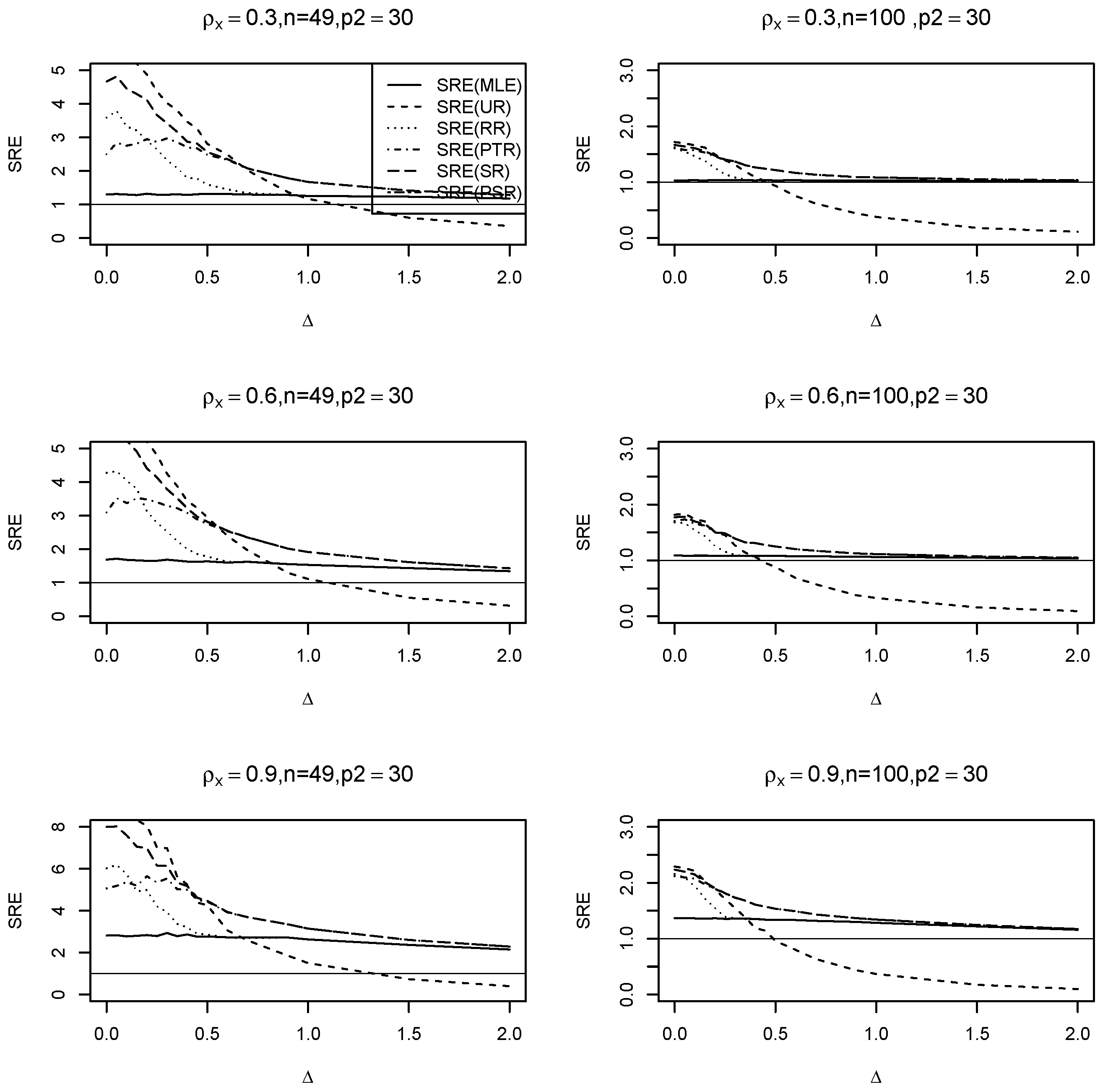
In this section, we compare the set of ridge-type estimators with respect to the MLE using Monte Carlo simulation experiments based on their simulated mean squared errors. In each of these experiments, we consider square lattices using with the corresponding sample sizes of , respectively. To show the performance of the proposed estimators when multicollinearity exists, we generate the design matrix from the multivariate normal distribution with a mean of , and a variance-covariance matrix with a first-order autoregressive structure, in which and apply it to , while the error term is generated from another multivariate normal with a mean of and an SE variance matrix with . We set . For the weight matrix , a queen-based contiguity neighborhood was used. The set of values for is . We partitioned the vector of coefficients as , where is a vector of ones, and , is a zero vector of dimension , and , where is the Euclidean norm of , and represents the non-centrality parameter. The range of values for is set to be from 0 to 2. Then we fit the model in (8) using the spautolm function within the R-package spdep [20], obtain the values of all estimators considered in our study, and compute the simulated mean square error (SMSE) of each estimator as . The simulated relative efficiency (SRE) of any estimator, say , with respect to the MLE , is calculated as follows:
where is any of the estimators . It is evident that when the is greater than one, it signifies that this estimate outperforms the MLE of the full model, and vice versa. We run the simulation for , and use to test the hypothesis in (20). No statistically significant change is seen while altering the spatial dependency parameter. Therefore, we simply exhibit the graphs for . Figure A1, Figure A2 and Figure A3 in Appendix A show the results of the SRE against various values of . The findings support the following conclusions:
- (i)
- Across all values, the ridge-type full model estimator consistently outperforms the traditional MLE estimator. Furthermore, as increases, so does its efficiency for fixed values of and . Additionally, when the multicollinearity among the explanatory variables in the design matrix becomes stronger, efficiency increases as expected.
- (ii)
- The ridge-type sub-model estimator outperforms all other estimators when . Since the null hypothesis is correct, it is expected. However, once begins to depart from the null space, the estimator’s SRE drops precipitously and approaches zero, making it less effective than the other estimators.
- (iii)
- The SRE values grow while holding other parameters constant, as the correlation coefficient increases among the explanatory factors.
- (iv)
- As the number of zero coefficients increase =, all SRE estimators also increase.
- (v)
- The ridge-type positive shrinkage estimator uniformly prevails over the competing estimators.
6.2. Data Example
In 1970, ref. [21] examined the use of housing market data for census tracts in the Boston Statistical Metropolitan Area. The authors’ major objective was to establish a relationship between a set of (15) variables and the median cost of owner-occupied residences in Boston. Ref. [22] offered a corrected version of the dataset along with new spatial data. The dataset is accessible through the R-Package spdep version 1.3-1. There are 506 observations in the data, each of which relates to a single census tract. The variables in the data include the tract identification number (TRACT), median owner-occupied housing prices in US dollars (MEDV), corrected median owner-occupied housing prices in US dollars (CMEDV), percentages of residential land zoned for lots larger than 2500 square feet per town (constant for all Boston tracts) (ZN), percentages of non-retail business areas per town (INDUS), average room sizes per home (RM), the percentage of owner-occupied homes built before 1940 (AGE), a dummy variable with two levels, which is 1 if the tract borders the Charles River and 0 otherwise (CHAS), the crime rate per capita (CRIM), the weighted distance to main employment centers (DIS), nitrogen oxide concentration (parts per 10 million) per town (NOX), an accessibility index to radial highway per town (constant for all Boston tracts) (RAD), property tax rate per town ($10,000) (constant for all Boston tracts) (TAX), percentage of the lower-class population (LSTAT), pupil–teacher ratios per town (constant for all Boston tracts) (PTRATIO), and the variable , where b is the proportion of blacks (B). Ref. [23] added the location of each tract in latitude (LAT), and longitude (LON) variables. Assuming an SE model, we can predict the response variable log(CMEDV) using all available variables, which will be referred to as the full SE model. For these data, a variety of selection techniques were used to determine the sub-model. One sub-model that was used by [19] is the model obtained by the adaptive LASSO algorithm, which will be referred to as our SE sub-model. The two models are summarized in Table 1.

Table 1.
Full and sub-model.
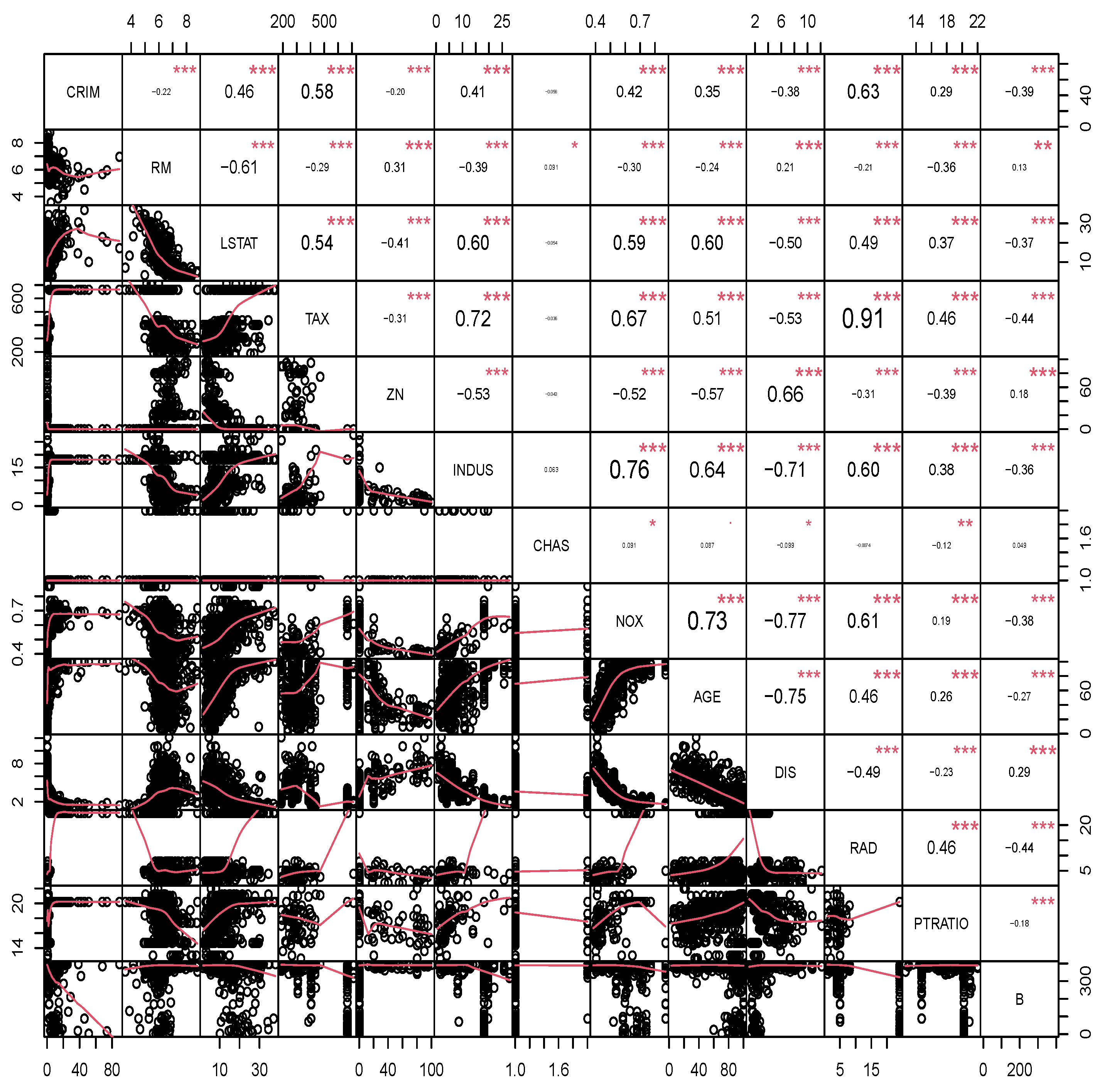
Figure 1 displays a colored plot of the correlation coefficients for each variable. The notation (***) indicates high significance with a p-value of less than 0.001. The notation (**) indicates significance at a 1% level, while (*) indicates significance at a 5% level. If none of these symbols are present, it signifies that the correlation coefficient between the two variables is not statistically significant. The CMEDV and a few other factors have a strong linear relationship, as seen in the plot. This plot is useful for examining the strength of linearity between the original response CMEDV and any other variable if it exists. The selected variables by the adaptive LASSO algorithm appear to have strong, medium, and weak relationships with the response variable. Moreover, some variables exhibit collinearity; this issue will show how ridge-type estimators show high performance compared to MLE estimators.
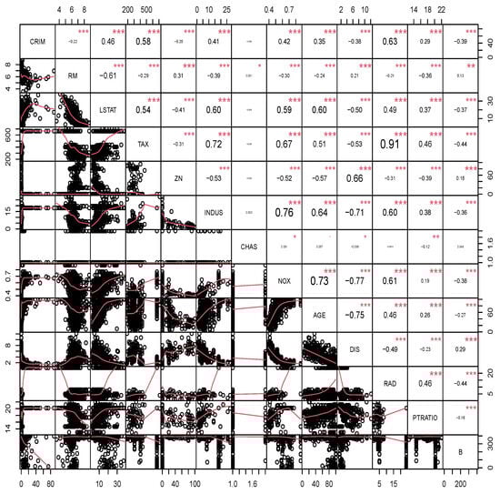
Figure 1.
Correlation matrix for the Boston housing data.
Table 2 presents the estimated ridge-type values of the proposed estimators.
Table 2.
Estimated values.
To assess the effectiveness of the suggested estimators, we will use two different methods, aiming to provide a reliable and valid evaluation of our results. The first method employs the bootstrapping methodology, whereas the second one involves validation using out-of-sample data.
The bootstrapping technique suggested by [24], computes the mean squared prediction error (MSPE) for any estimator as follows:
- Fit the SE full and sub-models as they appear in Table 1 using the spautolm function and obtain the MLEs of , , the spatial dependence parameter , and the covariance matrix .
- As the columns of matrices and are not orthogonal, and the sample size is large, we follow [25] to estimate the tuning ridge parameters for the two estimators, and , which are, respectively, given by, and .
- Use the Cholesky decomposition method to express the matrix in a decomposed form as , where is an lower triangular matrix.
- Let , where ; we define the centered residual as , and then select with the replacement a sample of size to obtain .
- Calculate the bootstrapping response value as , and then use it to fit the full and sub-models and obtain bootstrapping estimated values of all estimators.
- Calculate the predicted value of the response variable using each estimator as follows: , where represents any of the estimators in the set .
- For the bootstrapping sample, we calculate the square root of the mean square prediction error (MSPE) aswhere B is the number of bootstrapping samples.
- Calculate the relative efficiency (RE) of any estimator with respect to the MLE as follows:where is any of the ridge-type proposed estimators. We apply the bootstrapping technique times.
Table 3 summarizes the results of the relative efficiencies, where a relative efficiency value exceeding one indicates the superior performance of the estimator in the denominator.
Table 3.
RE of the proposed estimators.
The second approach is based on out-of-sample data. In general, when using out-of-sample data for non-spatial regression models, it is assumed that the errors are independent. However, the errors in the SE regression model are not independent. Nonetheless, by employing a transformation, we may overcome this challenge. We suggest modifying the SE model to ensure the errors are independent while keeping and constant. A related transformation technique in spatial models can be found in [6]. Note that the covariance matrix is positive definite, so can be rewritten as , where is an upper triangular matrix with positive entries on the diagonal; see ([26], p. 338). By multiplying the model in (4) by , we obtain
where , , and , with . Practically, we obtain the MLEs of , and , and use these estimates to find the estimated matrix . The steps of using out-of-sample data are as follows:
- Create a data frame containing the columns of and .
- Divide the data frame into training and testing subsets. The testing data subset is known as the out-of-sample dataset.
- Using the training dataset, we follow the same procedure discussed in Section 3. That is, we divide the training data into two subsets, as , fit the full and sub-models, and obtain the array of estimators, which are denoted by , , , , , .
- Divide the testing data into two subsets, as , and calculate the predicted response values as follows:where is any of the estimators obtained in step (2).
- Compute the average of the MSPE using Equation (24), replacing with , and by .
We divide the dataset into for the taring set and for the testing set, respectively; we repeat steps (2–5) 2000 times, and then obtain the relative efficiency as in Equation (25). Table 4 shows the relative efficiency results based on out-of-sample data.
Table 4.
The RE of the proposed estimators using out-of-sample data.
Table 3 and Table 4 illustrate the better performance of the sub-model ridge-type estimator compared to all other estimators. It is then followed by the pretest estimator , demonstrating the correctness of the sub-model that was selected. Also, the ridge-positive shrinkage estimator performs better than the shrinkage one. Furthermore, all ridge-type estimators outperformed the MLE of .
7. Conclusions
This paper discusses the pretest, shrinkage, and positive shrinkage ridge-type estimators of the parameter vector for the SE model when there is a previous suspicion that certain coefficients are insignificant, and multicollinearity exists between two or more regressor variables. To obtain the proposed set of estimators for the main effect vector of coefficients , we test the hypothesis . The proposed estimators were compared analytically via their asymptotic distributional quadratic risks, and numerically through simulation experiments and a real data example.
Our results showed that there is no significant effect of the spatial dependence parameters , while the performance of the ridge estimators increases as the correlation among the regressor variables increases. Moreover, the performance of the ridge estimators is always better than the MLE. In addition, the estimator dominates all estimators under the null hypothesis , or when near the null space, and delivers higher efficiency than the other estimators. However, the proposed positive shrinkage ridge estimators perform better than the MLE in all seniors. Further, we apply the set of estimators to a real data example, and use bootstrapping and validation based on out-of-sample data techniques to evaluate their performance based on the relative efficacy of the square root of the mean squared prediction error.
The ridge-type pretest and shrinkage estimators significantly reduced the MSPE. These estimators handled spatial error models well by collecting and minimizing prediction variation. The lower MSPE shows that the proposed estimation strategy makes more accurate and trustworthy forecasts than MLE. This suggests that adding these estimators to the model improves predicted accuracy and model performance. This part of the residual analysis shows that ridge-type estimators are effective at addressing prediction errors in spatial error modeling.
The idea of a ridge-type pretest and shrinkage estimation strategy applies to a wide range of spatial regression models. Regarding continuous data, the method can be used for different models, such as the conditional autoregressive model, simultaneous autoregressive model, and spatial autoregressive moving average model. For discrete spatial data types, it can be applied to generalized linear models with a conditional autoregressive covariance structure, auto-logistic models for binary data, and auto-Poisson and negative binomial models for count data, among others. Lee, L. F [27] considered the estimation of the spatial model, which includes a spatial lag of the dependent variable and spatially autoregressive disturbances and provides the most effective spatial two-stage least squares (2SLS) estimator, which are instrumental variable estimators and optimal in the asymptotic sense. Such a method may be used and benefit from the pretest and shrinkage estimation strategy to improve the estimators of several spatial regression models. Liu and Yang [28] discussed the impact of spatial dependence on the convergence rate of quasi-maximum likelihood (QML) estimators and guided how to rectify the finite sample bias in the spatial error dependence model. Based on our findings, it is expected that employing the ridge-type pretest and shrinkage estimation for the spatial dependence model will be a beneficial addition, and provide better results in terms of the estimators’ biases.
Author Contributions
M.A.-M. initiated the research, designed the study, proposed estimators, established a methodology, did the numerical studies, including the simulation and the data example, analyzed findings, wrote a manuscript, underwent critical revision, and revised the final version. M.A. meticulously stages the research from design to final approval, including methodology, especially the theory, and the writing of the original manuscript, reviewing and editing, ensuring accuracy, clarity, and coherence of findings through an iterative process. All authors have read and agreed to the published version of the manuscript.
Funding
This research received no external funding.
Data Availability Statement
The dataset is accessible through the R-Package “spdep”.
Acknowledgments
We express our heartfelt gratitude to the four anonymous reviewers for their valuable feedback, which prompted us to include several details in the work and enhance its presentation.
Conflicts of Interest
The authors declare no conflict of interest.
Appendix A. Proofs of the Main Results
Proof of Lemma 1.
For the proof, we follow the approach of Yuzbasi et al. [29], with a slight modification. Let and define
where . Following [30],
with finite-dimensional convergence holding trivially. Also
Thus with the finite-dimensional convergence holding trivially. Since is convex and has a unique minimum, it follows that
It concludes
□
Proof of Theorem 2.
Because all of the pronounced estimators are special cases , we give the bias of this estimator here. Then the proof follows by applying relevant function in each estimator. Hence, we have
Using part one of Lemma 1, . Further using part three of Lemma 1 along with Theorem 1 in Appendix B of [31], we have
Therefore, the asymptotic bias of the general shrinkage estimator is given by
The proof is complete considering the expressions for given in Table A1. □
Table A1.
Expressions for the corresponding functions in the proposed shrinkage estimators.
Table A1.
Expressions for the corresponding functions in the proposed shrinkage estimators.
| Shrinkage Estimator | Function | |
|---|---|---|
Proof of Theorem 3.
Similar to the proof of Theorem 2, we provide the ADQR of the shrinkage estimator here. Then the proof follows by applying relevant function in each estimator. Hence, we have
From Lemma 1, we have
From Lemma 1
Using double expectation, parts three and six of Lemma 1, and Theorems 1 & 3 in Appendix B of [31], we have
Thus, it yields
In a similar manner, we have
Gathering all required expressions, we finally have
The proof is complete using Table A1. □
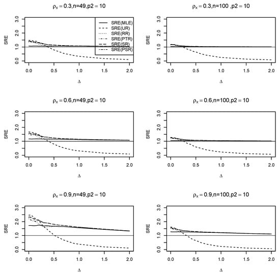
Figure A1.
SRE of the suggested estimators with respect to the MLE () for , , , and .
Figure A1.
SRE of the suggested estimators with respect to the MLE () for , , , and .

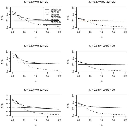
Figure A2.
SRE of the suggested estimators with respect to the MLE () for , , , and .
Figure A2.
SRE of the suggested estimators with respect to the MLE () for , , , and .
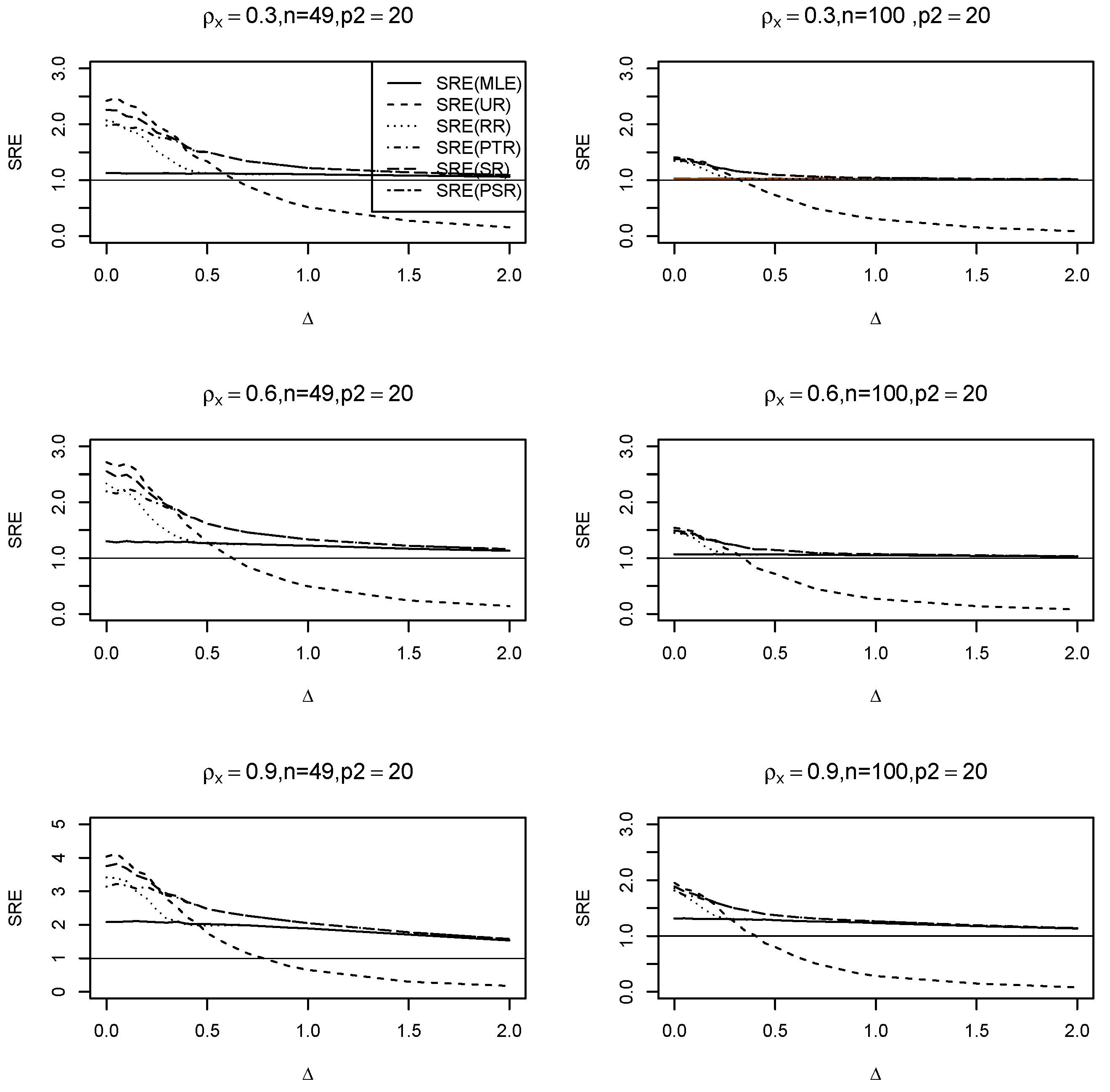
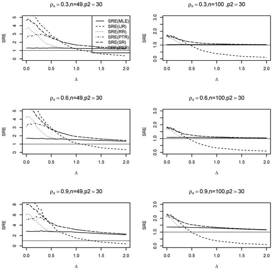
Figure A3.
SRE of the suggested estimators with respect to the MLE () for , , , and .
Figure A3.
SRE of the suggested estimators with respect to the MLE () for , , , and .
References
- Dai, X.; Li, E.; Tian, M. Quantile regression for varying coefficient spatial error models. Commun. Stat.—Theory Methods 2019, 50, 2382–2397. [Google Scholar] [CrossRef]
- Higazi, S.F.; Abdel-Hady, D.H.; Al-Oulfi, S.A. Application of spatial regression models to income poverty ratios in Middle Delta contiguous counties in Egypt. Pak. J. Stat. Oper. Res. 2013, 9, 93. [Google Scholar] [CrossRef]
- Piscitelli, A. Spatial Regression of Juvenile Delinquency: Revisiting Shaw and McKay. Int. J. Crim. Justice Sci. 2019, 14, 132–147. [Google Scholar]
- Liu, R.; Yu, C.; Liu, C.; Jiang, J.; Xu, J. Impacts of haze on housing prices: An empirical analysis based on data from Chengdu (China). Int. J. Environ. Res. Public Health 2018, 15, 1161. [Google Scholar] [CrossRef] [PubMed]
- Yildirim, V.; Mert, K.Y. Robust estimation approach for spatial error model. J. Stat. Comput. Simul. 2020, 90, 1618–1638. [Google Scholar] [CrossRef]
- Cressie, N. Statistics for Spatial Data; John Wiley & Sons: Nashville, TN, USA, 1993. [Google Scholar]
- Cressie, N.; Wikle, C.K. Statistics for Spatio-Temporal Data; Wiley-Blackwell: Chichester, UK, 2011. [Google Scholar]
- Haining, R. Spatial Data Analysis: Theory and Practice; Cambridge University Press: Cambridge, UK, 2003. [Google Scholar]
- Al-Momani, M.; Riaz, M.; Saleh, M.F. Pretest and shrinkage estimation of the regression parameter vector of the marginal model with multinomial responses. Stat. Pap. 2022, 64, 2101–2117. [Google Scholar] [CrossRef]
- Lisawadi, S.; Ahmed, S.E.; Reangsephet, O. Post estimation and prediction strategies in negative binomial regression model. Int. J. Model. Simul. 2020, 41, 463–477. [Google Scholar] [CrossRef]
- Nkurunziza, S.; Al-Momani, M.; Lin, E.Y. Shrinkage and lasso strategies in high-dimensional heteroscedastic models. Commun. Stat.—Theory Methods 2016, 45, 4454–4470. [Google Scholar] [CrossRef]
- Hoerl, A.E.; Kennard, R.W. A new Liu-type estimator in linear regression model. Technometrics 1970, 12, 55–67. [Google Scholar] [CrossRef]
- Kejian, L. A new class of biased estimate in linear regression. Commun. Stat.—Theory Methods 1993, 22, 393–402. [Google Scholar] [CrossRef]
- Li, Y.; Yang, H. A new Liu-type estimator in linear regression model. Stat. Pap. 2010, 53, 427–437. [Google Scholar] [CrossRef]
- Arashi, M.; Kibria, B.M.G.; Norouzirad, M.; Nadarajah, S. Improved preliminary test and Stein-rule Liu estimators for the ill-conditioned elliptical linear regression model. J. Multivar. Anal. 2014, 126, 53–74. [Google Scholar] [CrossRef]
- Arashi, M.; Norouzirad, M.; Roozbeh, M.; Khan, N.M. A high-dimensional counterpart for the ridge estimator in multicollinear situations. Mathematics 2021, 9, 3057. [Google Scholar] [CrossRef]
- Al-Momani, M. Liu-type pretest and shrinkage estimation for the conditional autoregressive model. PLoS ONE 2023, 18, e0283339. [Google Scholar] [CrossRef] [PubMed]
- Mardia, K.V.; Marshall, R.J. Maximum likelihood estimation of models for residual covariance in spatial regression. Biometrika 1984, 71, 135–146. [Google Scholar] [CrossRef]
- Al-Momani, M.; Hussein, A.A.; Ahmed, S.E. Penalty and related estimation strategies in the spatial error model. Stat. Neerl. 2016, 71, 4–30. [Google Scholar] [CrossRef]
- Bivand, R. R packages for Analyzing Spatial Data: A comparative case study with Areal Data. Geogr. Anal. 2022, 54, 488–518. [Google Scholar] [CrossRef]
- Harrison, D.; Rubinfeld, D.L. Hedonic housing prices and the demand for Clean Air. J. Environ. Econ. Manag. 1978, 5, 81–102. [Google Scholar] [CrossRef]
- Gilley, O.W.; Pace, R.K. On the Harrison and Rubinfeld data. J. Environ. Econ. Manag. 1996, 31, 403–405. [Google Scholar] [CrossRef]
- Pace, R.K.; Gilley, O.W. Using the Spatial Configuration of the Data to Improve Estimation. J. Real Estate Financ. Econ. 1997, 14, 333–340. [Google Scholar] [CrossRef]
- Solow, A.R. Bootstrapping correlated data. J. Int. Assoc. Math. Geol. 1985, 17, 769–775. [Google Scholar] [CrossRef]
- Boonstra, P.S.; Mukherjee, B.; Taylor, J.M. A small-sample choice of the tuning parameter in ridge regression. Stat. Sin. 2015, 23, 1185. [Google Scholar] [CrossRef] [PubMed]
- Seber, G.A.F. Spatial Data Analysis: Theory and Practice. In A Matrix Handbook for Statisticians; John Wiley & Sons: Hoboken, NJ, USA, 2008. [Google Scholar]
- Lee, L. Best Spatial Two-Stage Least Squares Estimators for a Spatial Autoregressive Model with Autoregressive Disturbances. Econom. Rev. 2003, 22, 307–335. [Google Scholar] [CrossRef]
- Liu, S.F.; Yang, Z. Asymptotic Distribution and Finite Sample Bias Correction of QML Estimators for Spatial Error Dependence Model. Econometrics 2015, 3, 376–411. [Google Scholar] [CrossRef]
- Yuzbasi, B.; Arashi, M.; Ahmed, S.E. Shrinkage estimation strategies in generalized ridge regression models under low/high-dimension regime. Int. Stat. Rev. 2020, 88, 229–251. [Google Scholar] [CrossRef]
- Fu, W.; Knight, K. Asymptotics for lasso-type estimators. Ann. Stat. 2000, 28, 1356–1378. [Google Scholar] [CrossRef]
- Judge, G.G.; Bock, M.E. The Statistical Implications of Pre-Test and Stein-Rule Estimators in Econometrics; North-Holland Pub. Co.: Amsterdam, The Netherlands, 1978. [Google Scholar]
Disclaimer/Publisher’s Note: The statements, opinions and data contained in all publications are solely those of the individual author(s) and contributor(s) and not of MDPI and/or the editor(s). MDPI and/or the editor(s) disclaim responsibility for any injury to people or property resulting from any ideas, methods, instructions or products referred to in the content. |
© 2024 by the authors. Licensee MDPI, Basel, Switzerland. This article is an open access article distributed under the terms and conditions of the Creative Commons Attribution (CC BY) license (https://creativecommons.org/licenses/by/4.0/).