Abstract
In global optimization problems, diversification approaches are often necessary to overcome the convergence toward local optima. One approach is the multi-start method, where a set of different starting configurations are taken into account to designate the best local minimum returned by the multiple optimization procedures as the (possible) global optimum. Therefore, parallelization is crucial for multi-start. In this work, we present a new multi-start approach for gradient-based optimization methods that exploits the reverse Automatic Differentiation to perform efficiently. In particular, for each step, this Automatic Differentiation-based method is able to compute the N gradients of N optimization procedures extremely quickly, exploiting the implicit parallelization guaranteed by the computational graph representation of the multi-start problem. The practical advantages of the proposed method are illustrated by analyzing the time complexity from a theoretical point of view and showing numerical examples where the speed-up is between and , with respect to classic parallelization methods. Moreover, we show that our AD-based multi-start approach can be implemented by using tailored shallow Neural Networks, taking advantage of the built-in optimization procedures of the Deep Learning frameworks.
MSC:
90C26; 90C30; 90C35; 65Y20
1. Introduction
Multi-start methods [1,2,3,4,5] are approaches used to increase the possibility of finding a global optimum instead of a local optimum in global optimization problems. This family of methods consists of making comparisons between many local optima obtained by running a chosen optimization procedure with respect to different starting configurations. Alternatively, multi-start is adopted when a set of local optima is desired by the optimization task. For these reasons, multi-start methods can be applied both to unconstrained and constrained optimization, both to derivative-free and derivative-based procedures, and both to meta-heuristic and theoretical-based optimization methods.
In global optimization problems, other approaches include population-based methods, like Genetic Algorithms (see, [6,7,8,9]) and Swarm Intelligence-based methods (e.g., Particle Swarm Optimization methods, see [10,11,12]). These nature-inspired methods are somehow similar to multi-start methods since they are based on a set of starting guesses; however, this set is used as a swarm of interacting agents that move in the domain of the loss function, looking for a global minimizer. Even if these latter methods are very efficient, they suffer a lack of understanding of the convergence properties, and it is not clear how much their efficiency is preserved if applied to large-scale problems [13]. Therefore, in high-dimensional domains, multi-start methods based on optimization procedures with well-known convergence properties can be preferred.
In the literature, sometimes the term multi-start is used to denote general global search methods, e.g., a random search or a re-start method can be defined as multi-start (see [14]), or vice-versa (see [15]). Nonetheless, in this work and according to [5], we denote as multi-start methods only those methods that consist in running the same optimization procedure with respect to a set of distinct starting points . Obviously, this approach can be modified into more specialized and sophisticated methods (e.g., [15,16,17,18]), but it is also useful in its basic form; indeed, it is implemented even in the most valuable computational frameworks (e.g., see [19]). However, the main difficulty of using a multi-start approach is that the number N of starting points typically must be quite large, due to the unknown number of local minima. For this reason, parallel computing is very important in this context, and the real exploitation of multi-start seems to be restricted to specific algorithms that are able to take advantage of the computer hardware for parallelization [16,17,20,21]. According to [21,22], three main parallelization approaches can be determined: (i) parallelization of the loss function computation and/or the derivative evaluations; () parallelization of the numerical methods performing the linear algebra operations; and () modifications of the optimization algorithms in a manner that improves the intrinsic parallelism (e.g., the number of parallelizable operations). In this work, we focus on the parallelization schemes of the first case (i), specifically on the parallelization of the derivative evaluations, because they are typically used for generating general purpose parallel software [21].
The main drawback of parallelization for multi-start methods is the difficulty of finding a trade-off between efficiency and easy implementation, especially for solving optimization problems of moderate dimensions on non-High Performance Computing (non-HPC) hardware. Typically, the simplest parallelization approach consists in distributing the computations among the available machine workers (e.g., via routines as [23,24]); however, very rarely is this also the most efficient method. Alternatively, a parallel program specifically designed for the optimization problem and for the hardware can be developed, but the time spent in writing this code may not be worth it. Of course, the cost of the parallelization of the derivative evaluations also depends on the computation methods used; when the gradient of the loss function is not available, Finite Differences are typically adopted in literature but, as observed in [22], the advent of Automatic Differentiation in recent decades has presented new interesting possibilities, allowing for the adoption of this technique for gradient computation in optimization procedures (e.g., see [25,26,27,28,29]).
The reverse Automatic Differentiation (AD), see [30] (Ch. 3.2)), was originally developed by Linnainmaa [31] in the 1970s, to be re-discovered by Neural Network researchers (who were not aware of the existence of AD [32]) in the 1980s under the name of backpropagation [33]. Nowadays, reverse AD characterizes almost all the training algorithms for Deep Learning models [32]. AD is a numerical method useful for computing the derivatives of a function, through its representation as an augmented computer program made of a composition of elementary operations (arithmetic operations, basic analytic fuctions, etc.) for which the derivatives are known. Then, using the chain rule of calculus, the method combines these derivatives to compute the overall derivative [32,34]. In particular, AD is divided into two sub-types: forward and reverse AD. The forward AD, developed in the 1960s [35,36], conceptually is the simplest one; it computes the partial derivative of a function by recursively applying the chain rule of calculus with respect to the elementary operations of f. On the other hand, reverse AD [31,33] “backwardly” reads the composition of elementary operations constituting the function f; then, still exploiting the chain rule of calculus, it computes the gradient . Both the AD methods can be extended to vectorial functions and used for computing the Jacobian. Due to the nature of the two AD methods, usually the reverse AD is more efficient if because it can compute the gradient of the j-th output of at once; otherwise, if , the forward AD is the more efficient method because it computes the partial derivatives with respect to for all the outputs of at once (see [30] (Ch. 3)). The characteristic described above for the reverse AD is the base for the new multi-start method proposed in this work, where we focus on the unconstrained optimization problem of a scalar function .
To improve the efficiency in exploiting the chain rule, the computational frameworks focused on AD (e.g., [37]) are based on computational graphs, i.e., they compile the program as a graph where operations are nodes and data “flow” through the network [38,39,40]. This particular configuration guarantees high parallelization and high efficiency (both for function evaluations and for AD-based derivative computations). Moreover, the computational graph construction is typically automatic and optimized for the hardware available, keeping the implementation relatively simple.
In this paper, we describe a new efficient multi-start method where the parallelization is not explicitly defined, thanks to the reverse Automatic Differentiation (see [30] (Ch. 3.2)) and the compilation of a computational graph representing the problem [39,40]. The main idea behind the proposed method is to define a function such that , for any set of vectors in , where is the loss function of the optimization problem and N is fixed. Since the gradient of G with respect to is equivalent to the concatenation of the N gradients , by applying the reverse AD on G we can compute the N gradients of the loss function very efficiently; therefore, we can implicitly and efficiently parallelize a multi-start method of N procedures running one AD-based optimization procedure for the function G. The main advantage of this approach is the good trade-off between efficiency and easy implementation. Indeed, nowadays the AD frameworks (e.g., [37]) compile functions and programs as computational graphs that automatically but very efficiently exploit the available hardware; then, with the proposed method, the user just needs to define the function G and the differentiation through the reverse AD, obtaining a multi-start optimization procedure that (in general) is more time-efficient than a direct parallelization of the processes, especially excluding an HPC context. Moreover, the method can be extended, implementing it by using tailored shallow Neural Networks and taking advantage of the built-in optimization procedures of the Deep Learning frameworks.
The work is organized as follows. In Section 2, we briefly recall and describe the AD method. In Section 3, we start introducing a new formulation of the multi-start problem that is useful for the exploitation of the reverse AD, and the time complexity estimations are illustrated. Then, we show numerical results illustrating a context where the proposed method is advantageous with respect to a classic parallelization. In Section 4, we show how to implement the AD-based multi-start approach using a tailored shallow Neural Network (NN) in those cases where the user wants to take advantage of the optimization procedures available in most of the Deep Learning frameworks. In particular, we illustrate an example where the new multi-start method is implemented as a shallow NN and used to find three level set curves of a given function. Finally, some conclusions are drawn in Section 5.
2. Automatic Differentiation
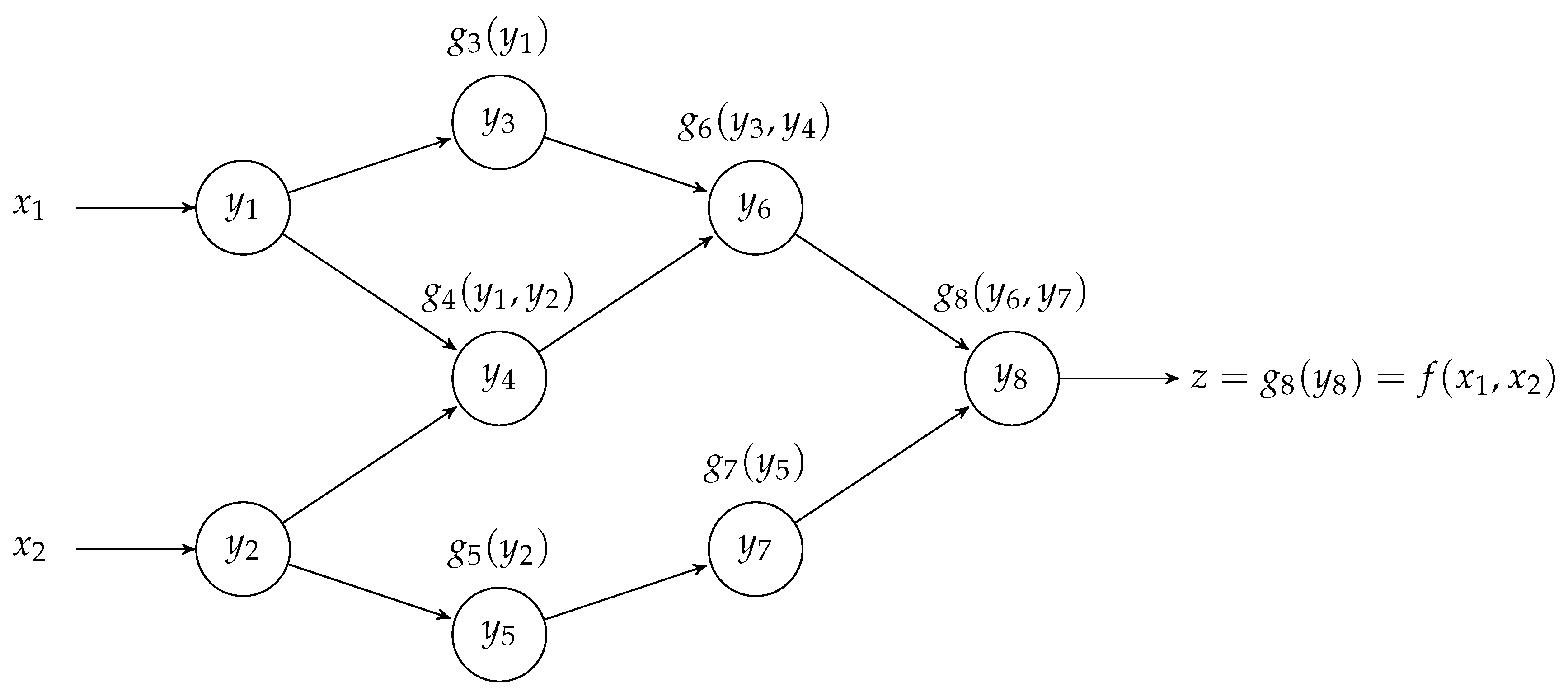
Automatic Differentiation (AD) is a numerical method to compute the exact derivatives of a function, representing it as an augmented computer program made of a composition of elementary operations for which the derivatives are known [30] (Ch. 3.2); typically, this program is represented as a graph connecting the elementary operations (e.g., see Figure 1).

Figure 1.
Example of computational graph representing as a composition of elementary functions .
The first idea about AD dates back to the 1950s [35], and the forward mode AD was developed in the 1960s [36]. In the 1970s, Linnainmaa developed the reverse mode AD [31]. This latter method is equivalent to the one independently developed by NN researchers in the late 1980s, with the name of backpropagation [33]. Nowadays, backpropagation is recognized as the application of the reverse mode AD for derivatives computation in NNs.
2.1. Forward Mode AD
The forward AD is conceptually the simplest of the two methods. Given a scalar function , this method consists of a recursive application of the chain rule of calculus for computing the partial derivative , for a fixed . More specifically, let us us assume that f is the result of a composition of M elementary operations with known derivatives. Let us denote with the intermediate variables such that , for each , and is the result of the elementary operation applied to a subset of “previous” intermediate variables, for each ; for the ease of notation, we use the same index j both for the elementary operation and the intermediate variable returned by it (see Figure 1).
Now, let be a fixed input variable and . Then, it holds that
where the term “parent of” refers to the computational graph of f (see Figure 1). Then, we can build another “composition graph” with the same connectivity of the one of f but with elementary operations given by (1). Therefore, given a vector , we can compute the value of the derivative with the following steps:
- We compute , and we store all the intermediate variable values involved in the computations of the second “forward AD graph”;
- We compute the output value of the forward AD graph, giving as input (a.k.a. seed) the canonical basis vector (i.e., selecting as input variable for the partial derivatives).
2.2. Reverse Mode AD
The reverse mode of AD “backwardly” reads the connections of the composition graph of the function to exploit the differentiation dependencies. This procedure is somehow equivalent to “exploding” the partial derivatives and identifying their elementary functions. Let us introduce the following quantities:
Then, for each , the following holds:
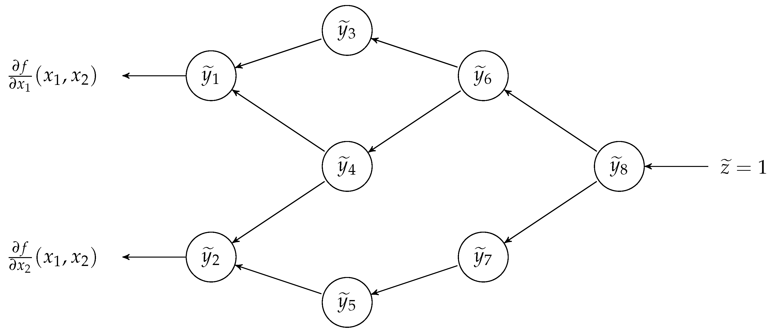
It is easy to observe that the differentiation dependencies written in (2) are evident when reading the computational graph of f (see Figure 1) from right to left. Then, the reverse mode AD consists of building another composition graph that has the same connectivity but is executed in the opposite way and where the elementary operations are given by (2). If we consider the example function of Figure 1, we can build the “reverse AD graph” illustrated in Figure 2.

Figure 2.
Example of reverse AD computational graph for f as in Figure 1.
Then, given a vector , we can compute the value of the entire gradient with the following steps:
- We compute , and we store all the intermediate variable values involved in the computations of the reverse AD graph;
- We compute the output values of the function represented by the reverse AD graph, giving as the seed the scalar value equal to 1 (i.e., ).
2.3. Automatic Differentiation for Jacobians
AD can be easily extended to vectorial functions [30] (Ch. 3.2). In particular, given a vector , the Jacobian matrix at can be computed running m times the reverse AD, using the m canonical basis vectors as seeds to the reverse AD graph; alternatively, it can be computed n times running the forward AD, using the n canonical basis vectors as seeds to the forward AD graph. In other words, the reverse AD graph with input vector returns the j-th row of the Jacobian matrix, while the forward AD graph with input vector returns the i-th column of the Jacobian matrix. For these reasons, in general the reverse AD is more efficient if ; otherwise, if , the forward AD is the more efficient method.
Focusing on scalar functions, it is trivial to observe that we can compute the gradient running once the reverse AD instead of running the forward one n times.
3. Reverse Automatic Differentiation for Multi-Start
Let us consider the unconstrained optimization problem
where is a given function, and let us approach the problem with a gradient-based optimization method (e.g., the steepest descent). Moreover, we assume f is the composition of elementary operations so that it is possible to use the reverse AD to compute its gradient.
The main idea behind the reverse AD-based multi-start method is to define a function such that it is a linear combination of loss function evaluations at N vectors, i.e.,
for each , fixed, . Then, for any set of points where f is differentiable, the gradient of G at is equal to the concatenation of the vectors . Therefore, using the reverse AD to compute the gradient , we obtain a very fast method to evaluate the N exact gradients , where denotes the domain variable of G in . Therefore, we can apply the steepest descent method for G, which actually corresponds to applying N times the steepest descent methods to f. In the following, we formalize this idea.
Definition 1 (-concatenation).
For each fixed , for any function , a function is an N-concatenation of if
for each set of N vectors .
Notation 1.
For the sake of simplicity, from now on vectors will be denoted by . Analogously, vectors returned by an N-concatenation of a function will be denoted by .
Definition 2 (-concatenation).
For each fixed , for any function , a function is a λ-concatenation of if
for each set of N vectors .
Remark 1.
Obviously, an N-concatenation of is a λ-concatenation of with .
Given these definitions, the idea for the new multi-start method is based on the observation that the steepest descent method for G, starting from and with step-length factor , represented by
is equivalent to
if the gradient of G is an N-concatenation of the gradients of f, i.e,
Analogously, if the gradient of G is a -concatenation of the gradients of f, with , , then (6) is equivalent to
i.e., is equivalent to applying N times the steepest descent methods to f, with step-length factors .
Remark 2 (Extension to other gradient-based methods).
It is easy to see that we can generalize these observations to other gradient-based optimization methods than the steepest descent (e.g., momentum methods [41,42]). Let be the function characterizing the iterations of a given gradient-based method, i.e, such that
for each , each step-length and each objective function . Then, the iterative process for G, starting from , and with respect to a gradient-based method characterized by is
that is equivalent to the multi-start approach with respect to f:
Moreover, we can further extend the generalization if we assume that, for each and each , the following holds:
where is a fixed function. Indeed, if the gradient of G is a λ-concatenation of the gradients of f, Equation (12) changes into
where , for each .
3.1. Using the Reverse Automatic Differentiation
To actually exploit the reverse AD for a multi-start steepest descent (or another gradient-based method), we need to define a function G with gradient a -concatenation of the gradients of f, the objective function of problem (3).
Proposition 1.
Let us consider a function . Let be an N-concatenation of f, for a fixed , and let be the linear function
for a fixed , .
Then, for each set of points where f is differentiable, the gradient of the function is a λ-concatenation of the gradient of f.
Proof.
The proof is straightforward since
for each set of points where f is differentiable. □
Assuming that the expression of is unknown, a formulation such as (14) obtained from seems to give no advantages without AD and/or tailored parallelization. Indeed, the computation of the gradient through classical gradient approximation methods (e.g., Finite Differences) needs N different gradient evaluations for each point , respectively, and each one of them needs function evaluations (assuming no special structures for f); then, e.g., the time complexity of the gradient approximation with Finite Differences for G (denoted by ) is
where denotes the time complexity.
On the other hand, reverse AD permits the efficient operation of the gradient-based method (11), equivalent to the N gradient-based methods, even for large values of n and N. Indeed, from [30] (Ch. 3.3), for any function , it holds that the time complexity of a gradient evaluation of g with reverse AD (in a point where the operation is defined) is such that
where denotes the gradient computed with reverse AD. The following lemma characterizes the relationship between the time complexity of and the time complexity of f.
Lemma 1.
Let f, , and be as in Proposition 1. Let be such that , and let us assume that
Then, the time complexity of is
Comparing (19) and the time complexity (16) of the Finite Differences gradient approximation, we observe that reverse AD is much more convenient both because it computes the exact gradient and because of the time complexity. In the following example, we illustrate the concrete efficiency of using to compute N gradients of the n-dimensional Rosenbrock function, assuming its gradient is unknown.
Example 1 (Reverse AD and the -dimensional Rosenbrock function).
Let be the n-dimensional Rosenbrock function [43,44,45]:
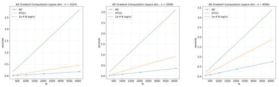
Assuming a good implementation of f, we have that the time complexity of the function is . Then, it holds that . In this particular case, we observe that the coefficient , such that
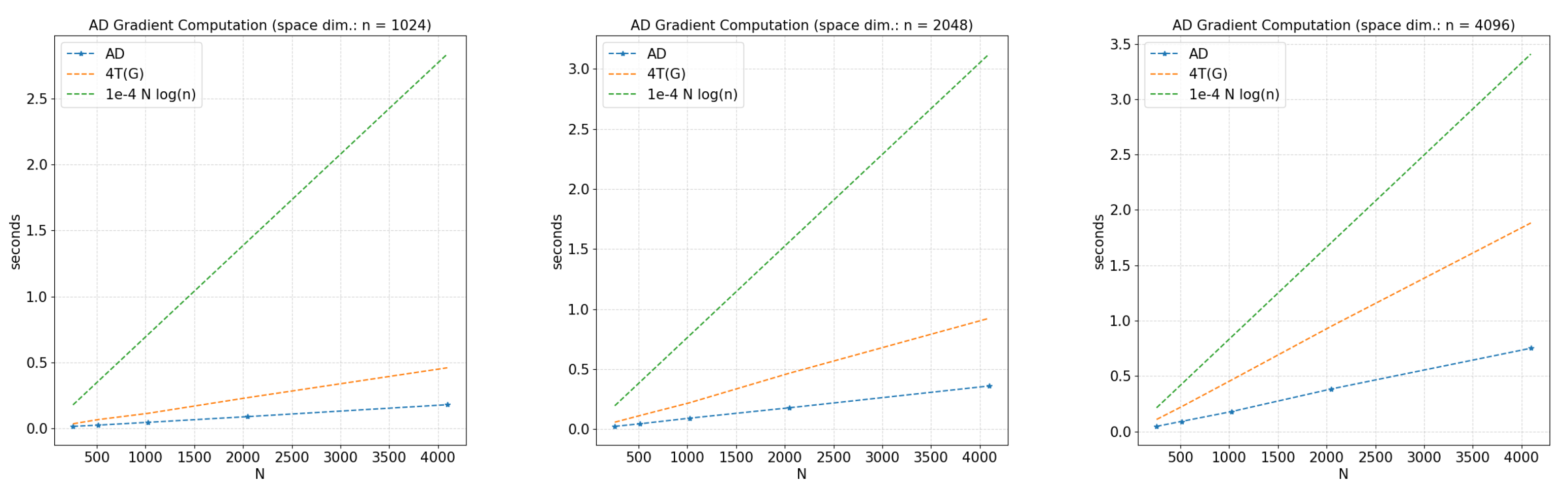
for sufficiently large N and n is very small; specifically, for the given example, we have ; moreover, we observe that the reverse AD can compute gradients of f in a space of dimension in less than one second (see Figure 3). All the computations are performed using a Notebook PC with Intel Core i5 Processor dual-core (2.3 GHz) and 16 GB DDR3 RAM.
Figure 3.
Average computation time of the reverse AD method (blue curves) with respect to four times the average computation time of G (orange curves) and the curve , for each fixed (from left to right).
3.2. An Insight into AD and Computational Graphs
Equation (19) of Lemma 1 tells us that the time complexity of computing N times the gradient is ; then, with a proper parallelization procedure of these N gradient computations, the construction of G seems to be meaningless. However, the special implementation of G as a computational graph, made by the frameworks used for AD (see Section 1), guarantees an extremely efficient parallelization, both for the evaluation of G and the computation of . For example, during the graph compilation, the framework TensorFlow [37] identifies separate sub-parts of the computation that are independent and splits them [40], optimizing the code execution “aggressively” [39]; in particular, this parallelization does not consist only in sending sub-parts to different machine workers but also in optimizing the data reading procedure such that each worker can perform more operations almost at the same time (similarly to implementations that exploit vectorization [46]). Then, excluding a High-Performance Computing (HPC) context, the computational graphs representing G and make the AD-based multi-start method (almost always) more time-efficient than a multi-start method where the code explicitly parallelizes the N gradient computations of or the N optimization procedures (see Section 3.3 below); indeed, in the parallelized multi-start case, each worker can compute only one gradient/procedure at a time, and the number of workers is typically less than N. Moreover, the particular structure of the available frameworks makes the implementation of the AD-based method very easy.
As written above, the time-efficiency properties of a computational graph are somehow similar to the ones given by the vectorization of an operation; we recall that the vectorization (e.g., see [46]) of a function is the code implementation of f as a function such that, without the use of for/while-cycles, the following holds:
for each matrix , , and where denotes the transposed i-th row of X. In this case, especially when , using is much more time-efficient than parallelizing N computations of f, thanks to the particular data structure read by the machine workers, which is optimized according to memory allocation, data access, and workload reduction. Therefore, we easily deduce that the maximum efficiency for the AD-based method is obtained when G is built using instead of (if possible).
Summarizing the content of this subsection, the proposed AD-based multi-start method exploits formulation (6) to build an easy and handy solution for an implicit and highly efficient parallelization of the procedure, assuming access to AD frameworks.
3.3. Numerical Experiments
In this section, we illustrate the results of a series of numerical experiments that compare the computational costs (in time) of three multi-start methods for problem (3):
- (i)
- AD-based multi-start steepest descent, exploiting vectorization (see Section 3.2);
- ()
- AD-based multi-start steepest descent, without exploiting vectorization;
- ()
- Parallel multi-start steepest descent, distributing the N optimization procedures among all the available workers. In this case, the gradient of f is computed using the reverse AD, for a fair comparison with case (i) and case ().
The experiments have been performed using a Notebook PC with Intel Core i5 Processor dual-core (2.3 GHz) and 16 GB DDR3 RAM (see Example 1); in particular, each multi-start method has been executed alone, as the unique running application on the PC (excluded mandatory applications in the background). The methods are implemented in Python, using the TensorFlow module for reverse AD; the parallelization of method () is based on the multiprocessing built-in module [24].
Since we want to analyze the time complexity behavior of the three methods varying the domain dimension n and the number of starting points N, we perform the experiments considering the Rosenbrock function (see (20), Example 1). This function is particularly suitable for our analyses since its expression is defined for any dimension , and it has always a local minimum in .
According to the different natures of the three methods considered, the implementation of the Rosenbrock function changes. In particular, for method (i), in the AD framework we implement a function G that highly exploit vectorization, avoiding any for-cycle (see Algorithm 1); for method (), we implement G cycling among the set of N vectors with respect to which we must compute the function (see Algorithm 2); for method (), we do not implement G, only the Rosenbrock function (see Algorithm 3).
| Algorithm 1 G-Rosenbrock implementation—Method (i) |
| Input: X, matrix of columns, of rows; Output: y, output scalar value of G built with respect to (20).
|
We test the three methods varying all the combinations of N and n, with and , for a total number of 50 experiments. The parameters of the steepest descent methods are fixed: , maximum number of iterations , stopping criterium’s tolerance for the gradient’s norm, and fixed starting points sampled from the uniform distribution ; computations are performed in single precision, the default precision of TensorFlow. The choice of a small value for , together with the sampled starting points, and the “flat” behavior of the function near to the minimum ensure that the steepest descent methods always converge toward using all the iterations allowed, i.e., but , for each .
| Algorithm 2 G-Rosenbrock implementation—Method () |
| Input: X, matrix of columns, of rows; Output: y, output scalar value of G built with respect to (20).
|
| Algorithm 3 Rosenbrock implementation—Method () |
| Input: x, vector in ; Output: y, output scalar value of (20).
|
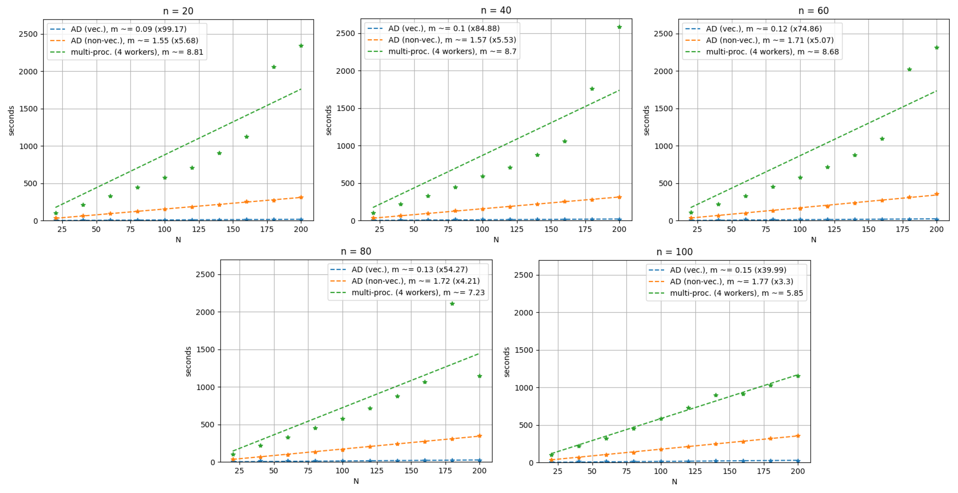
Looking at the computation times of the methods, reported in Table 1, Table 2 and Table 3 and illustrated in Figure 4, the advantage of using the AD-based methods is evident, in particular when combined with vectorization; indeed, we observe that in its slowest case, , method (i) is still faster than the fastest case, , of both method and method .

Table 1.
Method (i). AD-based multi-start plus vectorization. Computation times w.r.t. N starting points in , iterations. Time notation: minutes:seconds.decimals.
Table 2.
Method (). AD-based multi-start, no vectorization. Computation times w.r.t. N starting points in , iterations. Time notation: minutes:seconds.decimals.
Table 3.
Method (). Parallel multi-start (four workers). Computation times w.r.t. N starting points in , iterations. Time notation: minutes:seconds.decimals.
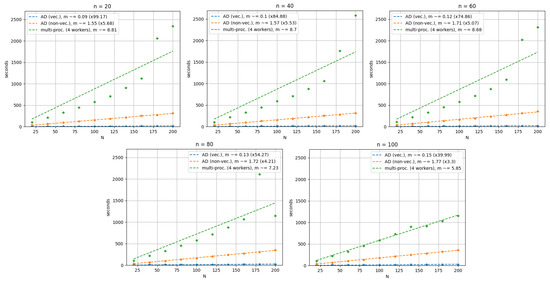
Figure 4.
Cases , from left to right, from top to bottom. Computation times w.r.t. N starting points in of method (i) (blue color), method () (orange color), and method () (green color). Dots are the computation times (in seconds) of the methods w.r.t. . Lines describe the linear time complexity behaviour of the methods. The value m in the legends denotes the angular coefficient of the approximating lines.
The linear behaviour of the methods’ time complexity with respect to N is confirmed (see Figure 4); however, the parallel multi-start method’s behavior is afflicted by higher noise, probably caused by the machine’s management of the jobs’ queue. Nonetheless, the linear behaviors of the methods are clearly different: the AD-based multi-start methods are shown to be faster than the parallel multi-start method, with a speed-up factor between and (method ()) and between and (method (i)).
3.4. Scalability and Real-World Applications
The experiments illustrated in the subsection above are a good representation of the general behavior that we can expect to observe in a real-world scenario, even further increasing the number n of dimensions and/or the number N of optimization procedures.
We recall that the we are assuming that the loss function f is the composition of known elementary operations, so that it is possible to use AD frameworks for the implementation of G (built on f). Under these assumptions, the experiments with the Rosenbrock function are a good representation of the general behavior of the proposed method with respect to a “classically parallelized” multi-start approach. Indeed, the main difference is only in the elementary operations necessary for implementing f and G, varying the time complexity . Therefore, even in the worst case of no vectorization of f and/or G, the experiments show that the AD-based method is faster with respect to the parallelized multi-start (see method () and method ()). Moreover, the implementation of the AD-based method is much simpler; indeed, the user needs only to run one optimization procedure on the function G instead of writing a code for optimally parallelizing N procedures with respect to f.
Our AD-based approach is intended to be an easy, efficient, and implicit parallelization of a general purpose multi-start optimization procedure, applicable to problems with f that are relatively simple to define/implement and typically solved by excluding an HPC context. On the other hand, for highly complex and expensive optimization problems and/or loss functions, a tailored parallelization of the multi-start procedure is probably the most efficient approach, possibly designed for that specific optimization problem and run on an HPC. Of course, the AD-based method cannot be applied to optimization problems with a loss function that is not implementable in an AD framework.
3.5. Extensions of the Method and Integration in Optimization Frameworks
The proposed AD-based multi-start method has been developed for general gradient-based optimization methods for unconstrained optimization (see Remark 2). Nonetheless, it has the potential to be extended to second-order methods (e.g., via matrix-free implementations [47] (Ch. 8)) and/or to constrained optimization. Theoretically, the method is also relatively easy to be integrated in many existing optimization frameworks or software tools, especially if they already include AD for evaluating derivatives (e.g., see [29]); indeed, the user just needs to apply these tools/frameworks with respect to the function G, instead of f, by asking to compute the gradient with reverse AD. Moreover, as we will see in the next section, the AD-based method can also take advantage of the efficient training routines of the Deep Learning frameworks for solving optimization problems.
However, the extensions mentioned above need further analysis before being implemented, and some concrete limitations for the method still exist. For example, line-search methods (e.g., see [47,48,49,50]) for the step-lengths of the N multi-start procedures have not been considered yet; indeed, the current formulation has only one shared step-length for all the N procedures. Similarly, distinct stopping criteria for the procedures are not defined. In future work, we will extend the AD-based multi-start method to the cases listed in this subsection.
4. Multi-Start with Shallow Neural Networks
In this section, we show how to exploit the available Neural Network (NN) frameworks to build a shallow NN that, trained on fake input–output pairs, performs a gradient-based optimization method with respect to N starting points and a given loss function function f. Indeed, the usage of NN frameworks (typically, coincident with or part of AD frameworks) let us exploit the already implemented gradient-based optimization methods defined for NN training, also taking advantage of their highly optimized code implementation. Therefore, from a practical point of view, this approach is useful to easily implement a reverse AD-based multi-start method with respect to the built-in optimizers of the many available NN frameworks.
In the following definition, we introduce the archetype of such a NN. Then, we characterize its use with two propositions, to explain how to use the NN for reverse AD-based multi-start.
Definition 3 (Multi-Start Optimization Neural Network).
Let be a loss function, and let be an NN with the following architecture:
- 1.
- One input layer of n units;
- 2.
- One layer of N units and fully connected with the input layer. In particular, for each , the unit of the layer returns a scalar outputwhere is the vector of the weights of the connections between the input layer units and .
Then, we define as multi-start optimization NN (MSO-NN) of N units with respect to f.
Remark 3.
We point the reader to the fact that (21) does not depend on the NN inputs but only on the layer weights. Then, an MSO-NN does not change its output, varying the inputs. The reasons behind this apparently inefficient property are explained in the next propositions.
Proposition 2.
Let be an MSO-NN of N units with respect to f. Let us endow with a training loss function ℓ such that,
for any input–output pair , where is fixed, and denotes the vector collecting all the weights of . Moreover, for the training process, let us endow with a gradient-based method that exploits the backpropagation, defined as in Remark 2.
Given N vectors , let us initialize the weights of such that the weight vector is equal to , for each and . Then,
Proof.
Since the second item is a direct consequence of the first item, we prove only item 1.
The optimization method for the training of is characterized by a function that satisfies (10) and (13). Then, the training of consists of the following iterative process that updates the weights:
independently of the data used for the training (see (22)). We recall that denotes the gradients computed with reverse AD and that it is used in (23) because the optimization method exploits the backpropagation for hypothesis.
Now, by construction, we observe that , with and defined as in Proposition 1. Then, due to Proposition 1 and Remark 2, the thesis holds.
□
Proposition 3.
Let be as in the hypotheses of Proposition 2, with the exception of the loss function ℓ that is now defined as
for any input–output pair and where is fixed. Let be a training set where the input–output pairs have fixed output . Then,
- 1.
- Given the training set , the updating of the weights of at each training epoch is equivalent to the multi-start step (14) applied to the merit function , computed with reverse AD and such that ;
- 2.
- For each , the weights of , after training epochs, are such thatwhere are the vectors defined by the multi-start process of item 1.
Proof.
The proof is straightforward, from the proof of Proposition 2. □
With the last proposition, we introduced the minimization of a merit function. The reason is that multi-start methods can be useful not only in looking for one global optimum but also when a set of global/local optima is asked for. An example is the level curve detection problem where, for a given function and a fixed , we look for the level curve set minimizing a merit function, e.g., . In this case, a multi-start approach is very important since the detection of more than one element of is typically sought (when is not empty or given by one vector only). In the next section, we consider this case problem for the numerical tests.
We conclude this section with remarks concerning the practical implementation of MSO-NNs.
Remark 4 (GitHub Repository and MSO-NNs).
The code for implementing an MSO-NN is available on GitHub (https://github.com/Fra0013To/AD_MultiStartOpt, accessed on 11 April 2024). The code of the example illustrated in Section 4.1 is reported and can be modified for adapting it to other optimization problems.
Remark 5 (Avoiding overflow).
In some cases, if the objective function f is characterized by large values, an overflow may occur while using an MSO-NN to minimize f with an AD-based multi-start approach. In particular, the overflow may occur during the computation of if the parameters are not small enough. One of the possible (and easiest) approaches is to select ; then, in the case illustrated in Proposition 3, it is equivalent to select ℓ as the Mean Square Error (MSE) loss function.
4.1. Numerical Example
In this section, we report the results about the use of an MSO-NN to find level curve sets of the Himmelblau function
The Himmelblau function [51] is characterized by non-negative values, with lower bound . In particular, f has four local minima:
these local minima are also global minima since , for each .
For our experiments, we consider an MSO-NN defined as in Proposition 3, with (see Remark 5). The NN is implemented using the TensorFlow (TF) framework [37], and we endow with the Adam optimization algorithm [52], the default algorithm for training NNs in TF, with a small and fixed step-length . We use Adam to show examples with a generic gradient-based method, and we set to emphasize the efficiency of the AD-based multi-start even when a large number of iterations are required to obtain the solutions.
Remark 6 (Adam satisfies (13)).
In these experiments, we can use the Adam optimization algorithm because Equation (13) holds for Adam, with . Actually, (13) holds from a theoretical point of view, due to a small parameter ϵ introduced in the algorithm to avoid zero division errors during the computations. Nonetheless, in practice, Proposition 3 and Remark 2 still hold for Adam if we set ϵ such that is sufficiently small (e.g., ).
Specifically, the Adam optimization algorithm updates the NN weights according to the rule
where all the operations are intended to be element-wise; and are the first and second bias-corrected moment estimates, respectively; and is a small constant value (typically ) to avoid divisions by zero [52]. Then, by construction (see [52]), we observe that the bias-corrected moment estimates with respect to a loss function ℓ are such that
where are the bias-corrected moment estimates with respect to another loss function such that , . Therefore, assuming and considering the effective step, the following holds:
on the other hand, assuming , the two methods are equivalent but characterized by different parameters to avoid divisions by zero, i.e.,
Finding Level Curve Sets of the Himmelblau Function
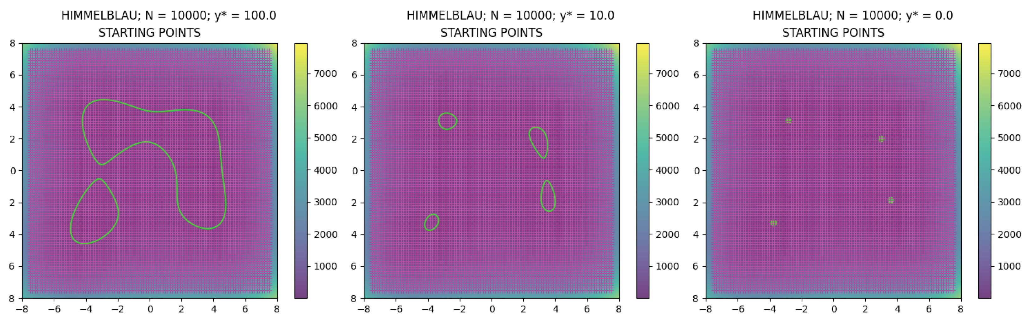
Given the MSO-NN described above, we show three cases of level-curve search: the case with (set denoted by ), the case with (set denoted by ), and the case with (set denoted by , see (26)); in particular, the latter case is equivalent to the global minimization problem of the function. For all the cases, for the multi-start method we select the points of the regular grid as starting points
where (see Figure 5). Then, for each , we train for epochs (i.e., K multi-start optimization steps), initializing the weights with . We recall that, for each , the -th training epoch of is equivalent to Adam optimization steps with respect to the vectors . The training is executed on a Notebook PC with Intel Core i5 Processor dual-core (2.3 GHz) and 16 GB DDR3 RAM (same PC of Example 1 and Section 3.3).
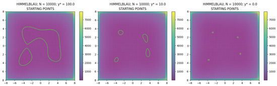
Figure 5.
Top view of the Himmelblau function in . The magenta crosses are the grid points of (31). In green, the level curve sets , , and (from left to right).
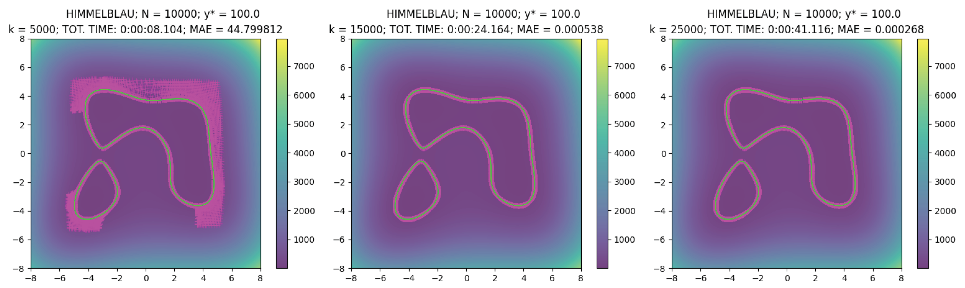
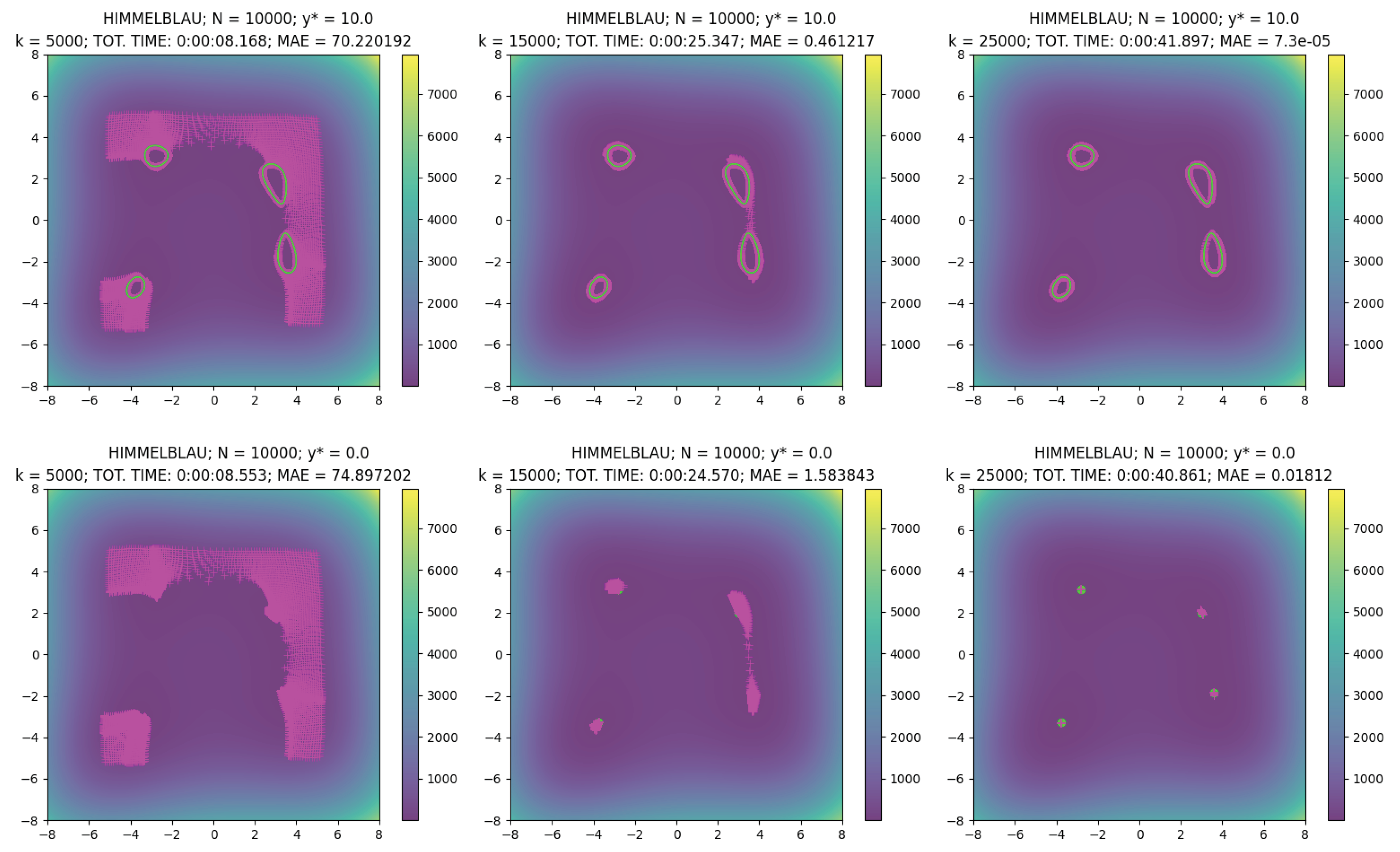
Now, for each k = 5000, 15,000, 25,000, in Table 4 we report the computation time and the Mean Absolute Error (MAE) of the points with respect to the target value , i.e.,
Table 4.
MAE of the points with respect to the target value and total computation time of k = 5000, 15,000, 25,000 iterations for the AD-based multi-start method using the MSO-NN .
Looking at the values in the table and at Figure 6, we observe the very good performances of the new multi-start method. Indeed, not only all the N sequences are convergent toward a solution, but we observe that the average time of one minimization step, characterized by the computation of gradients in , is equal to s. The result is interesting because the method is efficient without the need for defining any particular parallelization routine to manage the N optimization procedures at the same time.

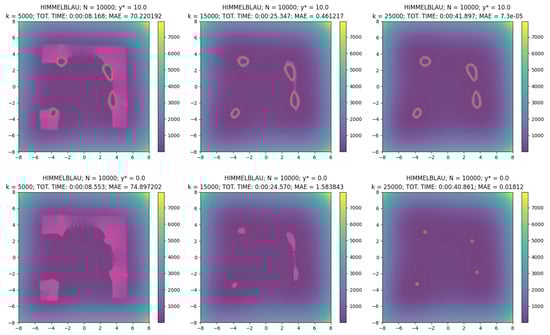
Figure 6.
Top view of the Himmelblau function in during the search of the level curve sets , , and (first, second, and third row, respectively), denoted by the green curves or dots. The magenta crosses are the points , with respect to iteration k = 5000, 15,000, 25,000 (from left to right).
5. Conclusions
We presented a new multi-start method for gradient-based optimization algorithms, based on the reverse AD. In particular, we showed how to write N optimization processes for a function as one optimization process for the function , computing the gradient with the reverse AD. Then, assuming no HPC availability, this problem formulation defines an easy and handy solution for an implicit and highly efficient parallelization of the multi-start optimization procedure.
Specifically, the method is not supposed to be applied to complex and expensive optimization problems, where detailed and tailored parallelized multi-start methods are probably the best choice; on the contrary, the AD-based multi-start method is intended to be an easy and efficient alternative for parallelizing general purpose gradient-based multi-start methods.
The efficiency of the method has been positively tested on a standard personal computer with respect to 50 cases of increasing dimension and the number of starting points obtained from an n-dimensional test function. These experiments have been performed using a naive steepest-descent optimization procedure.
We observed that the method has the potential to be extended to second-order methods and/or to constrained optimization. In the future, we will focus on extending the method to these cases and implementing custom line search methods and/or distinct stopping criteria for the N optimization procedures.
In the end, we presented a practical implementation of the AD-based multi-start method as a tailored shallow Neural Network, and we tested it on three different values for the level curve set identification problem on the Himmelblau function, where the latter one is equivalent to the global minimization problem. This example highlights another advantage of the new method: the possibility to use NNs for exploiting the already implemented and efficient gradient-based optimization methods defined in the NN frameworks for the models’ training.
Funding
This study was carried out within the FAIR-Future Artificial Intelligence Research and received funding from the European Union Next-GenerationEU (PIANO NAZIONALE DI RIPRESA E RESILIENZA (PNRR)–MISSIONE 4 COMPONENTE 2, INVESTIMENTO 1.3—D.D. 1555 11/10/2022, PE00000013). This manuscript reflects only the authors’ views and opinions; neither the European Union nor the European Commission can be considered responsible for them.
Institutional Review Board Statement
Not applicable.
Informed Consent Statement
Not applicable.
Data Availability Statement
Data are contained within the article.
Conflicts of Interest
The authors declare no conflicts of interest.
Sample Availability
Code samples are available at this link: https://github.com/Fra0013To/AD_MultiStartOpt, accessed on 21 March 2024.
Abbreviations
The following abbreviations and nomenclatures are used in this manuscript:
| AD | Automatic Differentiation |
| FD | Finite Differences |
| HPC | High-Performance Computing |
| MSO-NN | Multi-Start Optimization Neural Network |
| NN | Neural Network |
References
- Zieliński, R. A statistical estimate of the structure of multi-extremal problems. Math. Program. 1981, 21, 348–356. [Google Scholar] [CrossRef]
- Betrò, B.; Schoen, F. Sequential stopping rules for the multistart algorithm in global optimisation. Math. Program. 1987, 38, 271–286. [Google Scholar] [CrossRef]
- Piccioni, M.; Ramponi, A. Stopping rules for the multistart method when different local minima have different function values. Optimization 1990, 21, 697–707. [Google Scholar] [CrossRef]
- Betrò, B.; Schoen, F. Optimal and sub-optimal stopping rules for the Multistart algorithm in global optimization. Math. Program. 1992, 57, 445–458. [Google Scholar] [CrossRef]
- Schoen, F. Stochastic techniques for global optimization: A survey of recent advances. J. Glob. Optim. 1991, 1, 207–228. [Google Scholar] [CrossRef]
- Yang, X.S. Chapter 6-enetic Algorithms. In Nature-Inspired Optimization Algorithms, 2nd ed.; Yang, X.S., Ed.; Academic Press: Cambridge, MA, USA, 2021; pp. 91–100. [Google Scholar] [CrossRef]
- Mitchell, M. Elements of Generic Algorithms—An Introduction to Generic Algorithms; The MIT Press: Cambridge, MA, USA, 1998; p. 158. [Google Scholar] [CrossRef]
- Yadav, P.K.; Prajapati, N.L. An Overview of Genetic Algorithm and Modeling. Int. J. Sci. Res. Publ. 2012, 2, 1–4. [Google Scholar]
- Colombo, F.; Della Santa, F.; Pieraccini, S. Multi-Objective Optimisation of an Aerostatic Pad: Design of Position, Number and Diameter of the Supply Holes. J. Mech. 2019, 36, 347–360. [Google Scholar] [CrossRef]
- Kennedy, J.; Eberhart, R. Particle swarm optimization. In Proceedings of the ICNN’95-International Conference on Neural Networks, Perth, WA, Australia, 27 November–1 December 1995; Volume 4, pp. 1942–1948. [Google Scholar] [CrossRef]
- Yang, X.S. Chapter 8-Particle Swarm Optimization. In Nature-Inspired Optimization Algorithms, 2nd ed.; Yang, X.S., Ed.; Academic Press: Cambridge, MA, USA, 2021; pp. 111–121. [Google Scholar] [CrossRef]
- Isiet, M.; Gadala, M. Sensitivity analysis of control parameters in particle swarm optimization. J. Comput. Sci. 2020, 41, 101086. [Google Scholar] [CrossRef]
- Yang, X.S. Nature-inspired optimization algorithms: Challenges and open problems. J. Comput. Sci. 2020, 46, 101104. [Google Scholar] [CrossRef]
- Martí, R. Multi-Start Methods. In Handbook of Metaheuristics; Glover, F., Kochenberger, G.A., Eds.; Springer: Boston, MA, USA, 2003; pp. 355–368. [Google Scholar] [CrossRef]
- Hu, X.; Spruill, M.C.; Shonkwiler, R.; Shonkwiler, R. Random Restarts in Global Optimization; Technical Report; Georgia Institute of Technology: Atlanta, Georgia, 1994. [Google Scholar]
- Bolton, H.; Groenwold, A.; Snyman, J. The application of a unified Bayesian stopping criterion in competing parallel algorithms for global optimization. Comput. Math. Appl. 2004, 48, 549–560. [Google Scholar] [CrossRef]
- Peri, D.; Tinti, F. A multistart gradient-based algorithm with surrogate model for global optimization. Commun. Appl. Ind. Math. 2012, 3, e393. [Google Scholar] [CrossRef]
- Mathesen, L.; Pedrielli, G.; Ng, S.H.; Zabinsky, Z.B. Stochastic optimization with adaptive restart: A framework for integrated local and global learning. J. Glob. Optim. 2021, 79, 87–110. [Google Scholar] [CrossRef]
- Mathworks. MultiStart (Copyright 2009–2016 The MathWorks, Inc.). Available online: https://it.mathworks.com/help/gads/multistart.html (accessed on 11 April 2024).
- Dixon, L.C.; Jha, M. Parallel algorithms for global optimization. J. Optim. Theory Appl. 1993, 79, 385–395. [Google Scholar] [CrossRef]
- Migdalas, A.; Toraldo, G.; Kumar, V. Nonlinear optimization and parallel computing. Parallel Comput. 2003, 29, 375–391. [Google Scholar] [CrossRef]
- Schnabel, R.B. A view of the limitations, opportunities, and challenges in parallel nonlinear optimization. Parallel Comput. 1995, 21, 875–905. [Google Scholar] [CrossRef]
- Mathworks. Parfor (Copyright 2009–2016 The MathWorks, Inc.). Available online: https://it.mathworks.com/help/matlab/ref/parfor.html (accessed on 11 April 2024).
- Python. Multiprocessing—Process-Based Parallelism. Available online: https://docs.python.org/3/library/multiprocessing.html (accessed on 11 April 2024).
- Dixon, L.C.W. On Automatic Differentiation and Continuous Optimization. In Algorithms for Continuous Optimization: The State of the Art; Spedicato, E., Ed.; Springer: Dordrecht, The Netherlands, 1994; pp. 501–512. [Google Scholar] [CrossRef]
- Enciu, P.; Gerbaud, L.; Wurtz, F. Automatic Differentiation for Optimization of Dynamical Systems. IEEE Trans. Magn. 2010, 46, 2943–2946. [Google Scholar] [CrossRef]
- Nørgaard, S.A.; Sagebaum, M.; Gauger, N.R.; Lazarov, B.S. Applications of automatic differentiation in topology optimization. Struct. Multidiscip. Optim. 2017, 56, 1135–1146. [Google Scholar] [CrossRef]
- Mehmood, S.; Ochs, P. Automatic Differentiation of Some First-Order Methods in Parametric Optimization. In Proceedings of the Twenty Third International Conference on Artificial Intelligence and Statistics, Online, 26–28 August 2020; Volume 108, pp. 1584–1594. [Google Scholar]
- Mathworks. Effect of Automatic Differentiation in Problem-Based Optimization. Available online: https://it.mathworks.com/help/optim/ug/automatic-differentiation-lowers-number-of-function-evaluations.html (accessed on 11 April 2024).
- Griewank, A.; Walther, A. Evaluating Derivatives: Principles and Techniques of Algorithmic Differentiation, 2nd ed.; Society for Industrial and Applied Mathematics: Philadelphia, PA, USA, 2008; p. 426. [Google Scholar] [CrossRef]
- Linnainmaa, S. Taylor expansion of the accumulated rounding error. BIT 1976, 16, 146–160. [Google Scholar] [CrossRef]
- Güneş Baydin, A.; Pearlmutter, B.A.; Andreyevich Radul, A.; Mark Siskind, J. Automatic differentiation in machine learning: A survey. J. Mach. Learn. Res. 2018, 18, 1–43. [Google Scholar]
- Rumelhart, D.E.; Hinton, G.E.; Williams, R.J. Learning representations by back-propagating errors. Nature 1986, 323, 533–536. [Google Scholar] [CrossRef]
- Verma, A. An introduction to automatic differentiation. Curr. Sci. 2000, 78, 804–807. [Google Scholar] [CrossRef]
- Beda, L.M.; Korolev, L.N.; Sukkikh, N.V.; Frolova, T.S. Programs for Automatic Differentiation for the Machine BESM; Technical Report; Institute for Precise Mechanics and Computation Techniques, Academy of Science: Moscow, Russia, 1959. (In Russian) [Google Scholar]
- Wengert, R.E. A simple automatic derivative evaluation program. Commun. ACM 1964, 7, 463–464. [Google Scholar] [CrossRef]
- Abadi, M.; Agarwal, A.; Barham, P.; Brevdo, E.; Chen, Z.; Citro, C.; Corrado, G.S.; Davis, A.; Dean, J.; Devin, M.; et al. TensorFlow: Large-Scale Machine Learning on Heterogeneous Systems. 2015. Available online: https://www.tensorflow.org/static/extras/tensorflow-whitepaper2015.pdf (accessed on 11 April 2024).
- Chien, S.; Markidis, S.; Olshevsky, V.; Bulatov, Y.; Laure, E.; Vetter, J. TensorFlow Doing HPC. In Proceedings of the 2019 IEEE International Parallel and Distributed Processing Symposium Workshops (IPDPSW), Rio de Janeiro, Brazil, 20–24 May 2019; pp. 509–518. [Google Scholar] [CrossRef]
- Abadi, M.; Isard, M.; Murray, D.G. A Computational Model for TensorFlow: An Introduction. In Proceedings of the 1st ACM SIGPLAN International Workshop on Machine Learning and Programming Languages, Barcelona, Spain, 18 June 2017; Association for Computing Machinery: New York, NY, USA, 2017; pp. 1–7. [Google Scholar] [CrossRef]
- TensorFlow. Introduction to Graphs and tf.function. Available online: https://www.tensorflow.org/guide/intro_to_graphs (accessed on 11 April 2024).
- Polyak, B.T. Some methods of speeding up the convergence of iteration methods. USSR Comput. Math. Math. Phys. 1964, 4, 1–17. [Google Scholar] [CrossRef]
- Qian, N. On the momentum term in gradient descent learning algorithms. Neural Netw. 1999, 12, 145–151. [Google Scholar] [CrossRef] [PubMed]
- Rosenbrock, H.H. An Automatic Method for Finding the Greatest or Least Value of a Function. Comput. J. 1960, 3, 175–184. [Google Scholar] [CrossRef]
- Shang, Y.W.; Qiu, Y.H. A Note on the Extended Rosenbrock Function. Evol. Comput. 2006, 14, 119–126. [Google Scholar] [CrossRef] [PubMed]
- Al-Roomi, A.R. Unconstrained Single-Objective Benchmark Functions Repository; Dalhousie University, Electrical and Computer Engineering: Halifax, NS, Canada, 2015. [Google Scholar]
- van der Walt, S.; Colbert, S.; Varoquaux, G. The NumPy Array: A Structure for Efficient Numerical Computation. Comput. Sci. Eng. 2011, 13, 22–30. [Google Scholar] [CrossRef]
- Nocedal, J.; Wright, S.J. Numerical Optimization, 2nd ed.; Number 9781447122234; Springer: Berlin/Heidelberg, Germany, 2012; pp. 31–45. [Google Scholar] [CrossRef]
- Armijo, L. Minimization of functions having Lipschitz continuous first partial derivatives. Pac. J. Math. 1966, 16, 1–3. [Google Scholar] [CrossRef]
- Wolfe, P. Convergence Conditions for Ascent Methods. SIAM Rev. 1969, 11, 226–235. [Google Scholar] [CrossRef]
- Wolfe, P. Convergence Conditions for Ascent Methods. II: Some Corrections. SIAM Rev. 1971, 13, 185–188. [Google Scholar] [CrossRef]
- Himmelblau, D. Applied Nonlinear Programming; McGraw-Hill: New York, NY, USA, 1972. [Google Scholar]
- Kingma, D.P.; Ba, J.L. Adam: A method for stochastic optimization. In Proceedings of the 3rd International Conference on Learning Representations, ICLR 2015-Conference Track Proceedings, San Diego, CA, USA, 7–9 May 2015; pp. 1–15. [Google Scholar]
Disclaimer/Publisher’s Note: The statements, opinions and data contained in all publications are solely those of the individual author(s) and contributor(s) and not of MDPI and/or the editor(s). MDPI and/or the editor(s) disclaim responsibility for any injury to people or property resulting from any ideas, methods, instructions or products referred to in the content. |
© 2024 by the author. Licensee MDPI, Basel, Switzerland. This article is an open access article distributed under the terms and conditions of the Creative Commons Attribution (CC BY) license (https://creativecommons.org/licenses/by/4.0/).