Abstract
The Huxley equation, which is a nonlinear partial differential equation, is used to describe the ionic mechanisms underlying the initiation and propagation of action potentials in the squid giant axon. This equation, just like many other nonlinear equations, is often very difficult to analyze because of the presence of the nonlinearity term, which is always very difficult to approximate. This paper aims to design a reliable scheme that consists of a combination of the nonstandard finite difference in time method, the Galerkin method and the compactness methods in space variables. This method is used to show that the solution of the problem exists uniquely. The a priori estimate from the existence process is applied to the scheme to show that the numerical solution from the scheme converges optimally in the as well as the norms. We proceed to show that the scheme preserves the decaying properties of the exact solution. Numerical experiments are introduced with a chosen example to validate the proposed theory.
Keywords:
Huxley equations; nonlinear equation; nonstandard finite difference method; Galerkin method; optimal rate of convergence MSC:
34E18; 35A35; 46N40; 46S20
1. Introduction
Research involving the analysis of nonlinear problems, both in theory and numerically, with meaning in real life, is nowadays attracting a lot of interest. This interest is increasing and research is becoming more challenging since some of these problems often do not have analytic solutions and therefore rely on numerical methods for their solutions. The problems are mostly modeled as partial differential equations and occur in the fields of physics, biology, medicine and engineering sciences, to mention a few. The nonlinearity term in the problems often needs some special treatment to approximate it. The Huxley equation originated from a description of the ionic mechanisms underlying the initiation and propagation of action potentials in the squid giant axon in 1952 by Hodgkin and Huxley. For more on this, see [1]. We will study the problem using one of the commonly used models stated below. Consider a two-dimensional model of the Huxley equation stated by
where and is an external parameter which plays a very dominant role in the fast dynamics of the model. The above model is chosen because of the significance that plays in the model. The significance of in the model has led to a wide range of applications, such as diffusion processes in cardiac/neuron dynamics, active pulse transmission lines, simulations of the nerve axon, etc., see [2,3,4] for more. Based on the control of the parameter , the qualitative electro-physiological functioning of the nerve is maintained and hence plays a key role in our study. For more on this, see [1,2,5,6].
Many powerful mathematical techniques have been used in recent years by researchers to solve differential equations. As a result of continuous research efforts, a great number of efficient methods for solving differential equations have been developed with various forms of discretizations [7,8,9,10,11]. Another efficient technique is the Adomian decomposition method (ADM) found in [3,12], which yields analytic solutions in the form of rapidly convergent infinite power series with easily computable terms. This method requires no transformation, linearization, perturbation or discretization. The method has been applied to various scientific models, such as in [13]. It was followed by the variational method proposed by Batiba et al. in [5]. This method can be used to obtain numerical solutions of problems such as the one under investigation. Other methods can be found in studies carried out by Hashemi et al. [14], who solved equations through the homotopy perturbation method and Adomian decomposition method, to mention just a few. One must not forget the high-order finite difference methods for solving equations proposed by Sari et al. in [15].
Apart from the contributions from the above renowned researchers, we exploit and present in this article an alternative efficient numerical method. This different method consists of coupling the nonstandard finite difference method in time and the Galerkin method together with the compactness method in space variables, denoted as NSFD-GM. With this method, we will start with the help of the Galerkin and compactness methods to show that the Huxley equation has a solution that exists uniquely in the space
With the introduction of this space for the existence of the continuous solution u, we proceed to design the NSFD-GM scheme and use the a priori estimate from this process to show that the scheme is stable. We further show that the aforementioned scheme converges optimally in the and the norms. We proceed to show that the numerical solution obtained from the scheme replicates the decaying properties of the exact solution. Furthermore, we conclude with the help of an example and some numerical experiments that the theory is validated. This method is introduced purely because wherever the scheme from this method has been used, the numerical solution of the scheme always replicates the qualitative properties of the exact solution. The second reason for the usage of this method is its performance. For example, where it has been used in the past to solve similar problems, it has, in many cases, always performed better than the traditional schemes designed from the Euler method, see [16] for more. The Huxley equation to the best of the authors’ knowledge has never been analyzed using the above method.
Other coupling techniques could be used to analyze the problem under investigation. These methods involve the ADI method. For more on this, see [17,18]. A similar approach was used for the first time to solve a linear heat equation in a non-smooth domain in [16] and also to obtain the optimal rate of convergence of the solution of the wave equation in [19]. The technique was recently extended to solve nonlinear problems such as in [20,21]. The NSFD method was proposed by Mickens in 1994 [22] and major contributions to the creation of the NSFD method were made by Anguelov et al. in [23,24] and Lubuma et al. in [25,26]. It has been extensively applied to a variety of concrete problems in physics, epidemiology, engineering, business and biological sciences, to mention a few. For more on the application of the technique, see [22,26,27,28]. As regards the comparison of the standard and nonstandard finite difference methods, we refer to [22]. We also note a recent comparative study of numerical methods for the related Burgers–Huxley Equation [29,30], which also provides further motivation for exploring alternative reliable numerical schemes.
Starting from Section 2, this paper is organized as follows: In Section 2, we state the notation and tools to be used to address some of the important concepts of this work. We proceed in Section 3 to address the existence and uniqueness of the solution of the problem using the Galerkin method combined with the compactness method. In Section 4, we further design the numerical scheme NSFD-GM and show that this scheme converges optimally in specified norms and next show that the scheme replicates the decaying properties of the exact solution. Section 5 is then followed by some numerical experiments with the help of an example to validate the aforementioned theory. Finally, Section 6 addresses the conclusion and further remarks on the findings of the paper.
2. Notation and Preliminaries
In this section, we will set aside various relevant notations and facts to be used in the analysis of the problem under investigation. Besides these assembling of facts, we will introduce some fundamental function spaces where this analysis will be carried out. Among these spaces will be the space, which is defined as a space of infinitely differentiable functions with compact support on . This space is followed by the space that denotes the dual space of . This is often called the space of distributions on . We also denote by the duality between and , and remark that if v is a locally integrable function, then v can be identified with a distribution by
We proceed by introducing the spaces defined for by
This space is a Banach space with the norm defined by
The above space is followed by the definition of the Sobolev spaces stated for and with by
This is also a Banach space with the norm
and
In view of Equation (6), if p is taken as 2, then becomes the usual Sobolev space . For more information on these types of spaces, see [31].
In the assembling of tools, we introduce another frequently used space X, called the Hilbert space. According to Lions and Magenes [31], this space is defined as the space of squared integrable functions taking values from to X and denoted by . In view of the above reference [31], this space is generally used in conjunction with the Sobolev space . Below is the norm of said space.
In practice, X will either be an or space and in our paper, in particular, . In summary, it is of great help to mention that there are still many other tools such as important inequalities, which include the Hölder, Gronwall’s, Young’s, Poincaré and Cauchy–Schwarz inequalities to mention a few; details of these sets of tools can be found in some standard textbooks when needed [31,32,33,34,35]. Since our problem requires numerical solutions, we need a numerical framework to analyze our discrete problem. For this reason, we introduce a regular family of triangulations of the domain denoted by consisting of compatible triangles of size , see [33] for more details. For each mesh of size , we associate the finite element space of continuous piecewise linear functions that are zero on the endpoints defined as follows.
where is the space of the polynomial of degree less than or equal to 1. also will be a finite-dimensional space which is contained in the Sobolev space . If is the interior of endpoints of , then any function in is uniquely determined by its values at the point .
3. The Solution of the Problem
This section is devoted to showing that the solution of the Huxley Equations (1)–(3) exists uniquely in the space . This goal is achieved via the Galerkin and the compactness methods by using the variational or weak formulation of Equations (1)–(3) as follows: find such that for all and , we have
for all . With the weak problem (11) and (12) in place, we introduce the following orthonormal basis given by , where . We proceed to introduce the test functions v spanned by these basis functions as to approximate the solution u denoted and defined by
With the above approximate solution (13), we apply the Galerkin approximation on the Huxley Equations (1)–(3) that satisfies the following equations
where the operator denotes the orthogonal projection
i.e., the operator is extended from onto and defined on by
In addition to this, Equations (14)–(16) should be satisfied with the discrete solutions taking values in the finite dimensional subspace defined by (10).
The connection between the Huxley Equations (1)–(3) and the system of Equations (14)–(16) above validates the fact that the solution of these problems is equivalent, as seen classically in Temam 1997 [36] and Evans 1998 [34]. This connection provides the framework to show that the solution of the Huxley equation exists uniquely. We achieve this thanks to the following Theorem 1 for (14)–(16):
Theorem 1.
The proof of the above theorem will be summarized in the following three subsections: Section 3.1, Section 3.2 and Section 3.3. In Section 3.1, we address the uniform estimates of the solution, followed by covering the compactness method and passage to the limit in Section 3.2, and lastly, in Section 3.3, the uniqueness of the solution of the problem will be addressed.
3.1. Uniform Estimates of the Solution of the Problem
The above uniform estimate of the solution of the problem is addressed first here, and all constants independent of m will be denoted by C. With this, we proceed by asserting for simplicity and notational sake that if is replaced by u, we can show that is uniformly bounded in the space. The above claim is shown by setting in Equation (11) to have
The third term of the left-hand side of Equation (19) is bounded. That is,
from which the third term on the right-hand side and the Young’s inequality for yield
Reintroducing the above again into (19), we obtain the following.
where we have chosen such that and hence . Thus, in view of (20), we have
where . Integrating both sides of (21) over the interval , we have
Keeping only the term on the left-hand side of (22) and applying Gronwall’s inequality yield
and hence
after reintroducing (23) into (22). In view of (23) and (24), this implies that the solution of Equations (11) and (12) is uniformly bounded in the space
as required. What remains to be shown now is the boundedness of . This can be shown given the left-hand side of (23) as follows.
in which we bound the first and the second terms to give
after using the Sobolev embedding Theorem on and using the fact that the suprema of u and are finite in view of (23) and (24). In view of (26), we conclude that
after using the fact that with and inequality (24).
3.2. Compactness Method and Passage to the Limit
The analysis in Section 3.1, where we addressed the boundedness of the approximate solution , leads us in this subsection to show that the said approximate solution converges strongly to the solution u. This is achieved first by recalling that we have obtained the following approximate solution defined on :
In view of the following embedding
by Banach–Alaoglu’s Theorem in [37], there exists a subsequence of still denoted by such that
and in view of the following Theorem 2 found in [38],
Theorem 2.
Suppose that are Banach spaces where are reflexive and X is compactly embedded in Y. Let . If the functions are such that is uniformly bounded in and is uniformly bounded in , then there is a subsequence that converges strongly in .
What remains to be shown under this subsection is that the solution satisfies the boundary conditions in a distribution sense, and more so that the solution u satisfies Equation (12). To show this, it suffices to introduce another test function, say , which is continuously differentiable on with values and . With these claims in place, we proceed according to the variational Formulation (11) with function to obtain
Integrating (28) by parts over the interval yields
In view of Theorem 2, is uniformly bounded, which, by passing to the limit and according to (29), yields
3.3. Uniqueness of the Solution
We devote this subsection to the uniqueness of the solution of the Huxley Equations (1)–(3). We achieve this by letting and be the solution such that . Since the solution u satisfies (1) and (3), where , then . In view of this, we proceed using Equation (1) to obtain
Estimating the right-hand side of (32) using the Cauchy–Schwartz inequality and the fact that yields
4. The Design of the NSFD-GM Scheme
Apart from the analytic solution of the Huxley equation addressed in Section 3 above, we devote this section to the design of the numerical reliable NSFD-GM scheme mentioned in Section 1. With this scheme, we will show that the numerical solution of the scheme is stable. With the stability of the scheme, we further show that the scheme converges optimally in the and in the norms. Finally, we show that the scheme preserves the decaying properties of the exact solution. To achieve all the above-mentioned objectives, we will need to introduce the numerical framework. This is achieved by stating the following discrete version of the variational form (11) and (12): find , the discrete solution, such that
where is the orthogonal projection onto .
The above framework leads to another framework geared toward assisting us with the analysis of the convergence and error of the discrete problem (35) and (36) to the analytic problem (11) and (12). We proceed in this present framework by assuming the regularity of the solution u of (11) and (12) and the fact that the subspace is due to [39]. In addition, we will also assume that with respect to the Dirichlet linear product satisfies the inequality
where is the usual norm in , and is a standard Sobolev space with some constant C. It is also well known in view of [40] that if u is sufficiently smooth on a closed time interval and the discrete initial data are suitably chosen, then
where is the bound on u and and is the constant in (37).
With the above numerical framework in place, we proceed to address the aforementioned objectives. We consider the following discretization over the time interval by letting the time step size for . This is followed by finding the NSFD-GM approximate solution such that at each discrete time in the space for sufficiently smooth functions. This approximation allows us to define the NSFD-GM scheme as that which consists of finding a fully discrete solution of the Huxley equation for such that for all , we have
where
The above different framework leads to the following clarifications:
- That the special and complicated function is in such a way that
- That if the nonlinear function is made very small that its effect is negligible, or even zero, then the scheme (39) will coincide to the exact scheme
Lemma 1.
Let be two positive series satisfying
where and for each . Then,
provided .
For the full proof of the above lemma, we refer to paper [21], pages 1164–1165.
4.1. Stability of the NSFD-GM Scheme
This subsection is preserved for the analysis of the stability of the scheme (35) and (36). In this analysis, we show that the numerical solution from the NSFD-GM scheme is uniformly bounded as in the following Theorem 3.
Theorem 3.
Proof.
We proceed to prove the above Theorem 3 by setting in Equation (39) to produce the following result:
in which we have used the inequalities (20) and Equation (41). In view of this, we have the following:
where . It is well known in view of (46) that the first term of the left-hand side is given by
Re-introducing this back into (46) with little calculation yields
Summing the above inequality (47) for , we obtain
4.2. Convergence of the NSFD-GM Scheme
An analysis of the stability of the NSFD-GM scheme of the Huxley equation is given in this subsection. We will proceed first by showing that the stable numerical solution of the scheme converges and attains a rate that is optimal in the and norms. Secondly, we will prove that the numerical scheme preserves the decaying properties of the exact solution. This is achieved first by stating without proof the following results as seen in Shen [41].
Lemma 2.
Let and for the integer be non-negative numbers such that
Suppose that
Then, we have
In view of Lemma 2 and this framework, we prove the following error estimate in Theorem 4.
Theorem 4.
Assume that is a non-negative number and that the continuous and discrete solutions of the Huxley Equations (11), (12), (39) and (40), respectively, exist and are unique together with satisfying
Then, we have
Proof.
We prove the above theorem by using the implicit nonstandard finite difference in time as follows:
We proceed by using the nonstandard Taylor’s integral theorem on discrete Equation (1) as follows:
Combining (53) and (54), taking note that , we have
after setting and multiplying (53) by , where . Estimating the third term of the right-hand side of (55) yields
after using the Cauchy–Schwartz inequality on the right-hand side of (56) and the fact that and . Estimating the second term of the right-hand side of (55) using Hölder, Poincaré and Young’s inequalities with some calculations yields
Re-introducing (56) and (57) back into (55) and using the fact that
we have after some manipulations:
where
and
Setting and and taking partial sums of the inequality (58), together with the fact that , we have
Applying Lemma 2 in (59) yields
provided and Since and are all positive series, then in view of Lemma 2,
and hence the proof of Theorem 4 is complete. □
The error estimate shown above allows us to show the optimal rate of convergence in both the and the norms as follows.
Theorem 5.
Under the assumption of Theorem 4 above, the numerical solution of the Huxley Equations (39) and (40) using the NSFD-FEM method has the following rate of convergence
where depends on t. Furthermore, the discrete solution preserves all the qualitative properties of the exact solution of the nonlinear equation under investigation.
Proof.
The following error decomposition equation is used to investigate the rate of convergence of the problem:
where represents the error inherent in the Galerkin approximation of the linearized Huxley equation. The error caused by non-linearity is denoted by . With this distinction in place, we have, after using inequality (38) and Theorem 4 and in view of (62), the following estimates
As for the preservation of the decaying quality of the exact solution, we finish by acknowledging from [22] that the above NSFD-GM scheme was designed for
Based on the approximation above (64), we observe that as , then . In view of the above scheme (39) and (40), we deduce that the numerical solution of the NSFD-GM scheme converges pointwise in to u as by the compactness theorem. We justify this as follows: if we choose the data of our scheme (39) as and , then we have
If, in addition, we let the support of be very small so that the test function is far inside the support, say and is regular, then integrating Equation (65) over will yield
Thus, the uniform convergence of the solution over is equivalent to the pointwise convergence of scheme (65). Hence, is the NSFD-GM numerical solution that converges to u and possesses all the qualities of u in (43). For more of these types of analysis, see [32]. Hence, the above justification therefore completes the second part of the proof of Theorem 5. □
Remark 1.
Even though our method preserves the decaying properties of the exact solution, there are other qualities of the solution, such as the positivity-preserving nonlinear finite volume scheme, which can also be applied to problems such as ours. For more information on these types of schemes, see [42,43].
5. Numerical Experiments
This section is devoted to conducting numerical experiments to justify our proposed theory. To this end, we used Matlab 7.100 software (R2014a). With this framework, we constructed algorithms from the NSFD-GM scheme, wrote approximate codes, and used the software above to run the codes for the numerical solution from the scheme. The aforementioned experiments were carried out over the domain , where is discretized into a regular mesh . The discretized structure of the regular mesh is of size h in the space variables and in the time variables. This discretization of both the space and the time domain leads to the computation of the numerical solution of the problem (1)–(3). This is achieved by considering the maximum value of and . The above scheme is implemented by considering the complicated function to be in such a way that and , where M denotes the number of triangles in the discretization. With this framework in place, the iteration process proceeds by first considering the following exact solution:
We introduce the above exact solution (67) into the left-hand side of Equation (1) to obtain the function on the right-hand side f. This then leads to the NSFD-GM scheme in (39) to compute the approximate solution of the scheme in (39). The result of this computation process is determined using the following initial solution:
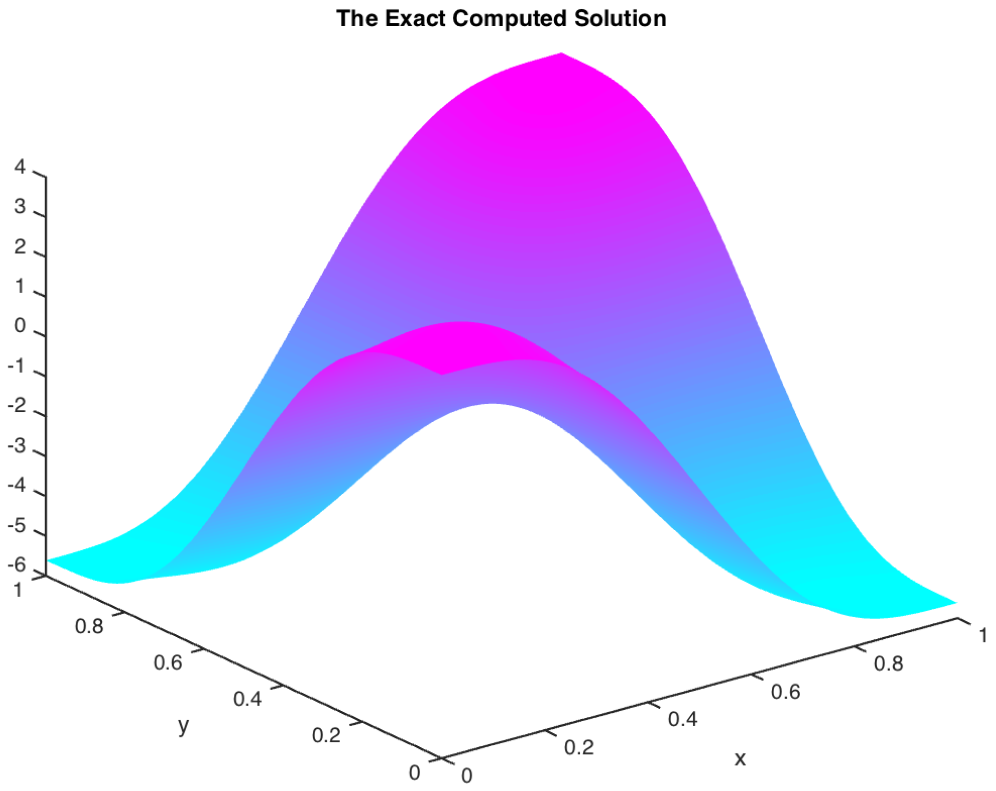
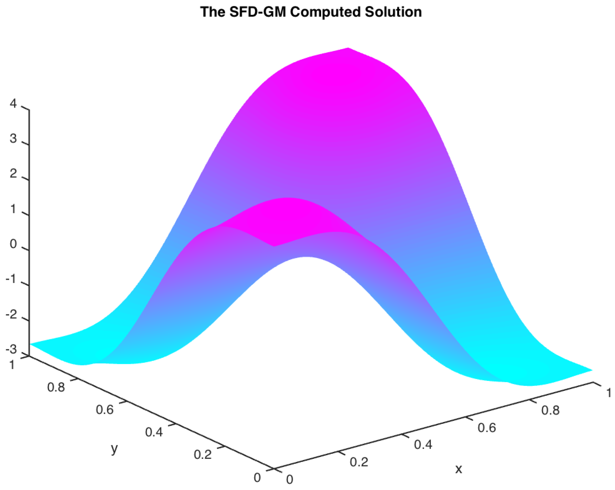
with the prescribed Newton’s iteration, yielding the following Figure 1, Figure 2 and Figure 3. These figures are derived from two experiments, where Figure 2 is the results from the traditional SFD-GM and the second is the results from NSFD-GM discussed earlier. These results are shown in Figure 2 and Figure 3, respectively, and Figure 1 shows the exact solution.

Figure 1.
The exact computed solution.
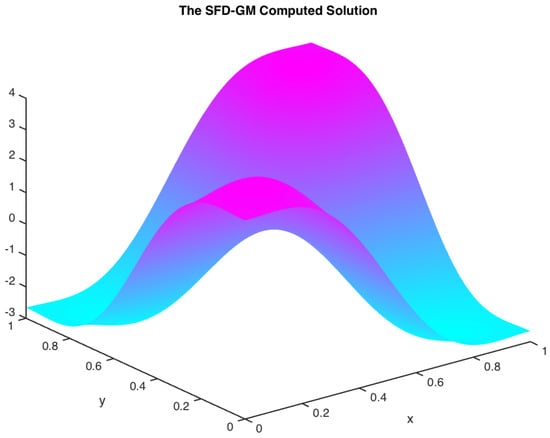
Figure 2.
Approximate solution to the SFD-GM scheme.

Figure 3.
Approximate solution to the NSFD-GM scheme.
With the above illustrated solutions, we fix the space variables and vary the time to obtain the following and errors displayed in the two tables below.
Table 1 displays the errors and the rate of convergence for the NSFD-FEM scheme in both norms, and Table 2 shows the errors and rates of convergence for the SFD-GM scheme also in both norms.

Table 1.
SFD-GM Error in both and -norms.
Table 2.
NSFD-GM Error in both and -norms.
Observations 1.
Using both the NSFD-GM and SFD-GM schemes, we anticipated that the rate of convergence in the -norm will be roughly 2 and that of the -norm will be approximately 1. The rates of convergence in both schemes appear to show some closeness, with the NSFD-GM outperforming the SFD-GM in both and norms according to the results shown in the above tables. These results are expected, since the NSFD-GM scheme consistently demonstrates certain viability and efficiency traits that result from maintaining the qualitative characteristics of the exact solution. Given these additional distinctions, we are forced to support the NSFD-GM scheme.
6. Conclusions and Future Remarks
We started the paper by applying the Galerkin method combined with the compactness method to the Huxley equation. These methods helped us to show theoretically that the continuous solution of the aforementioned equation exists uniquely in the space
with the effect of the parameter well managed. This was followed by designing an efficient scheme NSFD-GM, and we showed that this designed scheme was stable. We proceeded to show that the numerical solution obtained from the designed scheme converges with an optimal rate in both the and the norms. In addition, we showed that the numerical solution preserves all the decaying properties of the exact solution. Furthermore, numerical experiments with the help of an example were conducted to justify the validity of the scheme. All the above processes revealed that the scheme is reliable, accurate and efficient. For this reason, this scheme could act as a fair alternative to the most traditional SFD-GM scheme to solve similar problems such as the Huxley equation.
For further studies, we would like to expand this method to handle real-world problems that involve systems of nonlinear equations connected to the Huxley equation and observe how the parameter affects the solution of the systems. We will also conduct some comparison studies, in terms of efficiency, between the technique presented in this paper and others when applied to problems similar to the one investigated here.
Author Contributions
Conceptualization and formal analysis, P.W.M.C.; writing—review and editing, visualization, C.R.B.M.; project administration, K.R.A. All authors have read and agreed to the published version of the manuscript.
Funding
This research received no external funding.
Data Availability Statement
No data is required for this research.
Acknowledgments
The research contained in this article was supported by Sefako Makgatho Health Sciences University.
Conflicts of Interest
The authors declare no conflict of interest.
References
- Hodgkin, A.; Huxley, A. A quanlitative description of membrane current and its application to conduction and excitation in nerve. J. Physiol. 1952, 117, 500. [Google Scholar] [CrossRef] [PubMed]
- Fitzhugh, R. Impulse and physiological states in theoretical models of nerve membrane. Biophys. J. 1961, 1, 445–466. [Google Scholar] [PubMed]
- Hashim, I.; Noorani, M.S.M.; Batiha, B. A note on the Adomian decomposition method for the generalized Huxley equation. Appl. Math. Comput. 2006, 181, 1439–1445. [Google Scholar] [CrossRef]
- Van der Pol, B.; Van der Mark, J. The heartbeat considered as a relaxation oscillation and an electrical model of the heart. Physiol. Mag. J. Sci. 1928, 6, 763–775. [Google Scholar] [CrossRef]
- Batiha, B.; Noorani, M.S.M.; Hashim, I. Numerical simulation of the generalized Huxley equation by He’s variational iteration method. Appl. Math. Comput. 2007, 186, 1322–1325. [Google Scholar] [CrossRef]
- Wang, X.Y.; Zhu, Z.S.; Lu, Y.K. Solitary wave solutions of the generalized Burger’s-Huxley equation. J. Phys. A Math. Gen. 1990, 23, 271–274. [Google Scholar] [CrossRef]
- Feng, W.J.; Han, X.; Li, Y.S. Fracture analysis for two-dimensional plane problems of nonhomogeneous magneto-electro-thermo-elastic plates subjected to thermal shock by using the meshless local Petrov-Galerkin method. Comput. Model. Eng. Sci. (CMES) 2009, 48, 1. [Google Scholar]
- Lin, J.; Xu, Y.; Reutskiy, S.; Lu, J. A novel Fourier-based meshless method for (3 + 1)-dimensional fractional partial differential equation with general time-dependent boundary conditions. Appl. Math. Lett. 2023, 135, 108441. [Google Scholar] [CrossRef]
- Yang, X.; Zhang, H. The uniform l1 long-time behavior of time discretization for time-fractional partial differential equations with nonsmooth data. Appl. Math. Lett. 2022, 124, 107644. [Google Scholar] [CrossRef]
- Yang, X.; Zhang, H.; Zhang, Q.; Yuan, G.; Sheng, Z. The finite volume scheme preserving maximum principle for two-dimensional time-fractional Fokker–Planck equations on distorted meshes. Appl. Math. Lett. 2019, 97, 99–106. [Google Scholar] [CrossRef]
- Yang, X.; Zhang, H.; Tang, J. The OSC solver for the fourth-order sub-diffusion equation with weakly singular solutions. Comput. Math. Appl. 2021, 82, 1–12. [Google Scholar] [CrossRef]
- Adomian, G. Nonlinera a review of the decomposition method in applied mathematics. J. Math. Anal. Appl. 1988, 135, 501–544. [Google Scholar] [CrossRef]
- Adomian, G. Analytic solution of nonlinear integral equation of Hummerstein type. Appl. Math. Lett. 1998, 11, 127–130. [Google Scholar] [CrossRef]
- Hashemi, S.H.; Daniali, H.R.M.; Ganji, D.D. Numerical simulation of the generalized Huxley equation by He’s homotopy perturbation method. Appl. Math. Comput. 2007, 192, 157–161. [Google Scholar] [CrossRef]
- Sari, M.; Gurarslan, G.; Zeytinoglu, A. High-order finite difference schemes for numerical solutions of the generalized Burger-Huxley equation. Numer. Methods Partial. Differ. Equ. 2010, 27, 1313–1326. [Google Scholar] [CrossRef]
- Chin, P.W.M.; Djoko, J.K.; Lubuma, J.M.-S. Reliable numerical schemes for a linear diffusion equation on a nonsmooth domain. Appl. Math. Lett. 2010, 23, 544–548. [Google Scholar] [CrossRef]
- Zhang, H.; Liu, Y.; Yang, X. An efficient ADI difference scheme for the nonlocal evolution problem in three-dimensional space. J. Appl. Math. Comput. 2023, 69, 651–674. [Google Scholar] [CrossRef]
- Zhou, Z.; Zhang, H.; Yang, X. H1-norm error analysis of a robust ADI method on graded mesh for three-dimensional subdiffusion problems. Numer. Algorithms 2023, 1–19. [Google Scholar] [CrossRef]
- Chin, P.W.M. Optimal Rate of Convergence for a Nonstandard Finite Difference Galerkin Method Applied to Wave Equation Problems. J. Appl. Math. 2013, 2013, 520219. [Google Scholar] [CrossRef]
- Chin, P.W.M. The Galerkin reliable scheme for the numerical analysis of the Burgers’-Fisher equation. Prog. Comput. Fluid Dyn. 2021, 21, 234–247. [Google Scholar] [CrossRef]
- Chin, P.W.M. The study of the numerical treatment of the Real Ginzburg-Landau equation using the Galerkin method. Numer. Funct. Anal. Optim. 2021, 42, 1154–1177. [Google Scholar] [CrossRef]
- Mickens, R.E. Nonstandard Finite Difference Models of Differential Equations; World Scientific: Singapore, 1994. [Google Scholar]
- Anguelov, R.; Lubuma, J.M.-S. Contributions to the mathematics of the nonstandard finite difference method and applications. Numer. Methods Partial. Differ. Equ. 2001, 17, 518–543. [Google Scholar] [CrossRef]
- Anguelov, R.; Lubuma, J.M.-S. Nonstandard finite difference method by nonlocal approximation. Math. Comput. Simul. 2003, 61, 465–475. [Google Scholar] [CrossRef]
- Lubuma, J.M.-S.; Mureithi, E.; Terefe, Y.A. Analysis and dynamically consistent numerical scheme for the SIS model and related reaction diffusion equation. In Application of Mathematics in Technical and Natural Sciences: 3rd International Conference—AMiTaNS’11; AIP Publishing: New York City, NY, USA, 2011; Volume 168. [Google Scholar]
- Lubuma, J.M.-S.; Mureithi, E.W.; Terefe, Y.A. Nonstandard discretization of the SIS Epidemiological model with and without diffusion. Contemp. Math. 2014, 618, 113. [Google Scholar]
- Moghadas, S.M.; Alexander, M.E.; Corbett, B.D.; Gumel, A.B. A positivity-preserving Mickens-type discretization of an epidemic model. J. Differ. Equ. Appl. 2003, 9, 1037–1051. [Google Scholar] [CrossRef]
- Patidar, K.C. On the use of nonstandard finite difference methods. J. Differ. Equ. Appl. 2005, 11, 735–758. [Google Scholar] [CrossRef]
- Appadu, A.R.; Inan, B.; Tijani, Y.O. Comparative study of some numerical methods for the Burgers–Huxley equation. Symmetry 2019, 11, 1333. [Google Scholar] [CrossRef]
- Appadu, A.R.; Tijani, Y.O.; Munyakazi, J. Computational study of some numerical methods for the generalized Burgers-Huxley equation. In Proceedings of the International Conference on Computational Sciences-Modelling, Computing and Software, Singapore, 10–12 September 2020; Springer: Singapore, 2020; pp. 56–67. [Google Scholar]
- Louis, J.L.; Magenes, E.; Kenneth, P. Non-Homogeneous Boundary Value Problems and Applications; Springer: Berlin/Heidelberg, Germany, 1972; Volume 1. [Google Scholar]
- Adams, A.R. Sobolev Space; Academic Press: New York, NY, USA, 1975. [Google Scholar]
- Ciarlet, P.G. The Finite Element Method for Elliptic Problems; Elsevier: Amsterdam, The Netherlands, 1978. [Google Scholar]
- Evan, L.C. Partial Differential Equations. Graduate, Studies in Mathematics; American Mathematical Society: Providence, RI, USA, 1998; Volume 19. [Google Scholar]
- Temam, R. Navier–Stokes Equations: Theory and Numerical Analysis; AMS Chelsea Publishing: Amsterdam, The Netherlands, 1984. [Google Scholar]
- Temam, R. Infinite Dimensional Dynamical System in Mechanics and Physics; Springer: New York, NY, USA, 1997. [Google Scholar]
- Rudin, W. Functional Analysis; McGraw-Hill: New York, NY, USA, 1991. [Google Scholar]
- Aubin, J.P. Un théoréme de compacité. C. R. Acad. Sci. Paris 1963, 256, 5012–5014. [Google Scholar]
- Johnson, C.; Larsson, S.; Thomée, V.; Wahlbin, L.B. Error estimates for spatially discrete approximations of semilinear parabolic equations with nonsmooth initial data. Math. Comput. 1987, 180, 331–357. [Google Scholar] [CrossRef]
- Wheeler, M.F. A priori L2 error estimates for Galerkin approximations to parabolic partial differential equations. SIAM J. Numer. Anal. 1973, 10, 723–759. [Google Scholar] [CrossRef]
- Shen, J. Long time stability and convergence for the fully discrete nonlinear Galerkin methods. Appl. Anal. 1990, 38, 201–229. [Google Scholar] [CrossRef]
- Yang, X.; Zhang, H.; Zhang, Q.; Yuan, G. Simple positivity-preserving nonlinear finite volume scheme for subdiffusion equations on general non-conforming distorted meshes. Nonlinear Dyn. 2022, 108, 3859–3886. [Google Scholar] [CrossRef]
- Yang, X.; Zhang, Z. On conservative, positivity preserving nonlinear FV scheme on distorted meshes for the multi-term nonlocal Nagumo-type equations. Appl. Math. Lett. 2024, 150, 108972. [Google Scholar] [CrossRef]

Disclaimer/Publisher’s Note: The statements, opinions and data contained in all publications are solely those of the individual author(s) and contributor(s) and not of MDPI and/or the editor(s). MDPI and/or the editor(s) disclaim responsibility for any injury to people or property resulting from any ideas, methods, instructions or products referred to in the content. |
© 2024 by the authors. Licensee MDPI, Basel, Switzerland. This article is an open access article distributed under the terms and conditions of the Creative Commons Attribution (CC BY) license (https://creativecommons.org/licenses/by/4.0/).