Improved Bayesian Inferences for Right-Censored Birnbaum–Saunders Data

Abstract

This work focuses on making Bayesian inferences for the two-parameter Birnbaum–Saunders (BS) distribution in the presence of right-censored data. A flexible Gibbs sampler is employed to handle the censored BS data in this Bayesian work that relies on Jeffrey’s and Achcar’s reference priors. A comprehensive simulation study is conducted to compare estimates under various parameter settings, sample sizes, and levels of censoring. Further comparisons are drawn with real-world examples involving Type-II, progressively Type-II, and randomly right-censored data. The study concludes that the suggested Gibbs sampler enhances the accuracy of Bayesian inferences, and both the amount of censoring and the sample size are identified as influential factors in such analyses.

1. Introduction

The Birnbaum–Saunders (BS) distribution is a two-parameter lifetime distribution that was originally introduced by [1] to model the failure time due to the growth of a dominant crack that is subjected to cyclic stress, which causes a failure upon reaching the threshold level. The BS distribution has gone through various developments and generalizations and is found to be suitable for life testing applications. The distribution was originally derived to model the fatigue life of metals that are subject to periodic stress; this is sometimes referred to as the fatigue life distribution. Interestingly, it can also be obtained by using a monotone transformation on the standard normal distribution [2]. Moreover, as [3] indicated, the BS distribution can be viewed as an equal mixture of an inverse Gaussian (IG) distribution and its reciprocal. These relations are useful in deriving important properties of the BS distribution based on well-known properties of the normal and IG distributions. Ref. [4] showed that the BS distribution can be used as an approximation of the IG distribution. In practice, both the BS and IG distributions are often considered very competitive lifetime models for right-skewed data [5,6].

The distribution function of the BS failure time T with parameters $\alpha$ and $\beta$, denoted by $T\sim BS(\alpha ,\beta )$, is given by

$$F_T\left(t\right)=\Phi \left[\frac{1}{\alpha }\left(\sqrt{\frac{t}{\beta }}-\sqrt{\frac{\beta }{t}}\right)\right],$$

(1)

where $0<t<\infty ,$ and $\alpha >0,\beta >0$ are the shape and scale parameters, respectively. Here, $\Phi (·)$ represents the distribution function of the standard normal distribution. Since $F_T\left(\beta \right)=\Phi \left(0\right)=0.5$, the scale parameter $\beta$ is the median of the BS distribution. The probability density function (pdf) of the $BS(\alpha ,\beta )$ is given by

$$f_T\left(t\right)=\frac{1}{2\sqrt{2\pi }\alpha \beta }\left[{\left(\frac{\beta }{t}\right)}^{1/2}+{\left(\frac{\beta }{t}\right)}^{3/2}\right]exp\left[-\frac{1}{2{\alpha }^2}\left(\frac{t}{\beta }+\frac{\beta }{t}-2\right)\right]$$

(2)

It can be easily shown that $E\left(T\right)=\beta (1+{\alpha }^2/2)$ and $Var\left(T\right)={\left(\alpha \beta \right)}^2(1+5{\alpha }^2/4)$. Interestingly, Ref. [7] indicates that $T^{-1}\sim BS(\alpha ,{\beta }^{-1})$, and therefore the reciprocal variable $T^{-1}$ also belongs to the same family.

The parameter estimation for the BS distribution, including the maximum likelihood estimation (MLE), is largely discussed in its literature. For complete data, Ref. [8] derived the MLE’s of the BS parameters. Ref. [9] introduced modified moment estimators (MMEs), a bias reduction method and a Jackknife technique to reduce the bias of both MMEs and MLEs. Ref. [10] introduced alternative estimators with a smaller bias compared to that for Ref. [9]. Point and interval estimations of the BS parameters under Type-II censoring are discussed in [11]. Ref. [12] suggested a modified censored moment estimation method to estimate its parameters under random censoring. Ref. [13] suggested using a fiducial inference on BS parameters for right-censored data.

Bayesian approaches have also been used to make inferences on the BS parameters. Ref. [14] used both Jeffrey’s prior and a reference prior to derive marginal posteriors using Laplace’s approximation; while [15] employed only the reference priors and considered an approximate Bayesian approach using Lindley’s method. Ref. [16] justified that Jeffrey’s reference prior results in an improper posterior for the scale parameter and suggested employing the reference priors that incorporate some partial information. In this situation, they suggested applying the slice sampling method to obtain a proper posterior for the case of censored data. A work by [17] adopted inverse-gamma priors for the shape and scale parameters and proposed an efficient sampling algorithm using the generalized ratio-of-uniforms method to compute Bayesian estimates. Ref. [18] also adapted the inverse-gamma priors for both the BS parameters and applied Markov Chain Monte Carlo (MCMC)-based conditional and joint sampling methods to handle censored data.

The censored data appear in life-time experiments due to various reasons; the nature of censoring plays a vital role in its analysis. In this study, we focus on the right-censored data that occurs when the test start time of each unit is known, but the test end time is unknown. This includes the random right, Type-II, and progressively Type-II censoring schemes. The progressively Type-II censoring scheme allows one to remove a pre-specified number of uncensored units from the remaining experimental units at the observed failure times [19]. As such, it is a more general form of Type-II censoring, where censoring takes place progressively in r stages. In this scheme, a total of n units are placed on a life-test, only r are completely observed until failure and the rest of $n-r$ units are rightly censored. However, at the time of the first failure, say $t_{\left(1\right)}$, $R_1$ of the $n-1$ surviving units are randomly withdrawn from the experiment; at the time of the next failure, say $t_{\left(2\right)}$, $R_2$ of the $n-2-R_1$ surviving units are censored, and so on. At the time of the last (rth) failure, say $t_{\left(r\right)}$, all the remaining $R_r=n-r-{\sum }_{j=1}^{r-1}{R}_j$ surviving units are censored. Therefore, in progressively Type-II censoring experiments with pre-specified r and $\{R_1,R_2,\dots ,R_r\}$, the data will take the form $\{(t_{\left(1\right)},R_1),(t_{\left(2\right)},R_2),\dots ,(t_{\left(r\right)},R_r)\}$.

In this work, we focus on estimating both BS parameters in the presence of right-censored units as well as the average remaining test time $\overline{T}$ of the censored units. For instance, let us consider n non-repairable units and assume we observe failures in r progressively censored stages with censored times ${\mathbf{y}}^{\prime }=(t_{\left(1\right)},t_{\left(2\right)},\dots ,t_{\left(r\right)})$. If the experiment were to continue so that all $(n-r)$ -censored values could be observed, then we let ${\tilde{\mathbf{y}}}_i^{\prime }=(t_{(i:1)},t_{(i:2)},\dots ,t_{(i:R_i)})$ be the set of true observed values of the censored values at the ith progressive stage. Then, the remaining total test time for these $R_i$ censored elements is ${\tilde{\mathbf{y}}}_i^{\prime }{\displaystyle 1}-t_{\left(i\right)}{{\displaystyle 1}}^{\prime }{\displaystyle 1}$, where 1 is a column vector of 1’s of length $R_i$. As such, the estimated and average remaining test time for all the censored units from all r progressive stages is

$$\overline{T}=\frac{1}{n-r}\sum _{i=1}^r\left({\tilde{\mathbf{y}}}_i^{\prime }{\displaystyle 1}-t_{\left(i\right)}{{\displaystyle 1}}^{\prime }{\displaystyle 1}\right).$$

(3)

The rest of the article is organized as follows: In Section 2, we discuss the parameter estimation of the BS distribution using both the maximum likelihood method and the Bayesian method. Section 3 covers the Gibbs sampling procedure for handling censored data. In Section 4, we conduct a Monte–Carlo simulation study to compare the performance of the aforementioned methods. Illustrative examples are included in Section 5, and we conclude with remarks and recommendations in Section 6.

2. BS Parameter Estimation

In this section, we focus on the Bayesian parameter estimation with two different prior specifications: Jeffrey’s and Achcar’s priors for the BS parameters $\alpha$ and $\beta$. We discuss some of the practical challenges of these procedures while summarizing their methodological foundations.

On the other hand, the MLE of BS parameters, $\alpha$ and $\beta$, were heavily discussed in the literature; see [2,8] for details. Consider an experiment with n random failure times $\mathbf{T}$ = {$t_1,t_2,\dots ,t_n$} that follow the BS distribution. Then, its log-likelihood function, without the additive constant, becomes

$$l(\alpha ,\beta |\mathbf{T})=-nln\left(\alpha \beta \right)+\sum _{i=1}^{n}ln\left[{\left(\frac{\beta }{t_i}\right)}^{1/2}+{\left(\frac{\beta }{t_i}\right)}^{3/2}\right]-\frac{1}{2{\alpha }^2}\sum _{i=1}^n\left(\frac{t_i}{\beta }+\frac{\beta }{t_i}-2\right).$$

(4)

By differentiating Equation (4) with respect to $\alpha$ and solving it for zero, one can obtain

$${\alpha }^2=\left[\frac{s}{\beta }+\frac{\beta }{q}-2\right],$$

(5)

where $s={\sum }_{i=1}^n{t}_i/n$ and $q={\left[{\sum }_{i=1}^n{t}_i^{-1}/n\right]}^{-1}$ are the sample arithmetic and harmonic means of the observed data. Next, when differentiating Equation (4) with respect to $\beta$ and substituting ${\alpha }^2$ from Equation (5), the following can be obtained to determine the MLE of $\beta$.

$${\beta }^2-\beta (2q+K\left(\beta \right))+q(s+K\left(\beta \right))=0,$$

(6)

where $K\left(\beta \right)={\left[{\sum }_{i=1}^n{(\beta +t_i)}^{-1}/n\right]}^{-1}$. The MLE $\widehat{\beta }$ of $\beta$ is the unique positive root of Equation (6), in which $q<\widehat{\beta }<s$. With this estimate, the MLE of $\alpha$ becomes $\widehat{\alpha }={\left[\frac{s}{\widehat{\beta }}+\frac{\widehat{\beta }}{q}-2\right]}^{1/2}$.

2.1. Bayesian Inference

Here, we consider the Bayesian work that was originally suggested by [14] by employing non-informative priors that include Jeffrey’s and Achcar’s reference priors. Jeffrey’s prior density for $\alpha$ and $\beta$ is given by

$$\pi (\alpha ,\beta )\propto \sqrt{\det \mathit{I}(\alpha ,\beta )},$$

where $\mathit{I}(\alpha ,\beta )=\left(\begin{array}{cc}\frac{2n}{{\alpha }^2}& 0\\ 0& \frac{n[1+\alpha g\left(\alpha \right)/\sqrt{2\pi }]}{{\alpha }^2{\beta }^2}\end{array}\right)$ is the Fisher information matrix of the BS distribution, $g\left(\alpha \right)=\alpha \sqrt{\pi /2}-\pi exp\{2/{\alpha }^2\}[1-\Phi (2/\alpha )]$, and $\Phi$ is the standard normal distribution function.

Using the Laplace approximation, it can be shown that Jeffrey’s prior takes the following form

$$\pi (\alpha ,\beta )\propto \frac{1}{\alpha \beta }H\left({\alpha }^2\right),\alpha >0,\beta >0,$$

where $H\left({\alpha }^2\right)=\left(\frac{1}{{\alpha }^2}+\frac{1}{4}\right)$.

Assuming independence between $\alpha$ and $\beta$, [14] suggested a reference prior that takes the following form

$$\pi (\alpha ,\beta )\propto \frac{1}{\alpha \beta },\alpha >0,\beta >0.$$

In our discussion, we called this Achcar’s reference prior.

2.2. Posterior Inference

For Jeffrey’s prior, the joint posterior distribution of $\alpha$ and $\beta$ becomes [14]

$$\pi (\alpha ,\beta |\mathbf{T})\propto \frac{{\prod }_{i=1}^n(\beta +t_i)exp\{-Q\left(\beta \right)/{\alpha }^2\}}{{\alpha }^{n+1}{\beta }^{(n/2)+1}H\left({\alpha }^2\right)},$$

(7)

where $Q\left(\beta \right)=\frac{ns}{2\beta }+\frac{n\beta }{2q}-n$.

Then, using the Laplace approximation (see Appendix A), the approximate marginal posterior distributions of $\alpha$ and $\beta$ for Jeffrey’s prior can be written as

$$\pi \left(\alpha \right|\mathbf{T})\propto {\alpha }^{-(n+1)}{(4+{\alpha }^2)}^{1/2}exp\left\{-\frac{n}{{\alpha }^2}(\sqrt{s/q}-1)\right\},\alpha >0,$$

(8)

and

$$\pi \left(\beta \right|\mathbf{T})\propto \frac{{\prod }_{i=1}^n(\beta +t_i){\left\{4+[2n/(n+2\left)\right][s/(2\beta )+\beta /(2q)-1]\right\}}^{1/2}}{{\beta }^{(n/2)+1}{\left\{s/\left(2\beta \right)+\beta /\left(2q\right)-1\right\}}^{(n+1)/2}},\beta >0,$$

(9)

respectively.

Then, for Achcar’s reference prior, the joint posterior becomes the same as Equation (7) except where $H\left({\alpha }^2\right)=1$ and the approximate marginal posterior distributions of $\alpha$ and $\beta$ become

$$\pi \left(\alpha \right|\mathbf{T})\propto {\alpha }^{-n}exp\left\{-\frac{n}{{\alpha }^2}(\sqrt{s/q}-1)\right\},\alpha >0,$$

(10)

and

$$\pi \left(\beta \right|\mathbf{T})\propto \frac{{\prod }_{i=1}^n(\beta +t_i)}{{\beta }^{(n/2)+1}{\left\{s/\left(2\beta \right)+\beta /\left(2q\right)-1\right\}}^{n/2}},\beta >0,$$

(11)

respectively.

As both Jeffrey- and Achcar-based posteriors do not have closed-form distributions, the Bayes estimates of $\alpha$ and $\beta$ cannot be obtained in an explicit form. However, [14] proposed that the mode of the corresponding posteriors may be used as the Bayes estimates for $\alpha$ and $\beta$.

The work by [16] has shown that the above Achcar’s reference prior based posterior given in Equation (11) becomes improper when $\beta \to \infty$. In practice, both posteriors given in Equations (9) and (11) are numerically intractable for larger $\beta$ and n values due to the increments of the products in their numerators. However, as $F_T(t,\alpha ,\beta )=F_T(t/\beta ,\alpha ,1)$, the parameter $\beta$ in the BS distribution is solely a scale parameter which represents the median. Therefore, we suggest a simple and computationally efficient scaler transformation $t_{new}=t/\widehat{\beta }$ to reduce this inflation and to avoid the situation that $\beta \to \infty$. As a result, the median of the transformed data and the posteriors of $\beta$ will be centered around one.

3. Application of Gibbs Sampler

In this section, we introduce a Gibbs sampling procedure that can be used to estimate the parameters of the BS distribution in the presence of censored data. The procedure uses Markov Chain Monte Carlo (MCMC) techniques to generate data samples that replace the censored portion of the data set.

Here, we propose using Bayesian inference for BS parameters $\alpha$ and $\beta$, employing marginal posteriors obtained using both Jeffrey’s and Achcar’s priors via the Gibbs sampler. Moreover, upon sampling from a BS distribution for unknown realizations of censored units, the remaining average lifetime is also estimated.

The Gibbs sampler requires suitable initial values for $\alpha$ and $\beta$ to achieve its convergence. Often the MLE’s from the observed data given censoring are preferred for this purpose. Ignoring the additive constant, the BS log-likelihood function for the progressively Type-II-censored data of the form $\{(t_{\left(1\right)},R_1),(t_{\left(2\right)},R_2),\dots ,(t_{\left(r\right)},R_r)\}$ can be written as

$$l(\alpha ,\beta |\mathbf{T})=\sum _{i=1}^r\left\{lnf(t_{\left(i\right)};\alpha ,\beta )+R_{i}ln(\Phi (-g(t_{\left(i\right)};\alpha ,\beta )))\right\},$$

(12)

where $f(·)$ is the pdf of the BS distribution given in Equation (2), and $g(t;\alpha ,\beta )=\frac{1}{\alpha }\left(\sqrt{\frac{t}{\beta }}-\sqrt{\frac{\beta }{t}}\right)$.

The MLEs of the BS parameters cannot be obtained in the closed form for this censoring scheme. Using the property that the BS distribution can be written as an equal mixture of an IG distribution and its reciprocal [20] outlined an EM algorithm to obtained its MLEs. In this work, we use a computational tool introduced in [21] that is freely available in [22], which can be used to obtain MLEs of the BS parameters with all major censoring schemes.

Below, we outline the major steps of the Gibbs sampler, which employs progressively Type-II-censored BS data.

• Calculate the MLE ${\widehat{\alpha }}_{MLE}$ and ${\widehat{\beta }}_{MLE}$ from the available right-censored data. Set ${\widehat{\alpha }}_{MLE}={\alpha }_1^{\left(0\right)}$ and ${\widehat{\beta }}_{MLE}={\beta }_1^{\left(0\right)}$.
• Generate $R_i$ random variates from a uniform distribution bounded by the BS CDF $\left(F_T\right)$ value of the respective censored observation and one. Then, use the inverse CDF ($F_T^{-1}$) value of the newly sampled random variate to replace the censored value. For instance, for the jth censored observation in $(t_{\left(i\right)},R_i)$,
  • Generate: $u_{(j:i)}\sim U\left[F_T\left(t_{\left(i\right)}\right),1\right]$, where $F_T\left(t_{\left(i\right)}\right)=\Phi \left[\frac{1}{{\alpha }_1^{\left(0\right)}}\left(\sqrt{\frac{t_{\left(i\right)}}{{\beta }_1^{\left(0\right)}}}-\sqrt{\frac{{\beta }_1^{\left(0\right)}}{t_{\left(i\right)}}}\right)\right]$.
  • Then, set: $t_{(j:i)}^{\left(0\right)}=F_T^{-1}\left(u_{(j:i)};{\alpha }_1^{\left(0\right)},{\beta }_1^{\left(0\right)}\right)$.
• Repeat Step 2 for all censored units in all r censored stages. The censored data will be replaced by the the newly simulated data $t_{(j:i)}^{\left(0\right)}$ ($>t_{\left(i\right)}$), $\forall j=1,2,\dots ,R_i$ for each $i=1,2,\dots ,r$ and will be combined with the observed failure times $t_{\left(1\right)},t_{\left(2\right)},\dots ,t_{\left(r\right)}$ to form an updated and complete sample of size n.
• Using the updated sample in Step 3, sample ${\alpha }_1^{\left(1\right)}$ and ${\beta }_1^{\left(1\right)}$ from their respective posterior distributions.
• Repeat Steps 2–4 starting with the newly sampled parameters, ${\alpha }_1^{\left(1\right)}$ and ${\beta }_1^{\left(1\right)}$. This procedure will continue for k total iterations and conclude with the results for ${\alpha }_1^{\left(k\right)}$ and ${\beta }_1^{\left(k\right)}$. A new set of simulated BS observations should be picked in the same manner as in Step 3 using the ${\alpha }_1^{\left(k\right)}$ and ${\beta }_1^{\left(k\right)}$ as newly updated parameters.
• At the conclusion of Step 5, the average remaining life of censored units defined in Equation (3) shall be calculated using the newly sampled data and is designated as ${\overline{T}}_1^{\left(k\right)}$.
• Repeat the above process in Step 2–6 a large number of times, say m total replications. This will result:

  $$({\alpha }_1^{\left(k\right)},{\alpha }_2^{\left(k\right)},\dots ,{\alpha }_m^{\left(k\right)}),({\beta }_1^{\left(k\right)},{\beta }_2^{\left(k\right)},\dots ,{\beta }_m^{\left(k\right)}),({\overline{T}}_1^{\left(k\right)},{\overline{T}}_2^{\left(k\right)},\dots ,{\overline{T}}_m^{\left(k\right)}).$$

In the Gibbs sampler, we guarantee the convergence of the sampled data using both numerical and graphical summaries. This includes monitoring the scalar summary $\psi$ and the scale reduction statistic $\widehat{R}$ defined in [23]. As suggested in [24], we confirm that this scale reduction statistic is well below 1.1 and the trace plots behave appropriately to ensure the convergence of the Gibbs samples in all situations considered. After confirming the convergence, we report both point and interval estimates. This includes mean and its stand error estimates as well as the 95% equal-tailed credible intervals for all the parameters including $\overline{T}$. Moreover, we use the Kernel density estimation procedure to make visual comparisons between estimation methods. A sample R code to exhibit this algorithm is included in the Supplementary Materials.

4. Monte–Carlo Simulation

We conduct a simulation study to compare the performance of the discussed Bayesian estimates. The data are generated from the $BS(\alpha ,\beta )$ distribution with four different sample sizes $n=10,20,30,50$ and four different Type-II right-censoring percentages (CEP) at 10%(10%)40%. Without a loss of generality, we kept the scale parameter $\beta$ fixed at 1.0 while varying the shape parameter $\alpha =0.10,0.30,0.50,1.00,2.00$. In each experimental condition, we repeatedly generated 2000 BS data sets and applied the proposed Gibbs sampler.

We noticed that the Gibbs sampler converges in $k=3000$ iterations for both Bayesian priors, and the scale reduction factor $\widehat{R}$ for both parameters is less than 1.1. After assessing the convergence, we replicate the Gibbs sampler $m=1000$ times to obtain the point and 95% equal-tailed credible intervals for $\alpha$, $\beta$, and $\overline{T}$ for each generated data set. Then for each parameter, the overall average of the posterior mean estimates (PE), its standard error (SE), and the coverage probability (CP) for 1000 randomly generated BS samples are acquired. To compare posterior point estimates, we refer to an observed bias as the difference between the true BS parameter and its PE. These results are shown in Table 1, Table 2, Table 3 and Table 4.

Table 1. Mean and standard error of the point estimates and probability coverages of 95% credible intervals based on Monte–Carlo simulation ($n=10$).

		$\widehat{\mathit{\alpha }}$						$\widehat{\mathit{\beta }}$						$\widehat{\overline{\mathit{T}}}$
Param	CEP%	Jeffrey’s			Achcar’s			Jeffrey’s			Achcar’s			Jeffrey’s			Achcar’s
$\mathbf{\alpha }$		PE	SE	CP	PE	SE	CP	PE	SE	CP	PE	SE	CP	PE	SE	CP	PE	SE	CP
0.1	10	0.100	0.025	0.939	0.108	0.027	0.957	1.003	0.034	0.927	1.001	0.031	0.952	0.063	0.019	0.940	0.071	0.021	0.942
	20	0.101	0.029	0.942	0.110	0.030	0.949	1.002	0.033	0.932	1.001	0.032	0.955	0.072	0.024	0.936	0.080	0.027	0.940
	30	0.101	0.031	0.934	0.113	0.035	0.956	1.002	0.033	0.916	1.006	0.034	0.951	0.078	0.028	0.925	0.091	0.033	0.954
	40	0.099	0.035	0.922	0.112	0.036	0.965	1.002	0.037	0.920	1.007	0.038	0.945	0.085	0.034	0.921	0.101	0.039	0.951
0.3	10	0.299	0.074	0.933	0.316	0.075	0.953	1.013	0.099	0.933	1.008	0.097	0.949	0.256	0.091	0.946	0.280	0.096	0.941
	20	0.293	0.079	0.932	0.319	0.082	0.960	1.008	0.099	0.931	1.014	0.100	0.947	0.265	0.102	0.928	0.301	0.108	0.943
	30	0.289	0.083	0.933	0.317	0.088	0.959	1.007	0.101	0.928	1.020	0.104	0.944	0.277	0.110	0.944	0.319	0.122	0.948
	40	0.289	0.091	0.918	0.320	0.094	0.952	1.013	0.110	0.922	1.026	0.117	0.938	0.297	0.125	0.923	0.346	0.137	0.944
0.5	10	0.489	0.115	0.938	0.517	0.123	0.945	1.032	0.159	0.941	1.026	0.166	0.936	0.543	0.218	0.940	0.592	0.244	0.951
	20	0.487	0.124	0.937	0.523	0.121	0.962	1.033	0.162	0.938	1.038	0.171	0.949	0.559	0.236	0.938	0.617	0.234	0.960
	30	0.475	0.125	0.949	0.515	0.128	0.960	1.025	0.172	0.927	1.046	0.168	0.950	0.552	0.235	0.942	0.629	0.247	0.945
	40	0.466	0.141	0.930	0.509	0.132	0.973	1.018	0.175	0.920	1.039	0.187	0.951	0.562	0.266	0.934	0.638	0.266	0.961
1	10	1.002	0.261	0.939	1.056	0.260	0.953	1.088	0.306	0.936	1.085	0.297	0.959	1.849	1.058	0.938	1.929	1.021	0.946
	20	1.002	0.289	0.924	1.073	0.291	0.947	1.085	0.307	0.943	1.104	0.304	0.961	1.899	1.188	0.948	2.072	1.180	0.940
	30	1.000	0.315	0.929	1.062	0.314	0.953	1.089	0.319	0.931	1.108	0.320	0.951	1.917	1.235	0.928	2.053	1.238	0.939
	40	0.983	0.337	0.930	1.079	0.344	0.957	1.067	0.318	0.922	1.116	0.328	0.956	1.873	1.246	0.929	2.141	1.339	0.961
2	10	1.961	0.465	0.946	2.013	0.473	0.948	1.111	0.416	0.954	1.109	0.420	0.965	6.634	4.577	0.918	6.923	4.658	0.917
	20	1.944	0.519	0.924	2.014	0.512	0.938	1.098	0.420	0.945	1.103	0.419	0.962	6.186	4.583	0.904	6.172	4.344	0.923
	30	1.868	0.545	0.927	1.943	0.541	0.938	1.065	0.425	0.949	1.103	0.433	0.957	5.193	3.955	0.921	5.529	4.439	0.922
	40	1.755	0.588	0.904	1.898	0.522	0.957	1.022	0.434	0.912	1.059	0.437	0.954	4.437	3.616	0.876	4.833	3.530	0.934

Table 2. Mean and standard error of the point estimates and probability coverages of 95% credible intervals based on Monte–Carlo simulation ($n=20$).

		$\widehat{\mathit{\alpha }}$						$\widehat{\mathit{\beta }}$						$\widehat{\overline{\mathit{T}}}$
Param	CEP%	Jeffrey’s			Achcar’s			Jeffrey’s			Achcar’s			Jeffrey’s			Achcar’s
$\mathbf{\alpha }$		PE	SE	CP	PE	SE	CP	PE	SE	CP	PE	SE	CP	PE	SE	CP	PE	SE	CP
0.1	10	0.099	0.018	0.939	0.103	0.018	0.943	0.999	0.022	0.943	1.002	0.023	0.944	0.059	0.013	0.947	0.062	0.013	0.938
	20	0.100	0.019	0.936	0.104	0.020	0.951	1.000	0.023	0.940	1.002	0.024	0.944	0.066	0.015	0.937	0.071	0.016	0.951
	30	0.099	0.022	0.933	0.104	0.022	0.963	0.999	0.024	0.945	1.001	0.024	0.937	0.073	0.018	0.929	0.078	0.019	0.950
	40	0.100	0.024	0.936	0.105	0.025	0.957	1.000	0.025	0.934	1.003	0.026	0.945	0.081	0.022	0.929	0.087	0.023	0.946
0.3	10	0.302	0.054	0.944	0.310	0.054	0.950	1.004	0.066	0.939	1.007	0.068	0.949	0.245	0.066	0.954	0.257	0.068	0.954
	20	0.303	0.059	0.937	0.313	0.060	0.954	1.006	0.070	0.938	1.005	0.069	0.948	0.263	0.075	0.944	0.277	0.078	0.953
	30	0.299	0.062	0.946	0.308	0.064	0.948	1.006	0.071	0.938	1.010	0.076	0.934	0.274	0.081	0.944	0.288	0.086	0.949
	40	0.299	0.069	0.945	0.322	0.070	0.953	1.002	0.076	0.935	1.015	0.080	0.949	0.291	0.093	0.935	0.325	0.099	0.957
0.5	10	0.504	0.089	0.938	0.522	0.088	0.959	1.016	0.116	0.935	1.018	0.113	0.948	0.540	0.170	0.961	0.571	0.170	0.959
	20	0.499	0.096	0.937	0.513	0.093	0.953	1.019	0.114	0.954	1.020	0.115	0.939	0.548	0.179	0.945	0.573	0.179	0.959
	30	0.494	0.100	0.940	0.509	0.096	0.961	1.019	0.122	0.937	1.020	0.124	0.939	0.556	0.192	0.937	0.582	0.189	0.952
	40	0.501	0.110	0.941	0.519	0.111	0.951	1.017	0.125	0.952	1.029	0.136	0.945	0.586	0.212	0.945	0.625	0.222	0.962
1	10	0.998	0.177	0.947	1.029	0.182	0.947	1.049	0.218	0.942	1.050	0.220	0.951	1.841	0.745	0.948	1.956	0.798	0.954
	20	1.003	0.200	0.939	1.038	0.208	0.939	1.052	0.220	0.950	1.073	0.236	0.955	1.847	0.844	0.938	2.002	0.963	0.948
	30	1.004	0.218	0.942	1.051	0.234	0.943	1.051	0.230	0.945	1.070	0.255	0.951	1.843	0.917	0.945	2.054	1.129	0.957
	40	1.008	0.248	0.952	1.063	0.265	0.941	1.070	0.259	0.953	1.093	0.264	0.958	1.933	1.138	0.951	2.155	1.236	0.946
2	10	2.021	0.364	0.935	2.055	0.361	0.942	1.103	0.328	0.952	1.106	0.329	0.957	7.592	3.552	0.945	7.841	3.705	0.955
	20	1.988	0.395	0.928	2.025	0.374	0.951	1.103	0.360	0.934	1.118	0.365	0.943	7.070	3.777	0.944	7.367	3.807	0.951
	30	1.972	0.425	0.953	2.032	0.412	0.957	1.101	0.358	0.955	1.122	0.369	0.959	6.813	3.815	0.949	7.250	3.888	0.946
	40	1.997	0.458	0.950	2.046	0.443	0.966	1.106	0.381	0.953	1.136	0.376	0.963	6.844	4.108	0.957	7.219	3.982	0.963

Table 3. Mean and standard error of the point estimates and probability coverages of 95% credible intervals based on Monte–Carlo simulation ($n=30$).

		$\widehat{\mathit{\alpha }}$						$\widehat{\mathit{\beta }}$						$\widehat{\overline{\mathit{T}}}$
Param	CEP%	Jeffrey’s			Achcar’s			Jeffrey’s			Achcar’s			Jeffrey’s			Achcar’s
$\mathbf{\alpha }$		PE	SE	CP	PE	SE	CP	PE	SE	CP	PE	SE	CP	PE	SE	CP	PE	SE	CP
0.1	10	0.099	0.014	0.943	0.101	0.014	0.956	1.000	0.018	0.946	0.999	0.019	0.938	0.058	0.010	0.949	0.060	0.010	0.954
	20	0.101	0.015	0.952	0.102	0.015	0.948	1.000	0.019	0.947	1.001	0.019	0.936	0.066	0.012	0.950	0.068	0.012	0.951
	30	0.100	0.017	0.937	0.103	0.018	0.939	1.001	0.020	0.938	1.000	0.020	0.955	0.073	0.015	0.953	0.076	0.015	0.949
	40	0.100	0.020	0.933	0.103	0.019	0.955	1.000	0.021	0.932	1.001	0.020	0.958	0.080	0.018	0.925	0.083	0.017	0.963
0.3	10	0.301	0.043	0.948	0.306	0.042	0.956	1.006	0.056	0.940	1.003	0.055	0.943	0.239	0.052	0.943	0.245	0.052	0.940
	20	0.298	0.046	0.941	0.308	0.047	0.957	1.001	0.056	0.940	1.005	0.057	0.957	0.251	0.057	0.940	0.265	0.059	0.956
	30	0.300	0.051	0.926	0.309	0.053	0.952	1.003	0.060	0.944	1.004	0.060	0.948	0.269	0.066	0.945	0.282	0.068	0.960
	40	0.295	0.057	0.933	0.311	0.058	0.949	1.002	0.061	0.938	1.006	0.062	0.959	0.281	0.075	0.934	0.302	0.081	0.947
0.5	10	0.502	0.069	0.956	0.506	0.075	0.938	1.013	0.093	0.946	1.010	0.096	0.934	0.526	0.128	0.948	0.533	0.142	0.935
	20	0.502	0.075	0.952	0.513	0.084	0.932	1.010	0.093	0.951	1.013	0.095	0.948	0.537	0.140	0.952	0.560	0.159	0.932
	30	0.500	0.086	0.935	0.518	0.086	0.947	1.012	0.098	0.938	1.017	0.098	0.956	0.552	0.162	0.948	0.583	0.165	0.954
	40	0.502	0.094	0.946	0.517	0.092	0.962	1.015	0.106	0.937	1.015	0.104	0.955	0.574	0.177	0.925	0.599	0.179	0.962
1	10	0.994	0.145	0.945	1.024	0.149	0.956	1.038	0.175	0.952	1.042	0.180	0.937	1.785	0.593	0.942	1.895	0.660	0.936
	20	1.004	0.162	0.935	1.030	0.161	0.948	1.028	0.181	0.943	1.037	0.181	0.954	1.755	0.650	0.951	1.850	0.668	0.946
	30	1.002	0.179	0.946	1.024	0.186	0.938	1.040	0.205	0.937	1.053	0.200	0.945	1.755	0.763	0.945	1.840	0.781	0.953
	40	1.005	0.210	0.938	1.043	0.211	0.951	1.049	0.216	0.945	1.075	0.232	0.944	1.799	0.921	0.940	1.954	0.973	0.949
2	10	2.010	0.301	0.933	2.027	0.295	0.941	1.074	0.286	0.939	1.075	0.267	0.958	7.219	2.993	0.946	7.284	2.882	0.949
	20	2.008	0.324	0.945	2.024	0.336	0.929	1.078	0.299	0.937	1.066	0.295	0.943	6.914	3.202	0.948	6.970	3.344	0.937
	30	2.028	0.373	0.947	2.052	0.374	0.946	1.114	0.339	0.934	1.117	0.325	0.953	7.069	3.779	0.951	7.232	3.739	0.936
	40	1.996	0.411	0.943	2.053	0.409	0.953	1.101	0.347	0.959	1.148	0.355	0.962	6.656	3.848	0.941	7.221	4.098	0.955

Table 4. Mean and standard error of the point estimates and probability coverages of 95% credible intervals based on Monte–Carlo simulation ($n=50$).

		$\widehat{\mathit{\alpha }}$						$\widehat{\mathit{\beta }}$						$\widehat{\overline{\mathit{T}}}$
Param	CEP%	Jeffrey’s			Achcar’s			Jeffrey’s			Achcar’s			Jeffrey’s			Achcar’s
$\mathbf{\alpha }$		PE	SE	CP	PE	SE	CP	PE	SE	CP	PE	SE	CP	PE	SE	CP	PE	SE	CP
0.1	10	0.100	0.011	0.950	0.101	0.011	0.949	1.000	0.014	0.945	0.999	0.014	0.958	0.057	0.007	0.950	0.058	0.008	0.944
	20	0.100	0.012	0.935	0.101	0.012	0.941	0.999	0.014	0.942	1.000	0.015	0.943	0.065	0.009	0.947	0.066	0.009	0.945
	30	0.100	0.013	0.934	0.102	0.013	0.953	1.000	0.015	0.940	1.000	0.016	0.936	0.072	0.011	0.935	0.073	0.011	0.932
	40	0.099	0.014	0.945	0.102	0.015	0.945	1.000	0.016	0.939	1.000	0.016	0.952	0.078	0.013	0.944	0.081	0.013	0.938
0.3	10	0.302	0.033	0.946	0.304	0.033	0.948	1.003	0.042	0.945	1.003	0.042	0.949	0.236	0.039	0.950	0.239	0.039	0.935
	20	0.299	0.035	0.952	0.306	0.034	0.954	1.003	0.045	0.928	1.000	0.042	0.949	0.249	0.043	0.945	0.256	0.042	0.952
	30	0.298	0.039	0.942	0.305	0.041	0.949	1.002	0.046	0.941	1.002	0.044	0.951	0.263	0.049	0.946	0.272	0.051	0.942
	40	0.301	0.045	0.930	0.306	0.045	0.945	1.004	0.049	0.944	1.002	0.049	0.947	0.282	0.059	0.946	0.289	0.060	0.939
0.5	10	0.500	0.056	0.943	0.506	0.055	0.946	1.004	0.071	0.937	1.007	0.069	0.959	0.511	0.103	0.954	0.522	0.103	0.933
	20	0.502	0.057	0.967	0.504	0.059	0.950	1.004	0.072	0.939	1.007	0.074	0.942	0.527	0.107	0.949	0.532	0.111	0.944
	30	0.500	0.067	0.944	0.507	0.067	0.942	1.007	0.076	0.945	1.014	0.075	0.946	0.540	0.125	0.963	0.554	0.126	0.947
	40	0.502	0.076	0.942	0.511	0.071	0.959	1.011	0.082	0.948	1.009	0.085	0.942	0.561	0.143	0.951	0.574	0.139	0.947
1	10	0.994	0.106	0.955	1.011	0.109	0.954	1.021	0.130	0.952	1.020	0.129	0.960	1.730	0.422	0.943	1.780	0.439	0.947
	20	1.006	0.118	0.963	1.016	0.120	0.953	1.013	0.137	0.946	1.022	0.144	0.939	1.699	0.460	0.934	1.744	0.484	0.934
	30	1.003	0.138	0.940	1.018	0.141	0.942	1.023	0.148	0.952	1.030	0.158	0.941	1.669	0.533	0.950	1.729	0.580	0.947
	40	1.008	0.169	0.919	1.017	0.159	0.944	1.035	0.169	0.941	1.043	0.171	0.942	1.694	0.684	0.941	1.724	0.644	0.957
2	10	1.992	0.227	0.936	2.017	0.231	0.945	1.033	0.207	0.948	1.050	0.218	0.949	6.746	2.200	0.943	7.021	2.326	0.947
	20	2.005	0.251	0.945	2.030	0.252	0.956	1.054	0.227	0.954	1.069	0.237	0.953	6.582	2.434	0.939	6.816	2.534	0.962
	30	2.008	0.299	0.939	2.031	0.301	0.937	1.070	0.262	0.953	1.074	0.286	0.938	6.447	3.002	0.953	6.594	3.095	0.938
	40	2.016	0.337	0.945	2.079	0.359	0.927	1.087	0.311	0.936	1.121	0.312	0.937	6.377	3.361	0.936	6.976	3.685	0.941

As shown in Table 1, for $n=10$, Jeffrey’s method slightly underestimates the true $\alpha$ value, and the size of the bias increases with the amount of the censoring percentage. The difference is more apparent for higher $\alpha$ values. Achcar’s method slightly overestimates the true value of the $\alpha$ regardless of the censoring percentage, except for high censoring $\alpha =2$ cases. The standard errors of the $\alpha$ estimates are somewhat similar for both methods. Interestingly, Achcar’s prior maintains the coverage probability at the nominal 95% level while Jeffrey’s prior becomes slightly liberal, as its coverage probability is around 93%. The $\beta$ estimates for both the methods are somewhat consistent for all $\alpha$ values. The coverage probability comparison for the $\beta$ estimates is quite similar to that of the $\alpha$.

For the average remaining time, Achcar’s estimates provide somewhat higher estimates than Jeffrey’s estimates. Again, the differences are greater for larger $\alpha$ values than for the smaller $\alpha$s. As far as the standard error is concerned, both methods are equally good and proportional to the true $\alpha$ value. The coverage probability comparison is quite similar to that of the $\alpha$ and $\beta$ comparisons.

Based on the estimates shown in Table 2, when $n=20$, the comparisons we made earlier are still valid for all estimates, but the differences between estimates and the effects of high censoring are not as pronounced as in $n=10$ cases, and their standard errors are also now lower. When the sample size increases to $n=30$ and 50 (see Table 3 and Table 4), both the methods provide better results with increasing precision. The differences between the point estimates for lower $\alpha$ values are further narrowing and the coverage probabilities of all estimates approach the nominal 95% level, showing greater precision in the interval estimations for large samples.

5. Illustrative Examples

In this section, we consider three examples to illustrate the Gibbs sampler procedure described in Section 3. These examples exhibit the parameter estimation in randomly right, Type-II, and progressively Type-II-censored data.

• Example 01 (Cancer Patients Data): This data set was originally presented in [25] and consists of lifetimes (in months) of 20 cancer patients who received a new treatment. The complete lifetime of only 17 cancer patients was recorded and the rest of the three patients were right-censored and denoted by “+” in the following data set.

3	5	6	7	8	9	10	10+	12	15
15+	18	19	20	22	25	28	30	40	45+

The Kolmogorov–Smirnov goodness-of-fit test indicates that these data adequately follow a BS distribution, and its MLEs are ${\widehat{\alpha }}_{MLE}=0.805$ and ${\widehat{\beta }}_{MLE}=14.899$. For these data, $\overline{T}$ represents the average remaining lifetime for each of three patients censored during the experiment until they die. With only three observations out of 20 being censored, the number of iteration $k=2000$ was found to be sufficient to ensure the convergence, and m = 10,000 Gibbs sample chains were used for the parameter estimation. The resulting estimates are shown in Table 5.

Table 5. Parameter estimates on cancer data.

Parameter	$\mathit{\alpha }$			$\mathit{\beta }$			$\overline{\mathit{T}}$
	PE	95% CI	Width	PE	95% CI	Width	PE	95% CI
Jeffrey’s	0.849	(0.603, 1.211)	0.608	15.335	(10.481, 22.127)	11.646	18.560	(3.113, 53.284)
Achcar’s	0.874	(0.614, 1.284)	0.670	15.393	(10.376, 22.648)	12.272	19.393	(3.076, 59.307)
S-N MLE (2017)	0.974	(0.127,  1.821)	1.693	15.629	(9.614,  21.644)	12.030
S-N Bayesian (2017)	0.962	(0.604,  1.510)	0.907	15.411	(10.489,  21.696)	11.207
A-M (2010)	0.885	(0.610,  1.295)	0.685	16.030	(10.930,  24.360)	13.430

In addition, in the lower portion of Table 5, we report both point and interval estimates obtained in [25] Bayesian work (A-M 2010) and also the [18]’s Bayesian and MLE results (S-N MLE and S-N Bayesian), where they applied a generalized Birnbaum–Saunders distribution for the same data.

We note that both the initial MLEs, ${\widehat{\alpha }}_{MLE}=0.805$ and ${\widehat{\beta }}_{MLE}=14.899$, fall well within all the corresponding 95% credible interval bounds (see Table 5). Both Jeffre’s and Achcar’s estimates compare favorably to one another. Lengths of the credible intervals are somewhat narrower for $\alpha$ when compared to the [18,25] results. The estimated average remaining lifetime for the censored patients ranges from 18 to 20 months after their observation period was completed.

• Example 02 (Fatigue Life): This example consists of the fatigue life of 6061-T6 aluminum coupons cut parallel to the direction of rolling and oscillated at 18 cycles per second, with a maximum stress per cycle of 31,000 psi reported in [8]. We reconfirmed that these data can be adequately modeled using the BS distribution, and the MLEs for complete data are $\widehat{\alpha }=0.170$ and $\widehat{\beta }=131.819$.

70	90	96	97	99	100	103	104	104	105	107	108	108	108	109
109	112	112	113	114	114	114	116	119	120	120	120	121	121	123
124	124	124	124	124	128	128	129	129	130	130	130	131	131	131
131	131	132	132	132	133	134	134	134	134	134	136	136	137	138
138	138	139	139	141	141	142	142	142	142	142	142	144	144	145
146	148	148	149	151	151	152	155	156	157	157	157	157	158	159
162	163	163	164	166	166	168	170	174	196	212

We applied the Type-II right-censoring scheme with censoring percentages (CEP) at 10%(10%)60% for these data, and the estimated MLEs at different censoring levels are shown in Table 6. Due to the relatively larger $\beta$ and sample size, first, we transform these data using the scale transformation $t/\widehat{\beta }$ suggested in Section 2.2 and adjust the MLEs accordingly to be used in the Gibbs sampler. We observed that the Gibbs sampler adequately converged with $k=2000$ iterations and obtained m = 10,000 Gibbs sample chains to obtain estimates.

Table 6. Initial Parameter estimates on Type-II-censored fatigue life data.

CEP	0.1	0.2	0.3	0.4	0.5	0.6
${\widehat{\alpha }}_{MLE}^{\left(0\right)}$	0.169	0.174	0.172	0.182	0.184	0.210
${\widehat{\beta }}_{MLE}^{\left(0\right)}$	131.489	131.900	131.804	132.940	133.225	137.270
True $\overline{T}$	10.20	11.55	15.00	14.85	17.28	16.25

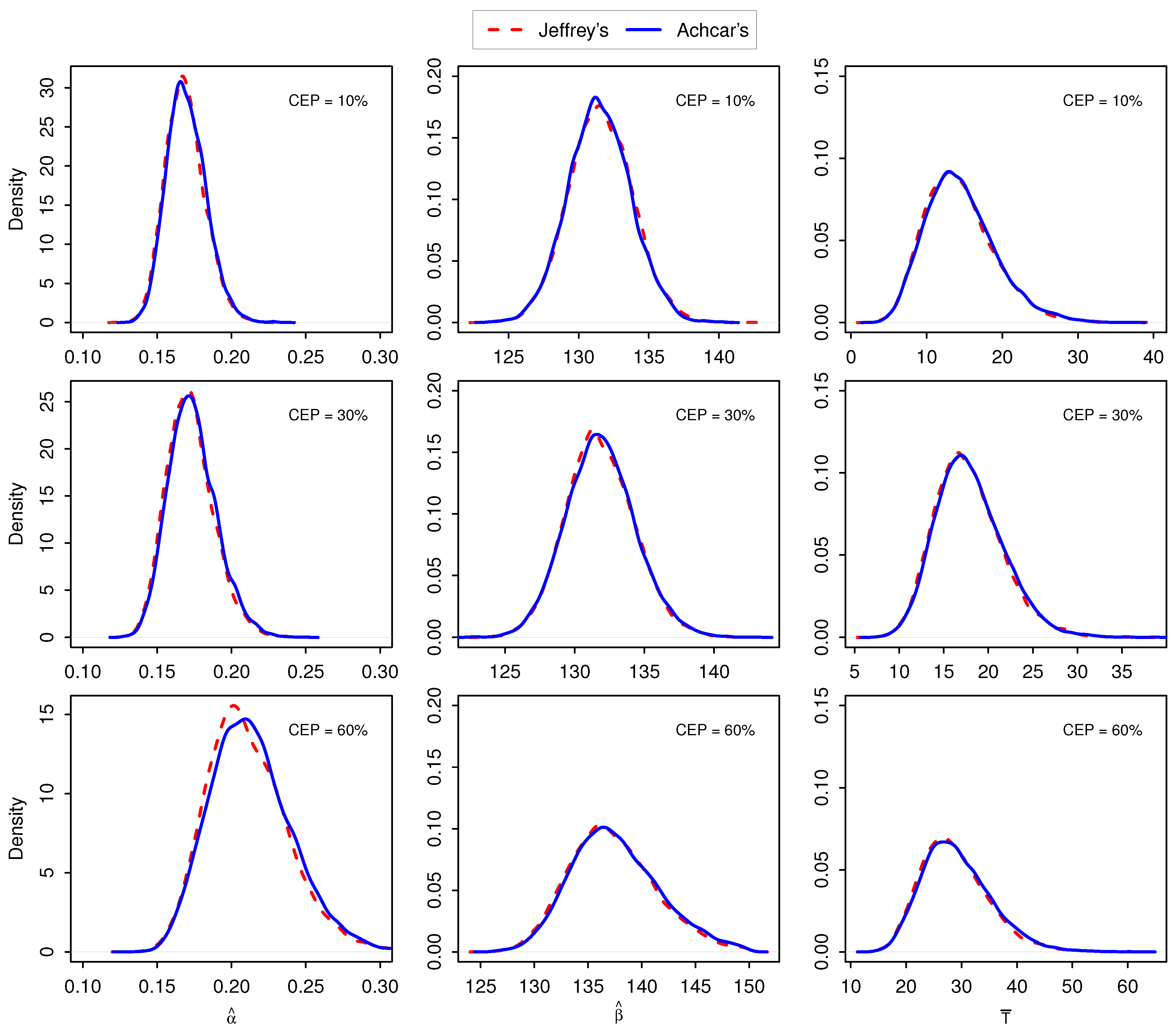
Also, Figure 1 shows the kernel density estimates of the parameters for Jeffrey’s and Achcar’s priors at 10%, 30%, and 60% censoring levels. The plots seem adequate and both methods seem to provide very similar estimates. However, as [26] indicated, the Gibbs output may not detect improper posteriors; the scale transformation we suggested should have scaled-down $\beta$ to prevent such possible divergences.

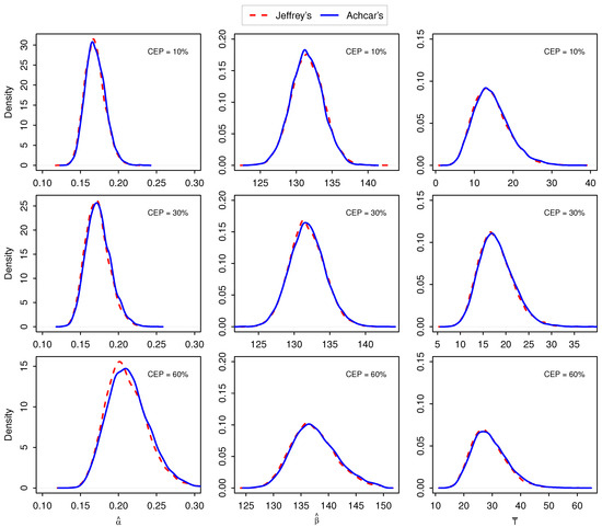
Figure 1. Kernel density estimates of Achcar’s and Jeffrey’s priors for censored fatigue life data. Top panel, middle, and bottom panels are for 10%, 30%, and 60% censoring schemes, respectively.

The resulting point estimates along with the widths of the 95% credible intervals for both the priors are reported in Table 7. Interestingly, both $\widehat{\alpha }$ and $\widehat{\beta }$ estimates for both the methods for lower to mid-censoring percentages 10%, 20%, and 30% are very close to their uncensored MLEs for complete data ($\widehat{\alpha }=0.170$ and $\widehat{\beta }=131.819$). However, when censoring percentage increases, both $\widehat{\alpha }$ and $\widehat{\beta }$ overestimate the true values. As expected, the average remaining time $\overline{T}$ is also increased with respect to the censoring percentages. It is also noted that all six $\overline{T}$ estimates overestimated the true average remaining time; the increments are proportional to the true values for increasing the censoring percentages reported in Table 6.

Table 7. Point estimates ($\widehat{\alpha }$, $\widehat{\beta }$, and $\overline{T}$) and widths of the corresponding credible intervals for different censoring percentages.

		Jeffrey’s		Achcar’s
DOC%	Param	PE	Width	PE	Width
10	$\alpha$	0.169	0.051	0.170	0.051
	$\beta$	131.582	8.926	131.501	8.796
	$\overline{T}$	14.348	17.628	14.519	18.105
20	$\alpha$	0.174	0.058	0.175	0.058
	$\beta$	131.900	9.386	131.994	9.356
	$\overline{T}$	16.318	15.297	16.421	15.277
30	$\alpha$	0.172	0.063	0.174	0.063
	$\beta$	131.830	9.601	131.883	9.876
	$\overline{T}$	17.759	14.654	17.951	14.705
40	$\alpha$	0.182	0.072	0.184	0.074
	$\beta$	132.993	10.921	133.101	11.091
	$\overline{T}$	20.405	16.228	20.691	16.533
50	$\alpha$	0.185	0.082	0.187	0.082
	$\beta$	133.276	12.267	133.469	12.271
	$\overline{T}$	22.541	17.959	22.881	18.037
60	$\alpha$	0.211	0.106	0.214	0.108
	$\beta$	137.281	15.897	137.569	16.052
	$\overline{T}$	28.768	23.985	29.227	24.213

• Example 03 (Ball Bearings’ Data): This data set was originally presented in [27] and provides the fatigue life in hours of ten ball bearings of a certain type:

152.7

172.0

172.5

173.3

193.0

204.7

216.5

234.9

262.6

422.6

Ref. [9] used the full data set and fitted BS distribution and reported that unbiased MLEs of $\alpha$ and $\beta$ are 0.314 and 211.528, respectively. Ref. [20] used these data to generate three different progressively Type-II-censored samples and estimated BS parameters. We use somewhat similar progressively Type-II-censored samples, as shown below.

• Scheme I: $n=10,m=6,R_1=4,R_2=\cdots =R_6=0;$
• Scheme II: $n=10,m=6,R_1=0,R_2=2,R_3=R_4=R_5=0,R_6=2$.

The resulting parameter estimates, along with their 95% credible intervals, are reported in Table 8. Due to censoring in this small dataset, both Bayesian priors underestimate the unbiased MLEs. However, the credible intervals adequately capture these values. Achcar’s estimates become slightly better, as they are closer to the unbiased MLEs obtained from the complete data. This example indicates that the suggested method can be used effectively even for small datasets, yielding decent results.

Table 8. Parameter estimates on Type-II progressively censored ball bearings’ data.

Parameter	$\mathit{\alpha }$		$\mathit{\beta }$		$\overline{\mathit{T}}$
	PE	95% CI	PE	95% CI	PE	95% CI
	Scheme–I
Jeffrey’s	0.182	(0.107, 0.327)	201.939	(175.660, 236.367)	57.921	(21.599, 116.568)
Achcar’s	0.199	(0.113, 0.368)	201.993	(174.342, 236.251)	60.627	(21.944, 126.152)
	Scheme–II
Jeffrey’s	0.173	(0.095, 0.337)	201.058	(178.361, 233.527)	36.467	(9.779, 94.211)
Achcar’s	0.195	(0.102, 0.400)	201.686	(177.561, 235.060)	41.159	(10.182, 109.039)

6. Conclusions

This study reveals that the suggested Gibbs sampler performs reasonably well with both Bayesian priors. Achcar’s priors appear to provide better coverage probability than Jeffrey’s prior in the considered cases of this simulation study. Additionally, Achcar’s priors tend to slightly overestimate the true parameter value, while Jeffrey’s tends to underestimate it. The amount of censoring and sample size has an impact on the performance of both methods, and therefore, one should be aware of this limitation in practice. With an increase in sample size, all methods perform better, although the amount of censoring seems to slightly affect the estimates. Care must be taken regarding the size of the $\beta$ parameter and the sample size when applying non-informative priors. The suggested scale transformation may need to be adopted to guarantee proper posteriors when using Achcar’s reference prior. Also, because the marginal posterior distributions relied on the Laplace approximation, there may be limitations on estimating the average lifetime because the BS density $T\sim BS(\widehat{\alpha },\widehat{\beta })$ is an approximation to its true underlying distribution. However, this study reveals that the Gibbs sampler is capable enough to provide accurate remaining average lifetime estimates.

The simulation results indicate that the method considered shows some improvements with regards to point estimates and coverage probabilities when compared to [15] Bayesian results. In particular, our algorithm shows no substantial effect on the coverage probability by the amount of censoring. Also, the posterior distributions discussed here have tractable closed forms that require no partial or hyper-prior information. Also, our results are consistent with regards to the bias and coverage probability for all parameter combinations we considered; this shows a clear improvement when compared to the simulation results shown in [18].

With the Gibbs sampler, there is less restriction on the type of prior distribution that can be chosen. However, caution must be exercised in programming to ensure the well-behaved nature of both prior and posterior distributions. If posterior distributions, whether conditional or otherwise, cannot be precisely determined, asymptotic distributions may be employed. The Gibbs sampler procedures offer a high degree of flexibility in implementation, allowing the adjustment of the number of iterations based on the trade-off between the speed and desired accuracy. Undoubtedly, the Gibbs sampler finds its place in developing complex models, particularly when dealing with censored data. Its computation involves a series of calculations that are easy to understand, and its implementation is relatively straightforward.

References

- Birnbaum, Z.W.; Saunders, S.C. A new family of life distributions. J. Appl. Probab. 1969, 6, 319–327. [Google Scholar] [CrossRef]
- Balakrishnan, N.; Kundu, D. Birnbaum-Saunders distribution: A review of models, analysis, and applications. Appl. Stoch. Model. Bus. Ind. 2019, 35, 4–49. [Google Scholar]
- Desmond, A.F. On the relationship between two fatigue-life models. IEEE Trans. Reliab. 1986, 35, 167–169. [Google Scholar] [CrossRef]
- Bhattacharyya, G.; Fries, A. Fatigue Failure Models—Birnbaum-Saunders vs. Inverse Gaussian. IEEE Trans. Reliab. 1982, 31, 439–441. [Google Scholar] [CrossRef]
- Owen, W.J.; Ng, H.K.T. Revisit of relationships and models for the Birnbaum-Saunders and inverse-Gaussian distributions. J. Stat. Distrib. Appl. 2015, 2, 11. [Google Scholar]
- Ng, H.K.T. Discussion of “Birnbaum-Saunders distribution: A review of models, analysis, and applications”. Appl. Stoch. Model. Bus. Ind. 2019, 35, 64–71. [Google Scholar] [CrossRef]
- Saunders, S.C. A family of random variables closed under reciprocation. J. Am. Stat. Assoc. 1974, 69, 533–539. [Google Scholar] [CrossRef]
- Birnbaum, Z.W.; Saunders, S.C. Estimation for a family of life distributions with applications to fatigue. J. Appl. Probab. 1969, 6, 328–347. [Google Scholar] [CrossRef]
- Ng, H.; Kundu, D.; Balakrishnan, N. Modified moment estimation for the two-parameter Birnbaum–Saunders distribution. Comput. Stat. Data Anal. 2003, 43, 283–298. [Google Scholar] [CrossRef]
- Balakrishnan, N.; Zhu, X. An improved method of estimation for the parameters of the Birnbaum–Saunders distribution. J. Stat. Comput. Simul. 2014, 84, 2285–2294. [Google Scholar] [CrossRef]
- Ng, H.; Kundu, D.; Balakrishnan, N. Point and interval estimation for the two-parameter Birnbaum–Saunders distribution based on Type-II censored samples. Comput. Stat. Data Anal. 2006, 50, 3222–3242. [Google Scholar] [CrossRef]
- Wang, Z.; Desmond, A.F.; Lu, X. Modified censored moment estimation for the two-parameter Birnbaum–Saunders distribution. Comput. Stat. Data Anal. 2006, 50, 1033–1051. [Google Scholar] [CrossRef]
- Jayalath, K.P. Fiducial Inference on the Right Censored Birnbaum–Saunders Data via Gibbs Sampler. Stats 2021, 4, 385–399. [Google Scholar] [CrossRef]
- Achcar, J.A. Inferences for the Birnbaum—Saunders fatigue life model using Bayesian methods. Comput. Stat. Data Anal. 1993, 15, 367–380. [Google Scholar] [CrossRef]
- Xu, A.; Tang, Y. Reference analysis for Birnbaum–Saunders distribution. Comput. Stat. Data Anal. 2010, 54, 185–192. [Google Scholar] [CrossRef]
- Xu, A.; Tang, Y. Bayesian analysis of Birnbaum–Saunders distribution with partial information. Comput. Stat. Data Anal. 2011, 55, 2324–2333. [Google Scholar] [CrossRef]
- Wang, M.; Sun, X.; Park, C. Bayesian analysis of Birnbaum–Saunders distribution via the generalized ratio-of-uniforms method. Comput. Stat. 2016, 31, 207–225. [Google Scholar] [CrossRef]
- Sha, N.; Ng, T.L. Bayesian inference for Birnbaum–Saunders distribution and its generalization. J. Stat. Comput. Simul. 2017, 87, 2411–2429. [Google Scholar] [CrossRef]
- Balakrishnan, N.; Cramer, E. The art of progressive censoring. In Statistics for Industry and Technology; Springer: Berlin/Heidelberg, Germany, 2014. [Google Scholar]
- Pradhan, B.; Kundu, D. Inference and optimal censoring schemes for progressively censored Birnbaum–Saunders distribution. J. Stat. Plan. Inference 2013, 143, 1098–1108. [Google Scholar] [CrossRef]
- Delignette-Muller, M.; Dutang, C. An R Package for Fitting Distributions. J. Stat. Softw. 2015, 61, 1–34. [Google Scholar]
- R Core Team. R: A Language and Environment for Statistical Computing; R Foundation for Statistical Computing: Vienna, Austria, 2019. [Google Scholar]
- Brooks, S.P.; Gelman, A. General methods for monitoring convergence of iterative simulations. J. Comput. Graph. Stat. 1998, 7, 434–455. [Google Scholar]
- Gelman, A.; Carlin, J.B.; Stern, H.S.; Dunson, D.B.; Vehtari, A.; Rubin, D.B. Bayesian Data Analysis; Chapman and Hall/CRC: Boca Raton, FL, USA, 2013. [Google Scholar]
- Achcar, J.A.; Moala, F.A. Use of MCMC methods to obtain Bayesian inferences for the Birnbaum-Saunders distribution in the presence of censored data and covariates. Adv. Appl. Stat. 2010, 17, 1–27. [Google Scholar]
- Hobert, J.P.; Casella, G. The effect of improper priors on Gibbs sampling in hierarchical linear mixed models. J. Am. Stat. Assoc. 1996, 91, 1461–1473. [Google Scholar]
- McCool, J. Inferential Techniques for Weibull Populations. Aerospace Research Laboratories Report; Technical Report, ARL TR 74-0180; Wright-Patterson AFB: Fairborn, OH, USA, 1974. [Google Scholar]
Disclaimer/Publisher’s Note: The statements, opinions and data contained in all publications are solely those of the individual author(s) and contributor(s) and not of MDPI and/or the editor(s). MDPI and/or the editor(s) disclaim responsibility for any injury to people or property resulting from any ideas, methods, instructions or products referred to in the content. |
© 2024 by the author. Licensee MDPI, Basel, Switzerland. This article is an open access article distributed under the terms and conditions of the Creative Commons Attribution (CC BY) license (https://creativecommons.org/licenses/by/4.0/).