Abstract
Landslide displacement prediction is of great significance for the prevention and early warning of slope hazards. In order to enhance the extraction of landslide historical monitoring signals, a landslide displacement prediction method is proposed based on the decomposition of monitoring data before prediction. Firstly, based on the idea of temporal addition, the sparrow search algorithm (SSA) coupled with the variational modal decomposition (VMD) algorithm is used to decompose the total landslide displacement into trend item, periodic item and random item; then, the displacement values of the subitems are fitted by using the long and short-term memory (LSTM) neural network, and the predicted cumulative landslide displacement is obtained by adding up the predicted values of the three subsequences. Finally, the historical measured data of the Shuping landslide is taken as an example. Considering the effects of seasonal rainfall and reservoir water level rise and fall, the displacement of this landslide is predicted, and the prediction results of other traditional models are compared. The results show that the landslide displacement prediction model of SSA-VMD coupled with LSTM can predict landslide displacement more accurately and capture the characteristics of historical signals, which can be used as a reference for landslide displacement prediction.
Keywords:
landslide displacement prediction; time series; sparrow search algorithm; variational modal decomposition; long and short-term memory neural network; bank landslide MSC:
68T07
1. Introduction
Landslide disasters occur all over the world, seriously threatening people’s lives and economic development [1,2,3]. For example, the landslide disaster that occurred in Wuxi County, Chongqing, China, in June 2022 resulted in two deaths, three missing persons, and enormous economic loss. Landslide displacement prediction, as an important geological disaster prevention measure, is an indispensable part of landslide early warning work. The establishment of a safe and reliable landslide displacement prediction model is of great significance for disaster prevention. While the Three Gorges reservoir area is a landslide disaster-prone area in China, it is necessary to carry out monitoring and prediction of landslide disasters [4,5,6].
Landslide displacement prediction models have evolved from Saito’s creep theory [7] in the 1960s to empirical prediction models, mathematical–statistical models, nonlinear models and comprehensive prediction models. The empirical prediction model is a prediction method based on the observed sharp increase in deformation before landslide destabilization [8,9]. The time of landslide destabilization is predicted by analysis and derivation on a physical model [10]. This prediction method is based on specific experimental observations. It is limited in applicability and scalability. Mathematical–statistical models are prediction tools built on the basic theory of mathematics and statistical methods; the common ones are the Verhulst model [11,12] and the gray theory model [13,14]. However, such models cannot be linked to the intrinsic mechanism of landslide deformation, and the prediction accuracy needs to be improved. In addition, it is gradually recognized that landslide deformation is a complex nonlinear process with sudden and gradual changes [15]. Therefore, the nonlinear theory is gradually applied in the destabilization prediction of landslide deformation [16]. However, since landslide deformation is jointly influenced by a variety of factors, it is difficult for the statistical model to reflect the volatility of displacement with these influencing factors. It cannot be well considered in connection with the time variable in the process of landslide deformation, which has some limitations.
In order to further improve the performance of the prediction model, scholars coupled multiple models together to establish a more comprehensive landslide displacement-integrated prediction model. According to the idea of time series addition, cumulative landslide displacement can be decomposed into subsequences reflecting different characteristics, which usually include trend displacement, periodic displacement and random displacement [17,18]. The commonly used decomposition methods include wavelet analysis (WA) [19], empirical modal decomposition (EMD) [20,21], ensemble empirical mode decomposition (EEMD) [22,23] and variational modal decomposition (VMD) [24,25]. The VMD shows better decomposition in landslide cumulative displacement decomposition. In this paper, the variational modal decomposition algorithm, which has better decomposition accuracy for complex data, is used to decompose the landslide displacement time series signal. Among them, the selection of model parameters has a great influence on the decomposition accuracy. At present, the selection of machine learning model parameters is mainly iteratively optimized by particle swarm algorithm (PSO), genetic algorithm (GA) [26,27], whale optimization algorithm (WOA) [28] and so on. The sparrow search algorithm (SSA) has the advantages of fast convergence, high accuracy and robustness compared with other optimization algorithms [29]. Therefore, this paper adopts the sparrow search algorithm to solve the parameters of the variational modal decomposition. For the landslide displacement prediction model, traditional machine learning methods such as support vector machine (SVM) [30,31] and BP neural network [32,33] have been widely used in landslide displacement prediction, but these static models failed to consider the time factor, and the displacement value is regarded as an isolated point for regression prediction. Landslide deformation is a time-varying physical phenomenon, and time-series prediction models, such as the long and short-term memory (LSTM) neural network, have natural advantages for time-varying problems [34,35]. Therefore, this paper adopts the LSTM model to predict the decomposed landslide displacement subsequences.
In summary, this paper takes the Shuping landslide in the Three Gorges Reservoir Area as the research object and proposes a landslide displacement prediction model combining the sparrow search algorithm, variational modal decomposition algorithm and the long and short-term memory neural network. Firstly, the landslide monitoring displacement sequence is decomposed by the SSA-VMD model to extract the trend displacement, periodic displacement and random displacement. Secondly, we analyze the influencing factors of the periodic item of landslide displacement and realize the prediction of the characteristic subsequences of landslide displacement through the LSTM model so as to superpose the predicted value of landslide cumulative displacement in order to provide a reference for slope engineering research.
2. Materials and Methods
2.1. Temporal Addition Model
The landslide cumulative displacement profile can be decomposed into different characteristic subsequences using the temporal addition model.
where is the cumulative displacement value; is a trend displacement, mainly reflecting the deformation pattern of the slope itself, generally showing a monotonically increasing change; is a periodic displacement, reflecting the influence of the slope by external factors, such as reservoir level fluctuations and rainfall, which shows a cyclic-like curve; is random displacement, reflecting the effects of sudden factors, such as wind loads and artificial loads, which is presented as a high-frequency stochasticity curve.
2.2. VMD
Variational mode decomposition (VMD) is able to decompose the raw data signal into multiple intrinsic modal function (IMF) components with their own characteristics. The VMD model is based on the variational method, which decomposes the signal by constructing a variational problem to find an optimal solution [36]. The goal of the algorithm is to adaptively separate these modes and estimate the center frequency and bandwidth of each mode. To achieve this goal, the algorithm uses a completely non-recursive approach to modal decomposition, avoiding the problem of modal aliasing that exists in traditional signal decomposition algorithms. The VMD model ultimately has to achieve all components adding up to the original sign.
Each IMF component can be expressed as a modal function:
where is the amplitude, and ; is the instantaneous phase angle, and its derivation with respect to time gives the instantaneous power:
The modal functions are Hilbert transformed:
The modal functions are tuned to their respective fundamental frequency bands:
The constrained variational problem in VMD can be written as:
where is the original signal; is the predicted center frequency of each component; is the unit pulse function.
Introducing quadratic penalty factors and Lagrange multipliers and converting constrained variational models to augmented Lagrange expressions for unconstrained models:
The variational problem of the above equation is solved using the multiplier alternating direction method, which decomposes the input signal into multiple components by updating , and to find the Lagrange saddle points of this equation.
2.3. SSA-VMD
The VMD algorithm has two preset parameters: the modal decomposition number and the penalty factor . When is too small, signals with similar center frequencies will be decomposed into the same IMF components, resulting in a modal mixing problem. On the contrary, when is too large, some useless false signals will be generated. The parameter determines the bandwidth of the IMF component; if it is too small, it may lead to signal loss. If it is too large, it may lead to signal mixing. In order to solve this problem effectively for the landslide cumulative displacement signals, we proposed an optimized signal decomposition method using the SSA algorithm to determine the VMD initial parameters.
Sparrow search algorithm (SSA) is an optimization algorithm derived from biological behaviors based on nature that seeks optimal solutions by drawing on the foraging and collaborative behaviors of sparrows. Individual sparrows play different roles in the foraging process, with the discoverer providing the direction and location of food for the entire population and the joiner obtaining food through the discoverer. When there is a predator in the vicinity, the detector gives an alert so that the population can avoid the danger [37]. The rules for updating the location of each role are as follows:
The discoverer’s location update equation is:
where is the location of an individual; is the maximum number of iterations; and are the warning and safety values, respectively.
The joiner’s location update equation is:
where is optimal positions occupied by producers; is the worst position in the whole world; is the size of the population.
The defender’s location update equation is:
where is the current global optimal position; is the step control parameter; , and are the fitness values, worst and optimal fitness values.
When using the SSA algorithm to optimize the VMD parameters, it is crucial to choose an appropriate fitness function. This function will affect the convergence speed of the SSA algorithm and will also determine whether the optimal solution can be searched in the end. The landslide cumulative displacement signal is a time series signal. Envelope entropy is a reliable fitness function, which is confirmed in different time series signal decomposition studies. Therefore, the envelope entropy is used in the SSA-VMD model. The envelope signal obtained from signal decomposition can be transformed into a sequence of probability distributions, and this sequence is used to calculate the envelope entropy, which, in turn, reflects the sparse characteristics of the original time-series signal. The envelope entropy of component is calculated as follows:
where is the envelope signal after the Hilbert transform and is its standardized form.
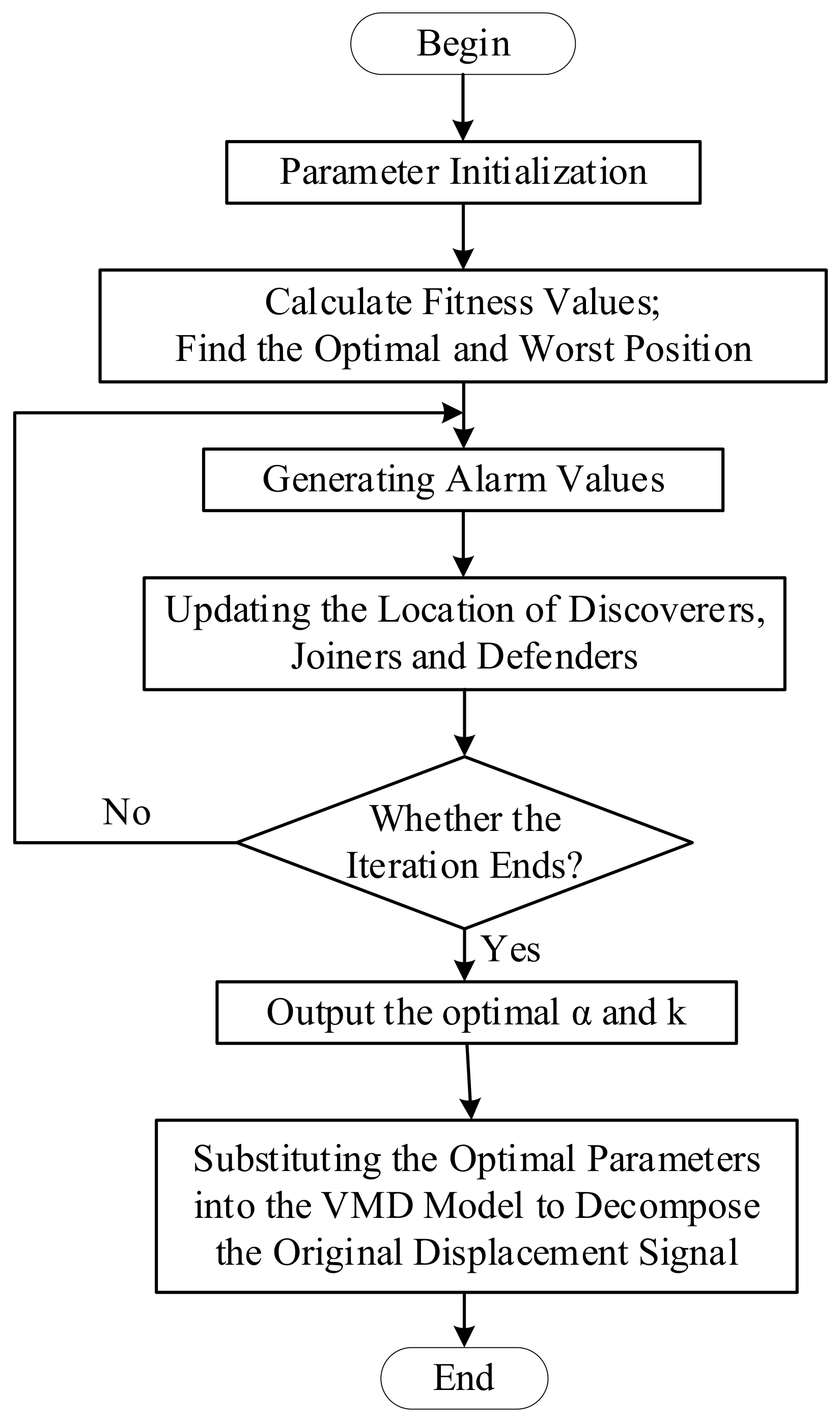
When the envelope entropy is used for optimization, the minimum value of the envelope entropy is used as the fitting function, which can obtain more displacement components that are in line with the information of the actual landslide influence factors and is conducive to improving the accuracy of the cumulative displacement decomposition. The minimum value of envelope entropy is calculated according to a series of IMF components under the combination of parameters and . The minimum entropy value corresponds to the optimal and . The signal decomposition process based on the SSA algorithm with the VMD model is shown in Figure 1.
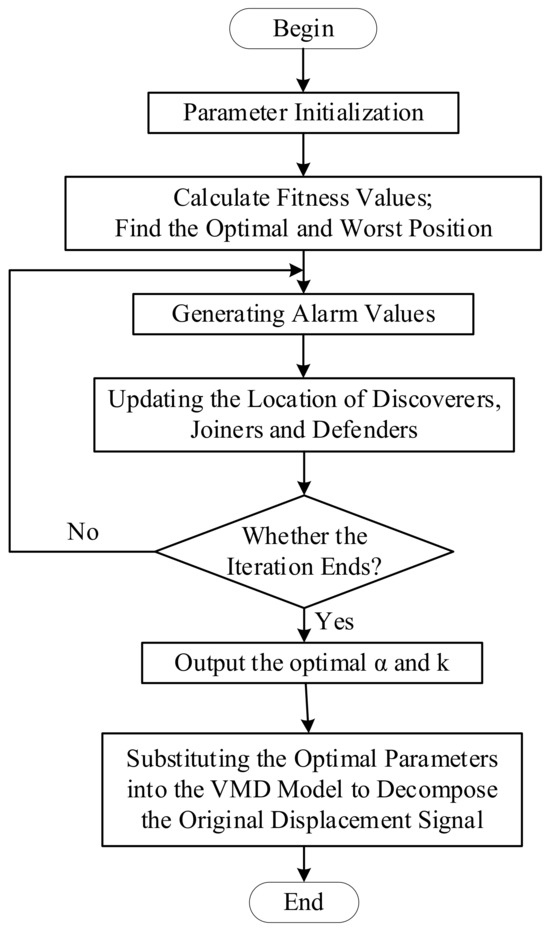
Figure 1.
Flow chart of variational modal decomposition (VMD) optimized by sparrow search algorithm (SSA).
2.4. LSTM
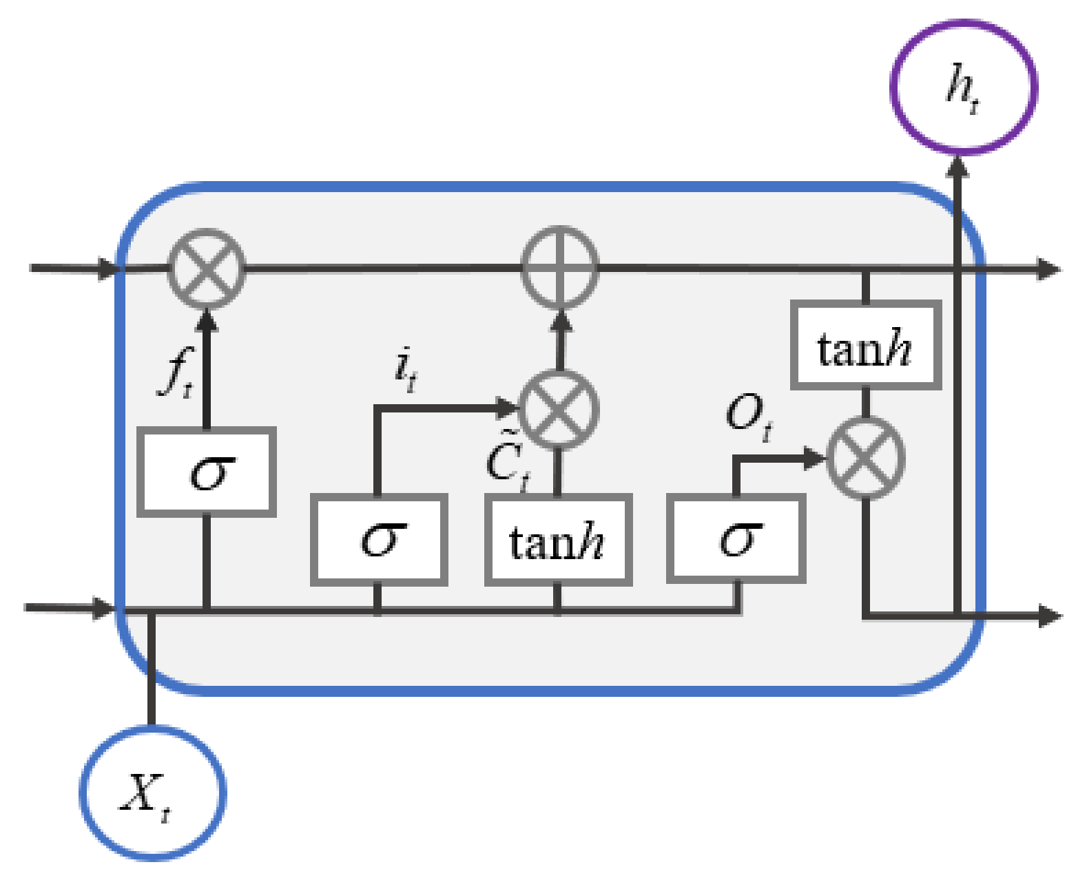
Long and short-term memory (LSTM) is used to establish long-term dependency relationships, which adds input gates, output gates and forgetting gates on the basis of a recurrent neural network (RNN) to solve the problem of gradient disappearance and gradient explosion of RNN in long sequences. The LSTM model possesses a good memory ability, which is able to effectively transfer the temporal information backward in the prediction of landslide displacements and improves the prediction accuracy. The structure of the LSTM unit is shown in Figure 2.
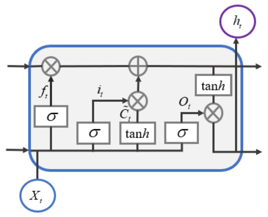
Figure 2.
Long and short-term memory (LSTM) unit.
The Oblivion Gate is used to retain important information from the previous moment:
where and are the weights and bias of the forgetting gate activation function.
The input gate determines the reserved information in the input signal at moment and in the output signal at moment :
where and are the weights and bias of the input gate activation function; and are the weights and bias of the input gate activation function; is the newly obtained cell state information.
The output gate determines the next layer of hidden information:
where and are the weights and bias of the output gate activation function.
2.5. Evaluation Indicators
Landslide displacement prediction is a typical regression problem. To evaluate the prediction ability of the model, root mean squared error (RMSE), mean absolute error (MAE) and goodness of fit (R2) are selected as the model performance evaluation indicators. RMSE and MAE are error indicators; compared with other indicators, these two can directly reflect the degree of deviation between the predicted value and the real value—a smaller degree of deviation indicates that the model’s prediction effect is better. R2 reflects the degree of fit between the predicted curve and the real curve; a value close to 1 indicates the model’s fitting effect is good.
where is the sample size; , and represent the true, predicted and average of the true values of the data.
3. Results
3.1. A Real Case
In this paper, the Shuping landslide in the Three Gorges reservoir area was selected for example verification. Shuping landslide is located on the south bank of the Yangtze River in Shuping village, Zigui county, Hubei province, 47 km away from the Three Gorges Dam. The landslide has a high topography in the southwest and a low topography in the northeast, presenting a chair-like shape. The landslide belongs to the ancient avalanche accumulation body, north–south spreading, by the Triassic Badong group mudstone, siltstone sandstone and marl composed of the inverse slope to the section, a stratigraphic production tendency of 120~173° and a dip angle of 9~38°. The longitudinal length of the landslide is about 800 m from north to south, and the width is about 700 m from east to west, with a thickness of about 30~70 m and an average thickness of about 50 m.
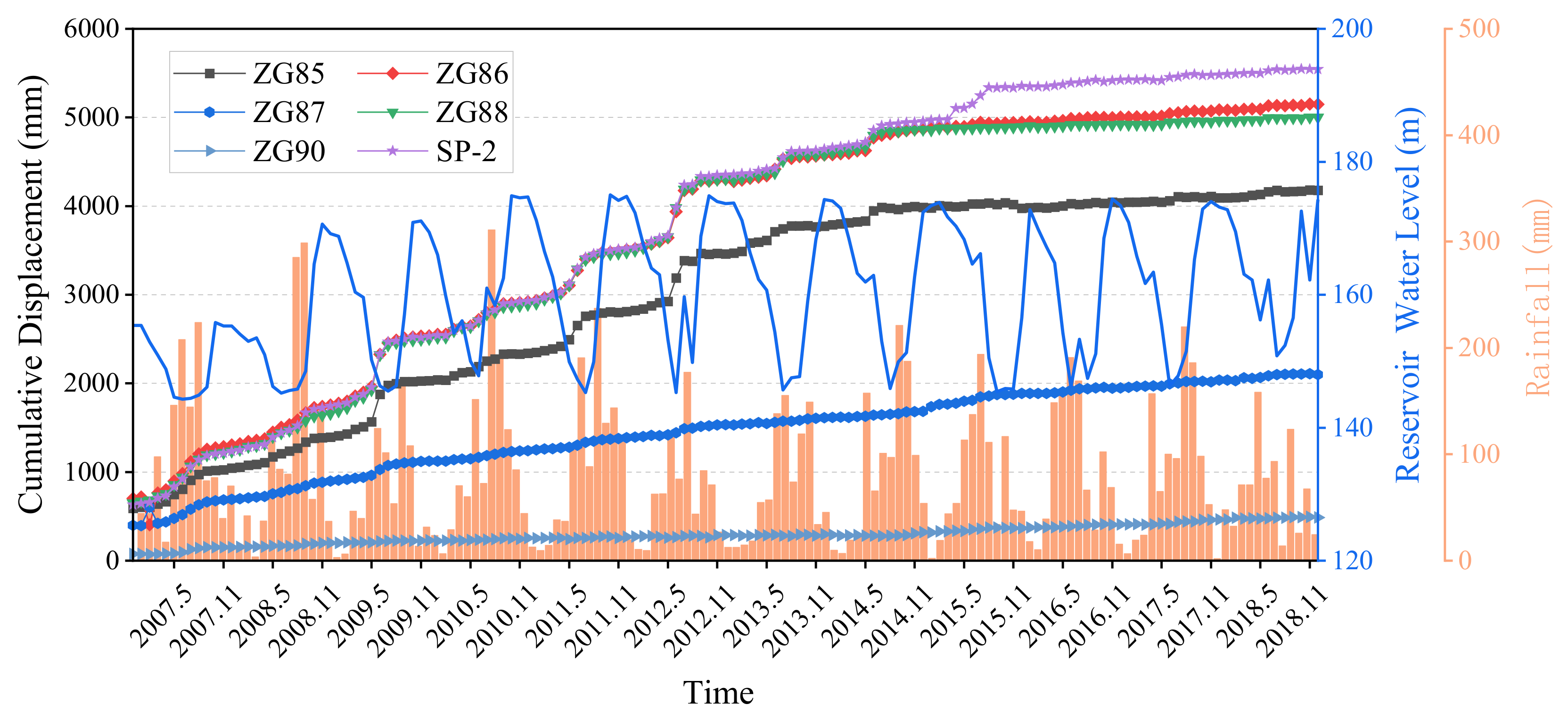
The six GPS monitoring points set up at the initial stage of monitoring are overall presented as two vertical and three horizontal arrangements, which are basically able to monitor the whole slope. According to the multi-year deformation characteristics, the Shuping landslide is divided into the main slide area and the impact area. In this paper, the monitoring data from December 2006 to December 2018 of monitoring point ZG85, which has more intense deformation within the main slide area, were selected for analysis and prediction. Among them, the monitoring values of the cumulative displacement, monthly rainfall and the average elevation of the reservoir level are shown in Figure 3.
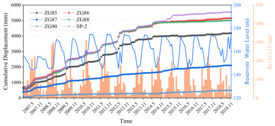
Figure 3.
Monitoring data of the Shuping landslide.
According to Figure 3, the landslide displacement, along with rainfall and reservoir water level rise and fall, presents a “step-like” characteristic, and the displacement monitoring curve will appear as a more obvious deformation growth every year. May to August every year is the reservoir flood season, during which rainfall increases while the reservoir water level drops to a low point, which has a significant impact on the stability of the slope. From September to April, the precipitation in the area decreases, and the deformation of the landslide tends to level off. Under the cyclic effect of precipitation and reservoir level, the landslide displacement showed a significant increase with some lag.
3.2. Landslide Displacement Sequence Decomposition Results
3.2.1. VMD Parameter Optimization
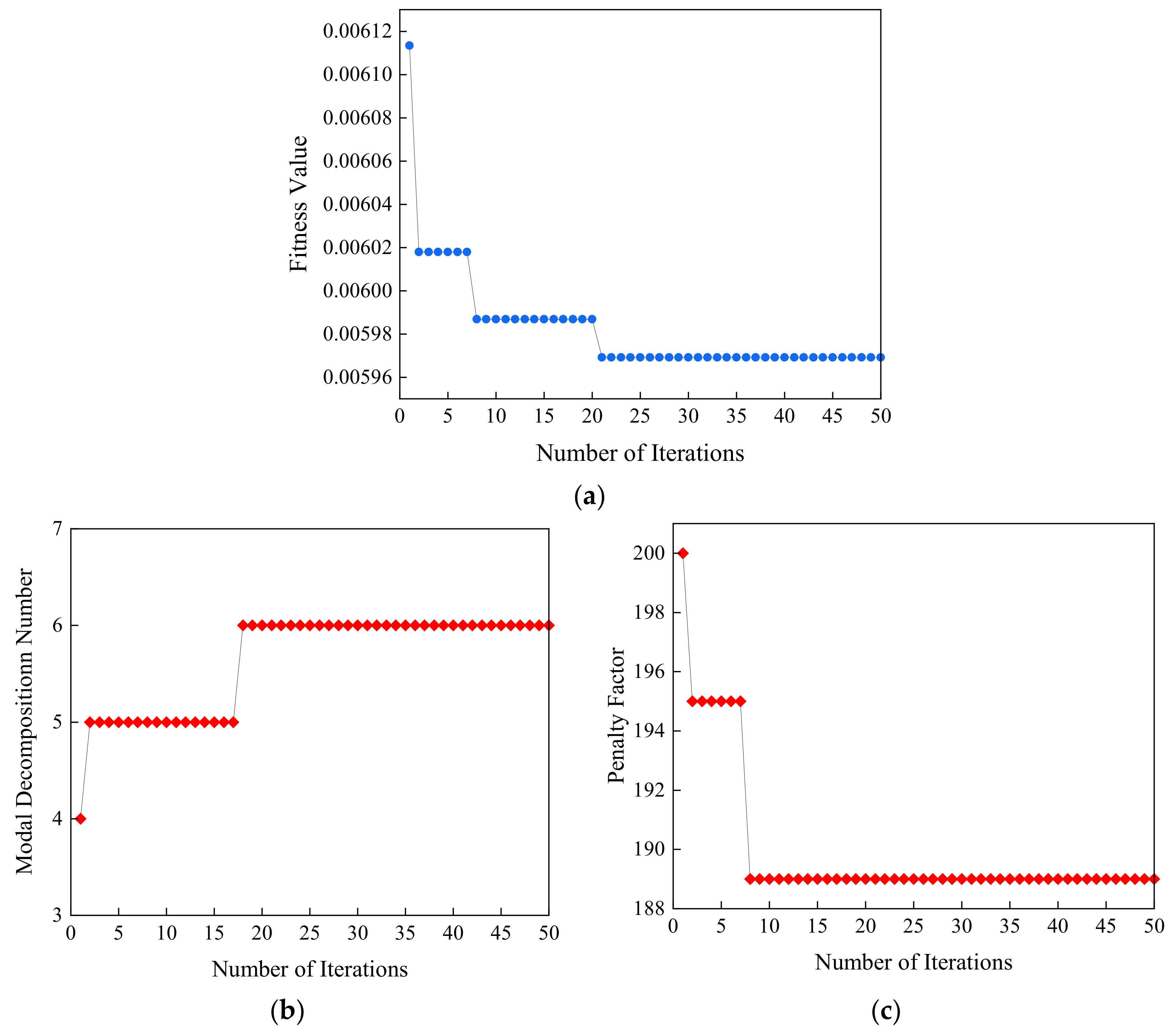
In SSA, the population size was set to 100, the maximum number of iterations was set to 50, the optimization range of the penalty factor was set to [6, 1000], and the optimization range of the modal number was set to [3, 10]. During the iteration process, the fitness value dropped rapidly to the optimal value of 0.00596, and the convergence effect was obvious, as shown in Figure 4. The optimal parameters of modal number and penalty factor are: , . The iterative process of the modal decomposition number and the penalty factor is shown in Figure 4.
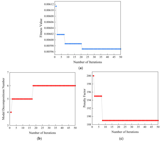
Figure 4.
Iteration curve. (a) Iteration curve of fitness. (b) Iteration curve of modal decomposition number. (c) Iteration curve of penalty factor.
3.2.2. Cumulative Displacement Decomposition Results
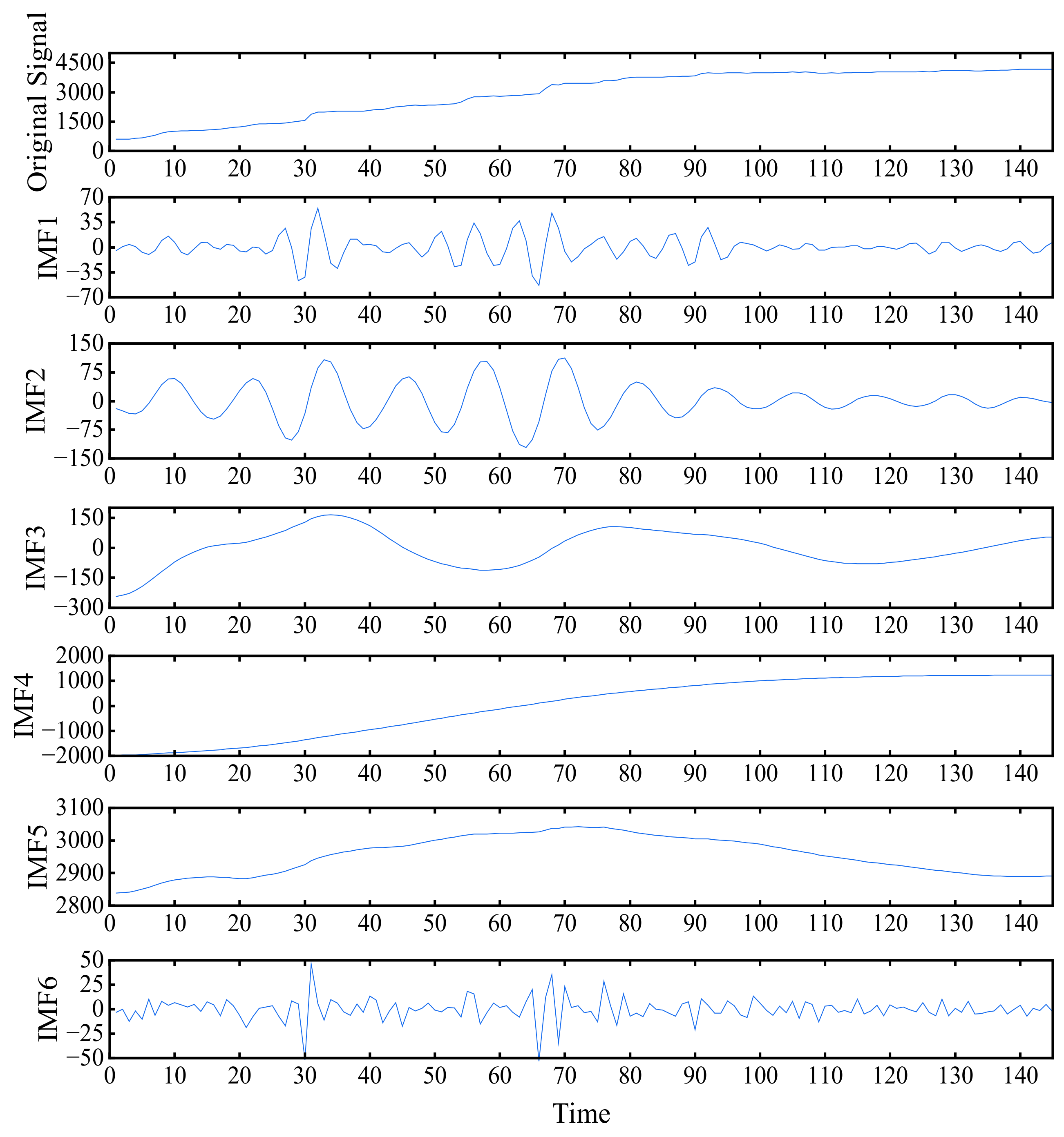
The influencing factors of landslide deformation are complicated, the monitoring data content is limited, and the stability and accuracy of the prediction results cannot be guaranteed by directly using a single variable for prediction. Therefore, the displacement signal of monitoring point ZG85 was first decomposed and then predicted to increase the details of the signal and improve the accuracy of prediction. The parameters obtained from the optimization of the SSA algorithm are used to replace the initial parameters of the VMD algorithm to ensure the decomposition effect of the landslide displacement sequence, and the decomposition results are shown in Figure 5.
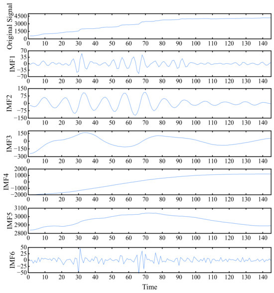
Figure 5.
Results of landslide cumulative displacement decomposition.
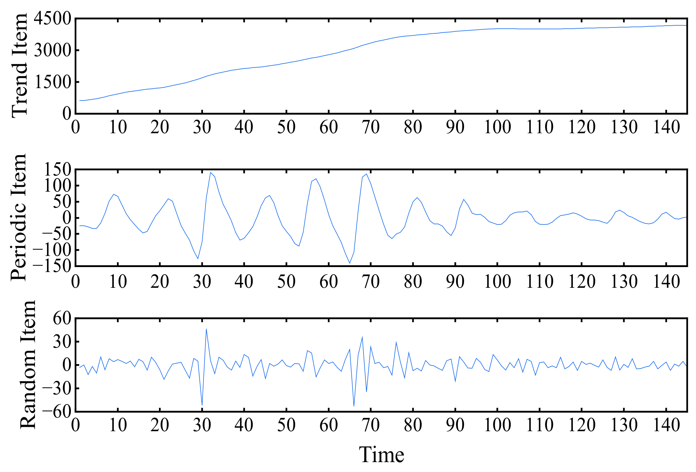
The VMD model decomposes the cumulative displacement signal of monitoring point ZG85 into six components, IMF1~IMF6, which have obvious characteristic terms. Among them, IMF1 and IMF2 show the characteristics of periodic changes. The periodic characteristics of the first 100 data points (December 2006~February 2014) are more significant, and the amplitude of fluctuations is higher. This is because the cumulative displacement of the Shuping landslide has continued to increase, and damage has been produced in some areas. The relevant departments treated the Shuping landslide and completed their operations in March 2015. IMF1 and IMF2 are superimposed to construct the periodic item of the displacement sequence. The IMF6 component shows high-frequency characteristics and no obvious pattern, which is in line with the characteristics of the random item of landslide displacement. IMF4 shows a monotonically increasing trend, which is in line with the characteristics of the trend item. IMF4, IMF3 and IMF5 are superimposed and combined to construct the trend item of the displacement sequence. The trend item, periodic item and random item obtained after the reorganization of each component are shown in Figure 6.
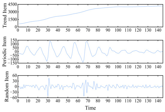
Figure 6.
Reorganized feature items.
3.3. Landslide Displacement Prediction Results
In order to consider the influence of different factors on the landslide displacement, the historical displacement monitoring sequence of Shuping landslide ZG85 was decomposed and reconstructed into three subsequences, namely, trend item, periodic item and random item, by means of the variational modal decomposition algorithm. Then, the three subsequences were predicted using the LSTM model, and the predicted displacement values of each subsequence were superimposed to obtain the predicted cumulative displacement of the landslide.
Since the LSTM time-series prediction model predicts the landslide displacement value of the next point based on the previous sequence points, the time step reflects the number of input previous sample points needed to predict the next point. Setting the input time step to 12 can reflect the displacement changes in the previous year of the predicted point and provide more comprehensive information.
The samples were divided into training set and test set according to 7:3. The training set data were from December 2007 to August 2015, with a total of 93 sets of data; the test set data were from September 2015 to December 2018, with a total of 40 sets of data. Then, the displacement signal was adjusted to between [−1, 1] by using the normalization method, and the calculation formula is as follows:
where is the value after the normalization operation; and are the minimum and maximum values in the original data series.
3.3.1. Result of Trend Item
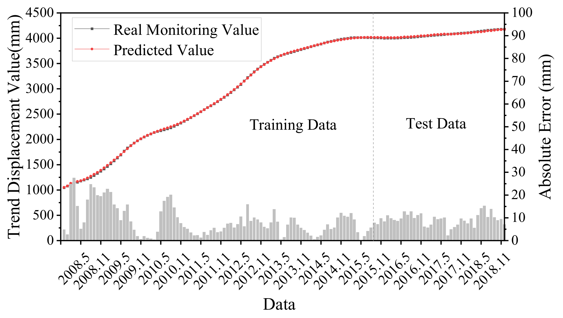
Influenced by the characteristics of the slope body and constraints, the trend item shows monotonically increasing changes over time, mainly reflecting that the landslide is influenced by its own factors. The univariate LSTM model is used to predict the future displacement change on the basis of the historical trend displacement information. The optimization algorithm chose the Adam algorithm. After several experiments and simulations, the initial learning rate was set to 0.005, the number of neurons in the implicit layer was set to 128. The prediction results and errors are shown in Figure 7, in which the R2 was 0.9642, the MAE was 9.27 mm, the RMSE was 9.64 mm and the overall change trends of the predicted and real values were more consistent.
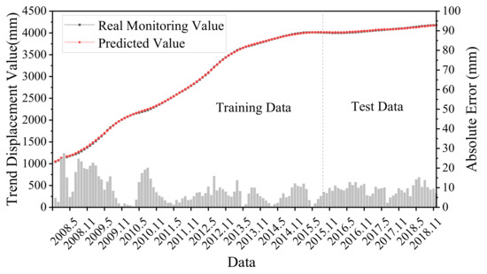
Figure 7.
Predicted and monitored trend displacement components.
3.3.2. Result of Periodic Item
- (1)
- Selection of Impact Factors
For the reservoir bank landslide, the rise and fall of the reservoir level and rainfall were the main factors leading to the step-like deformation of this landslide. The change in reservoir water level was the main inducer of landslide deformation. During the rise of the reservoir level, the river water penetrated slowly into the interior of the slope body, forming a penetration pressure pointing towards the interior of the slope body, which was conducive to the stability of the slope body. During the period of falling reservoir level, the cumulative displacement curve shows a step-like jump. This is because when the water level drops, the groundwater gradually seeps out of the slope, but the seepage of water takes a certain amount of time, resulting in the change of groundwater level slower than the reservoir level, forming the infiltration pressure pointing to the outside of the slope, the downward sliding force becomes larger and there is a certain hysteresis in response to landslide deformation. Rainfall on the landslide deformation has a promotional effect. Rainfall from the nodal fissure infiltration to the interior of the slope body, so that the water table rises, seepage field, stress field changes, the self-weight of the slope body increases, while soaked in rainwater in the rock and soil body softening, physical and mechanical strength is reduced, affecting the stability of the slope body [38,39]. In addition, at different stages of evolution, landslides produce different deformation responses to the same external triggering factors. At the early stage of landslide deformation, the triggering factors do not have a serious impact on landslide safety. When the landslide deformation accelerates and enters the later stage, some slight disturbances will accelerate the landslide deformation [40].
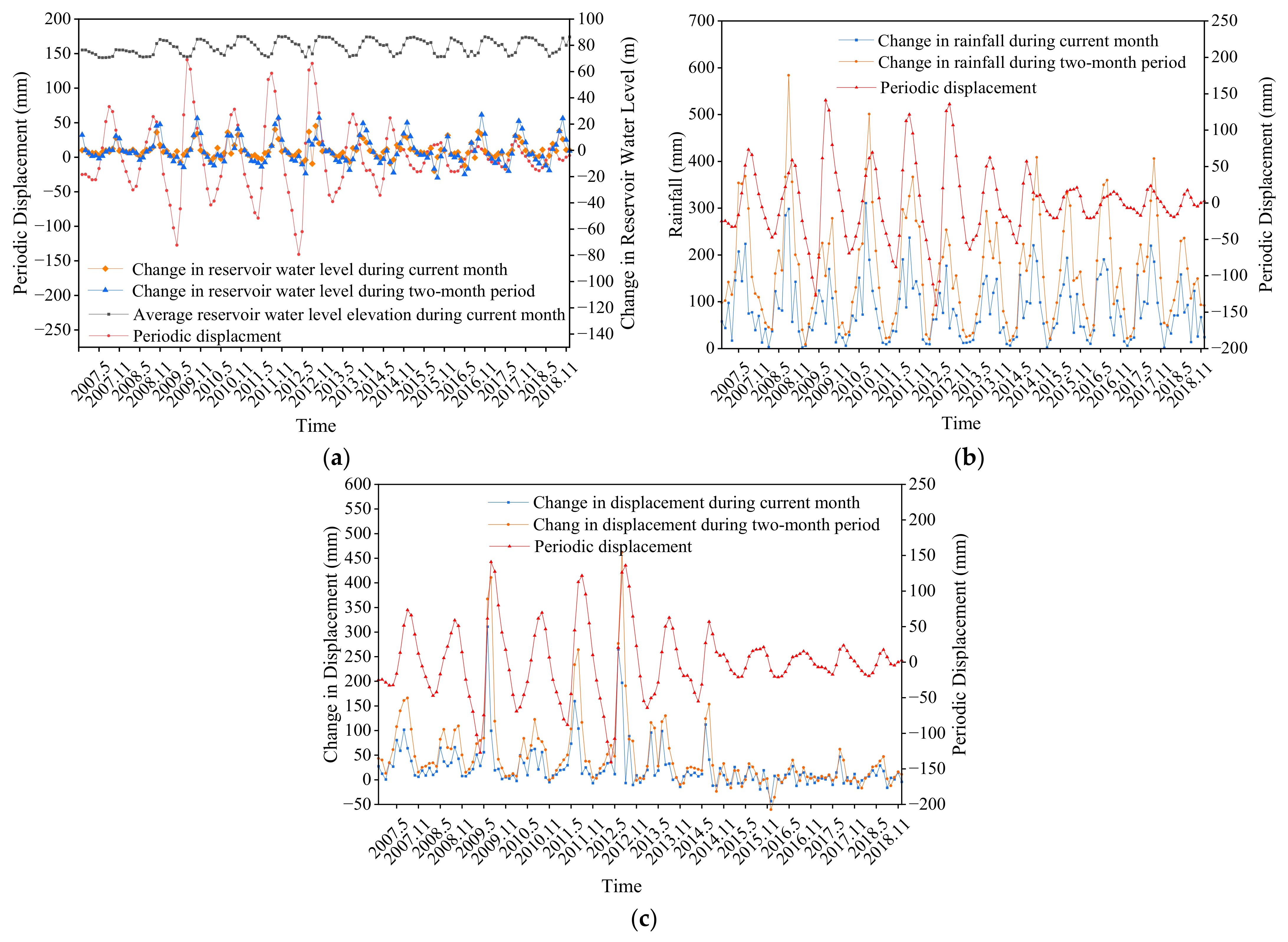
Therefore, the reservoir water level, rainfall and displacement response are taken as the influencing factors for the cyclic change of landslide displacement. The change in reservoir water level during the current month, the change in reservoir water level during the two-month period, the average reservoir water level elevation during the current month, the change in rainfall during the current month, the change in rainfall during the two-month period, the change in displacement during the current month and the change in displacement during the two-month period were selected as the input features of the model. Figure 8 demonstrates the relationship between the landslide displacement period term and each influencing factor. It can be noticed that the selected impact factors and the periodical terms all showed similar cyclical variations.
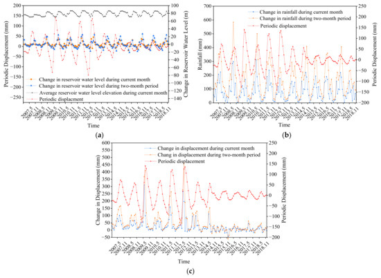
Figure 8.
Relationship between the displacement of the periodic term and the impact factor. (a) Description of reservoir level. (b) Description of rainfall. (c) Description of displacement response.
To further determine the correlation between the input features and the periodic displacement, the gray correlation analysis method was used to calculate the correlation between each influence factor and the landslide periodic displacement. According to the gray correlation theory, when setting the discrimination coefficient to 0.5, if the correlation is more than 0.6, it means that the influence factors have a close relationship with the periodic term. The analysis results are shown in Table 1. The correlation of all seven factors was greater than 0.6. Therefore, these seven influencing factors were used as input features of the model.

Table 1.
Gray correlation results.
- (2)
- Result of Periodic Displacement
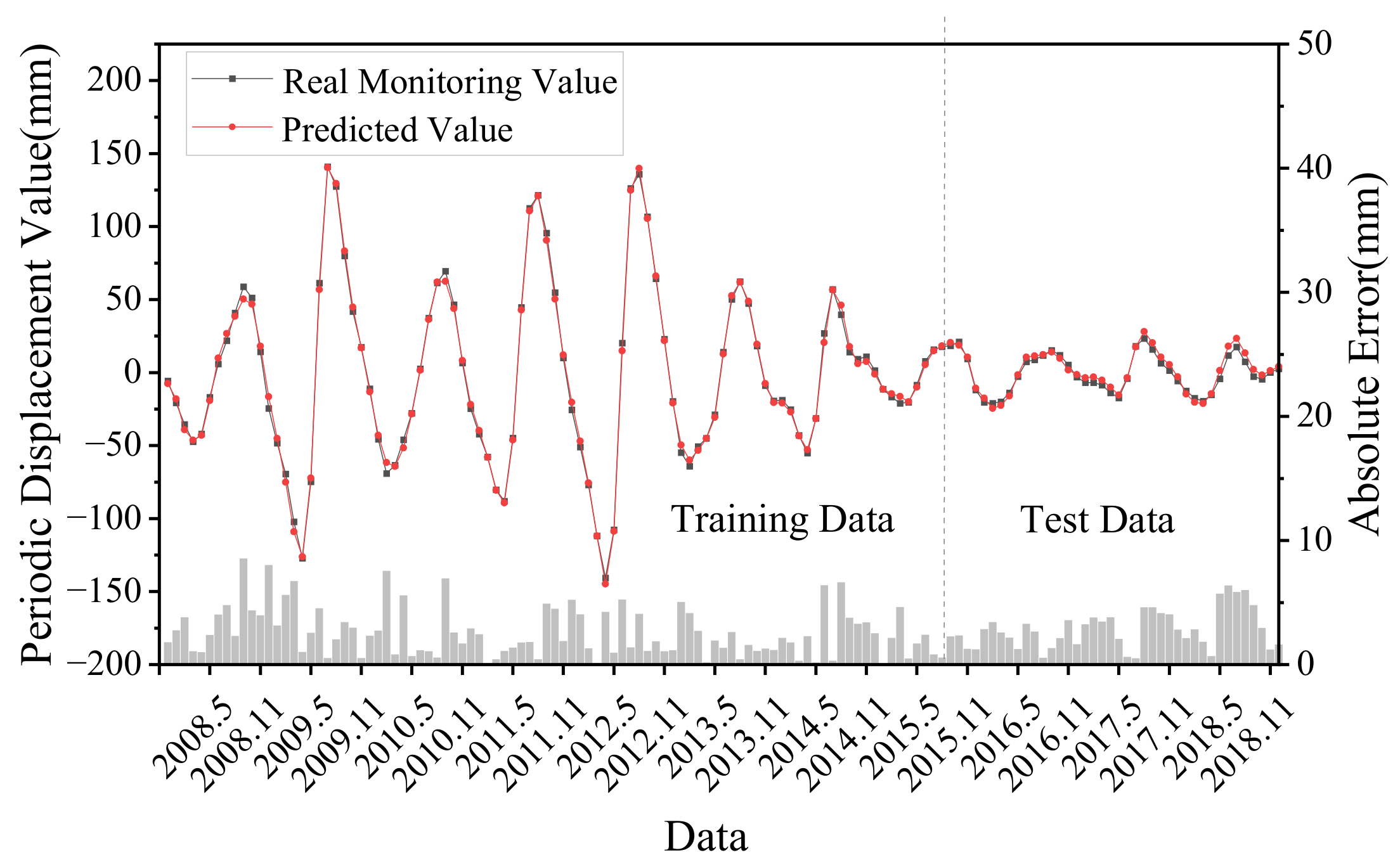
The prediction results and errors of the multivariate LSTM model applied to the displacement of periodic terms are shown in Figure 9. The input feature dimension of the model was 8, and the output feature dimension was 1. The optimization algorithm was chosen as the Adam algorithm. After several experiments and simulations, the initial learning rate was taken as 0.005 and the number of neurons in the implicit layer was set to 256. For evaluation indicators, the R2 of the periodic item was 0.947, the MAE was 2.82 mm and the RMSE was 3.22 mm. The overall prediction error was small, which can better fit the fluctuation pattern of displacement data and capture the intrinsic connection between the data.
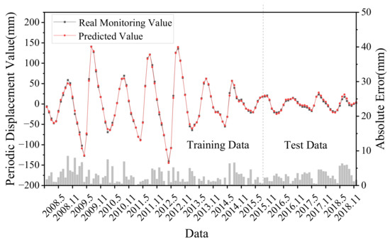
Figure 9.
Predicted and monitored periodic displacement components.
3.3.3. Result of Random Item
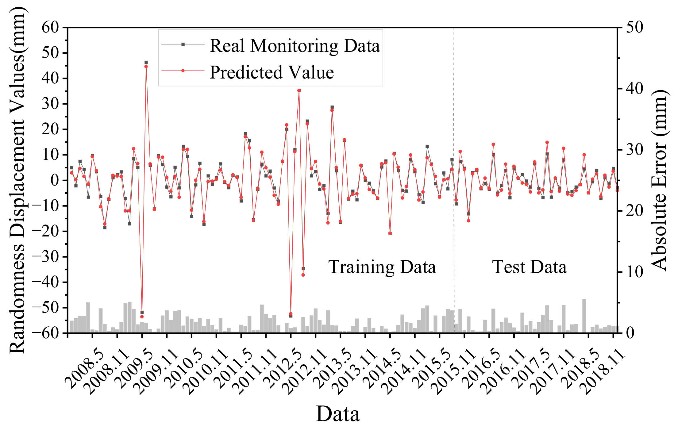
Due to the limitations of the current monitoring technology means and related research, there is a lack of data on the influencing factors of the random term of landslide displacement, so the stochasticity is only considered the influence of its own sequence. The univariate LSTM model was used to predict the displacement of the random item, with the same parameter settings as that of the trend term prediction model. The prediction results are shown in Figure 10. The evaluation index R2 was 0.893, MAE was 1.63 mm and RMSE was 2.12 mm. The goodness of fit of the random term was lower compared with the trend term and the periodic term due to the uncertainty of the influencing factors.
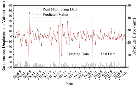
Figure 10.
Predicted and monitored random displacement components.
3.3.4. Result of Cumulative Displacement
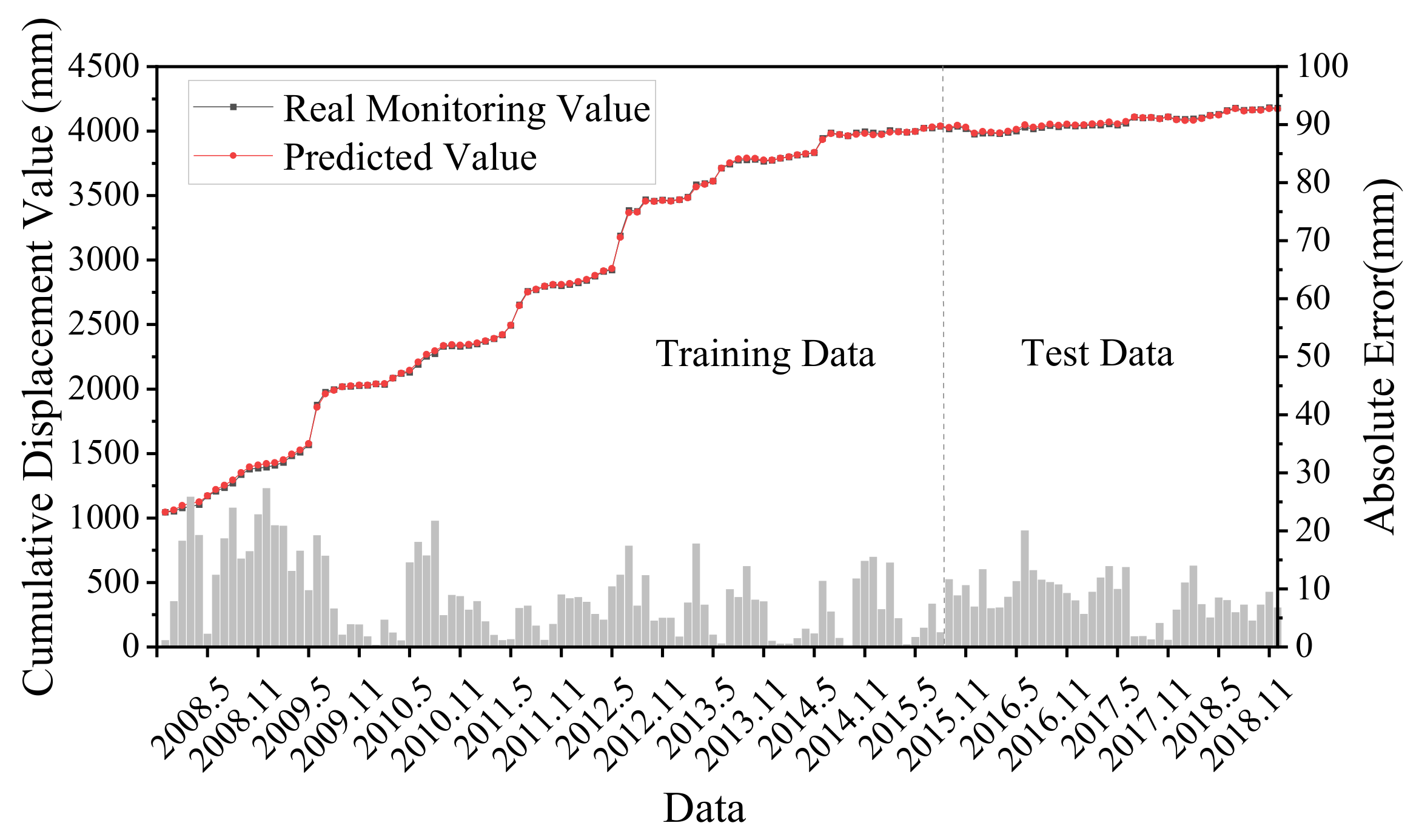
According to the principle of time series decomposition, the predicted displacement values of trend item, periodic item and random item obtained by the LSTM model were superimposed to obtain the predicted cumulative total displacement of the Shuping landslide. The cumulative landslide displacement prediction results and errors obtained by superposition are shown in Figure 11. The R2 of the prediction result was 0.970, which is a good fit between the predicted and real values and captures the increasing trend of landslide displacement well. The MAE of the prediction result was 8.58 mm, and the RMSE was 9.60 mm, which generally has a high prediction accuracy and can better reflect the step-type characteristics of the landslide.
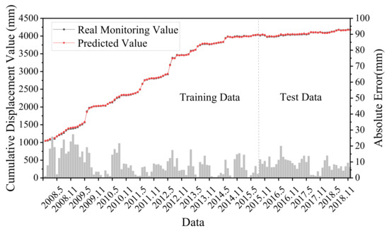
Figure 11.
Predicted and monitored cumulative displacement components.
4. Discussion
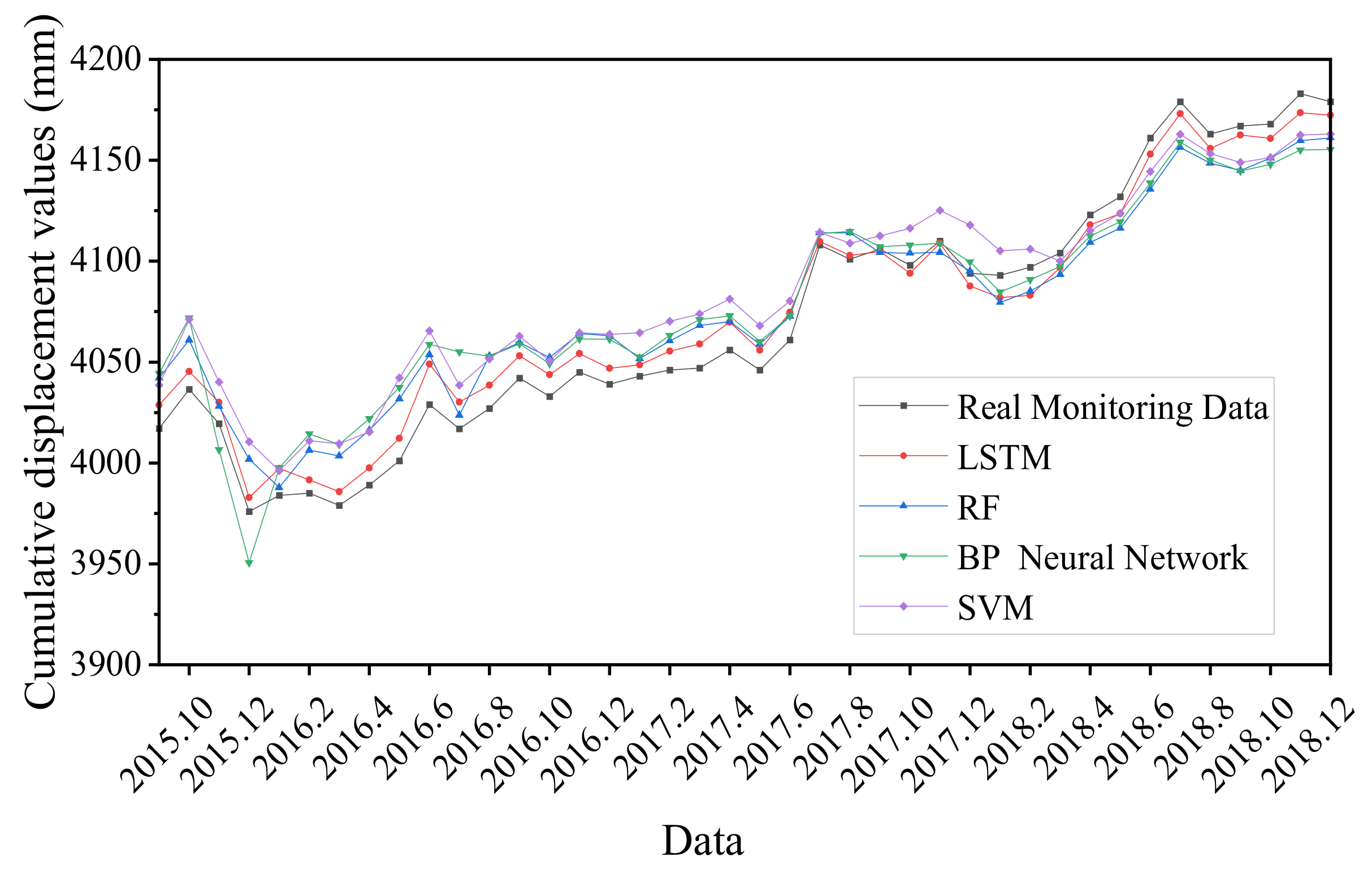
To further assess the prediction advantage of the LSTM model over traditional machine learning methods, the prediction results of random forest (RF), BP neural network and SVM were compared and analyzed with the prediction results on the test set of the model. The prediction results of each model are shown in Figure 12. Overall, all four models fit the trend of landslide displacement monitoring signals, but in comparison, the LSTM model was closer to the real values of the monitoring sites and has a higher degree of fitting. The main reason is that LSTM uses historical data information to predict the displacement at the current location, linking independent displacement data; the model fully selects and learns the information in historical displacement based on the “gate” structure, and continuously updates the learned experience for the current prediction task.
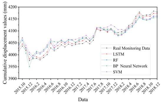
Figure 12.
Comparison of cumulative displacements of different models.
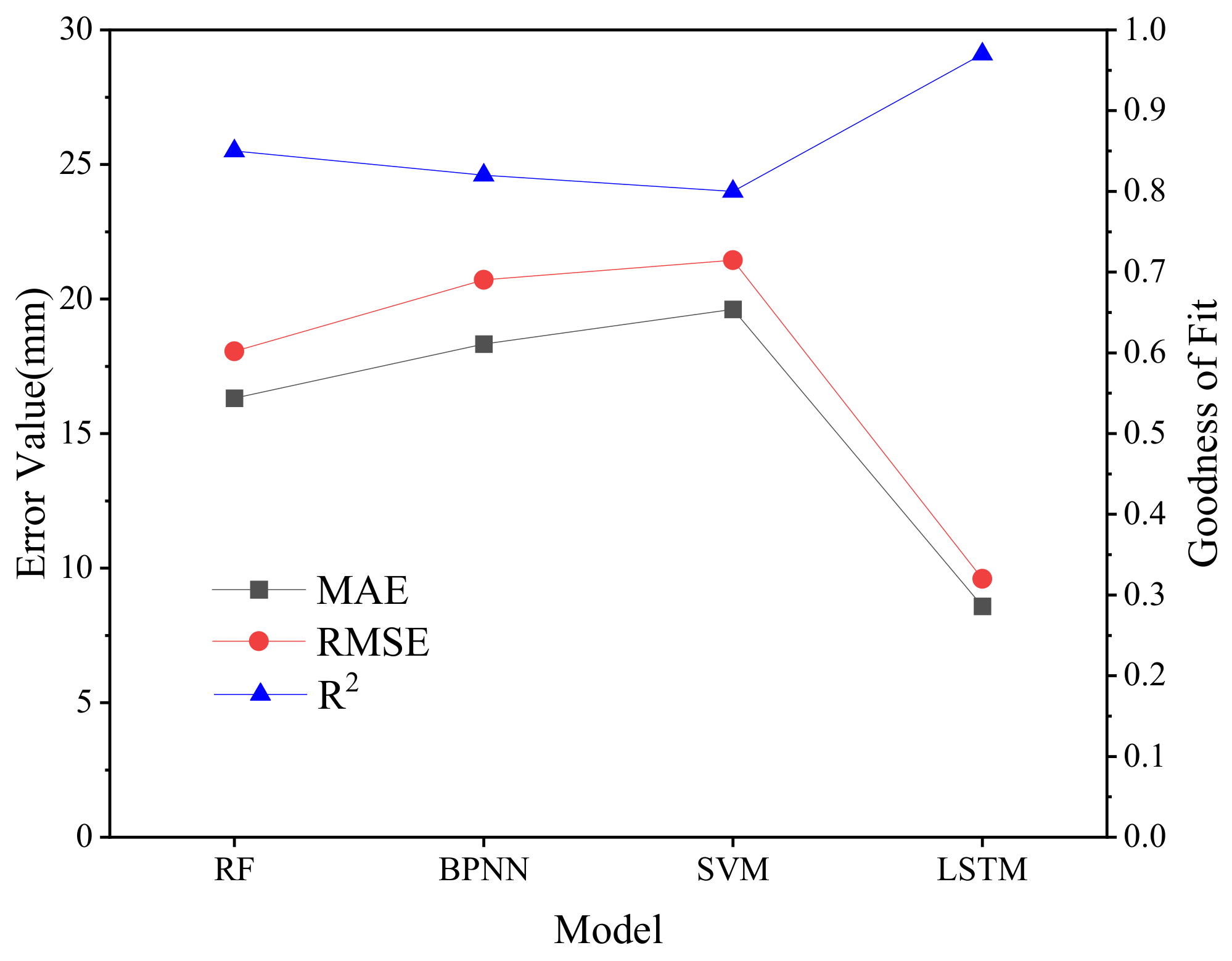
From the model evaluation index, the smaller error index and higher fitting degree were the desired results. The results were shown in Figure 13. For the prediction error, the average absolute error and root mean square error of the LSTM model were smaller than the other three models, and the predicted value was closer to the real value. For the goodness of fit, the LSTM model reached 0.97, and the RF, BP neural network and SVM models were 0.85, 0.82 and 0.80, respectively. Overall, compared with the traditional machine learning methods, the LSTM model takes into account the influence of the time factor, has better prediction results and stronger generalization ability and the overall trend can be captured for the unknown dataset.
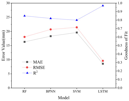
Figure 13.
Comparison of predictive model evaluation indicators.
5. Conclusions
The landslide deformation of the reservoir bank is affected by the reservoir water level, rainfall and other cyclical factors, and its displacement curve is characterized by a step-like feature. Aiming at the shortcomings of most landslide displacement prediction models that ignore random displacement, this paper proposes a landslide displacement prediction model based on the SSA-VMD decomposition algorithm and LSTM algorithm. Firstly, the VMD algorithm is used to decompose the nonlinear data series of landslide cumulative displacements into trend terms, period terms and random terms with corresponding characteristics. In order to improve the effectiveness of the decomposition results, the SSA algorithm is used to solve the model parameters of the VMD so that the optimal parameters replace the initial parameters. Then, the correlation between the influencing factors such as reservoir level and rainfall and the subsequence of the period term is analyzed and the correlation between them is quantified to determine the input characteristics of the prediction model. According to the change characteristics of landslide displacement, the sub-items of landslide displacement are predicted separately using the LSTM model, and the prediction results are summed up to obtain the prediction results of cumulative displacement. The real landslide dataset of the Shuping landslide in Three Gorges Reservoir Area, China is utilized for validation, and good results are achieved. The final results show that the SSA-VMD model coupled with the LSTM model proposed in this paper can predict the landslide displacement more accurately. In the future, the model will be improved according to the different characteristics of landslides and promoted to be applied to the displacement prediction of other landslides. In addition, the model can also be applied to other signal decomposition and time series prediction fields to help decision makers continuously optimize the decision-making process.
Author Contributions
Conceptualization, X.X. and Y.H.; methodology, X.X.; formal analysis, Y.H.; resources, Y.H.; writing—original draft preparation, X.X. and Y.H.; writing—review and editing, X.X. and Y.H.; visualization, Y.H. All authors have read and agreed to the published version of the manuscript.
Funding
This research received no external funding.
Data Availability Statement
Restrictions apply to the availability of the data. Data were obtained from the National Cryosphere Desert Data Center/National Service Center for the Speciality Environment Observation Station.
Conflicts of Interest
The authors declare no conflicts of interest.
References
- Depina, I.; Oguz, E.A.; Thakur, V. Novel Bayesian framework for calibration of spatially distributed physical-based landslide prediction models. Comput. Geotech. 2020, 125, 103660. [Google Scholar] [CrossRef]
- Li, S.H.; Wu, L.Z.; Chen, J.J.; Huang, R.Q. Multiple data-driven approach for predicting landslide deformation. Landslides 2020, 17, 709–718. [Google Scholar] [CrossRef]
- Wang, C.H.; Zhao, Y.J. Time Series Prediction Model of Landslide Displacement Using Mean-Based Low-Rank Autoregressive Tensor Completion. Appl. Sci. 2023, 13, 5214. [Google Scholar] [CrossRef]
- Liu, Z.Q.; Guo, D.; Lacasse, S.; Li, J.H.; Yang, B.B.; Choi, J.C. Algorithms for intelligent prediction of landslide displacements. J. Zhejiang Univ.-Sci. A 2020, 21, 412–429. [Google Scholar] [CrossRef]
- Huang, F.M.; Ye, Z.; Jiang, S.H.; Huang, J.S.; Chang, Z.L.; Chen, J.W. Uncertainty study of landslide susceptibility prediction considering the different attribute interval numbers of environmental factors and different data-based models. Catena 2021, 202, 105250. [Google Scholar] [CrossRef]
- Jiang, Y.N.; Xu, Q.; Lu, Z.; Luo, H.Y.; Liao, L.; Dong, X.J. Modelling and predicting landslide displacements and uncertainties by multiple machine-learning algorithms: Application to Baishuihe landslide in Three Gorges Reservoir, China. Geomat. Nat. Hazards Risk 2021, 12, 741–762. [Google Scholar] [CrossRef]
- Saito, M. Forecasting the time of occurrence of a slope failure. In Proceedings of the International Conference on Soil Mechanics and Foundation Engineering, Montreal, QC, Canada, 8–15 September 1965; pp. 537–541. [Google Scholar]
- Mufundirwa, A.; Fujii, Y.; Kodama, J. A new practical method for prediction of geomechanical failure-time. Int. J. Rock Mech. Min. Sci. 2010, 47, 1079–1090. [Google Scholar] [CrossRef]
- Helmstetter, A.; Sornette, D.; Grasso, J.R.; Andersen, J.V.; Gluzman, S.; Pisarenko, V. Slider block friction model for landslides: Application to Vaiont and La Clapiere landslides. J. Geophys. Res. Solid Earth 2004, 109. [Google Scholar] [CrossRef]
- Cascini, L.; Scoppettuolo, M.R.; Babilio, E. Forecasting the landslide evolution: From theory to practice. Landslides 2022, 19, 2839–2851. [Google Scholar] [CrossRef]
- Miao, S.J.; Hao, X.; Guo, X.L.; Wang, Z.M.; Liang, M.C. Displacement and landslide forecast based on an improved version of Saito’s method together with the Verhulst-Grey model. Arab. J. Geosci. 2017, 10, 53. [Google Scholar] [CrossRef]
- Liu, L.L.; Yin, H.D.; Xiao, T.; Huang, L.; Cheng, Y.M. Dynamic prediction of landslide life expectancy using ensemble system incorporating classical prediction models and machine learning. Geosci. Front. 2024, 15, 101758. [Google Scholar] [CrossRef]
- Wu, L.Z.; Li, S.H.; Huang, R.Q.; Xu, Q. A new grey prediction model and its application to predicting landslide displacement. Appl. Soft Comput. 2020, 95, 106543. [Google Scholar] [CrossRef]
- Li, S.H.; Zhu, L.; Wu, Y.; Lei, X.Q. A novel grey multivariate model for forecasting landslide displacement. Eng. Appl. Artif. Intell. 2021, 103, 104297. [Google Scholar] [CrossRef]
- Wang, Y.K.; Tang, H.M.; Wen, T.; Ma, J.W. A hybrid intelligent approach for constructing landslide displacement prediction intervals. Appl. Soft Comput. 2019, 81, 105506. [Google Scholar] [CrossRef]
- Huang, F.M.; Yin, K.L.; Zhang, G.R.; Gui, L.; Yang, B.B.; Liu, L. Landslide displacement prediction using discrete wavelet transform and extreme learning machine based on chaos theory. Environ. Earth Sci. 2016, 75, 1376. [Google Scholar] [CrossRef]
- Zhang, L.G.; Chen, X.Q.; Zhang, Y.G.; Wu, F.W.; Chen, F.; Wang, W.T.; Guo, F. Application of GWO-ELM Model to Prediction of Caojiatuo Landslide Displacement in the Three Gorge Reservoir Area. Water 2020, 12, 1860. [Google Scholar] [CrossRef]
- Zhou, C.; Yin, K.L.; Cao, Y.; Intrieri, E.; Ahmed, B.; Catani, F. Displacement prediction of step-like landslide by applying a novel kernel extreme learning machine method. Landslides 2018, 15, 2211–2225. [Google Scholar] [CrossRef]
- Li, Y.Y.; Sun, R.L.; Yin, K.L.; Xu, Y.; Chai, B.; Xiao, L.L. Forecasting of landslide displacements using a chaos theory based wavelet analysis-Volterra filter model. Sci. Rep. 2019, 9, 19853. [Google Scholar] [CrossRef] [PubMed]
- Meng, Y.D.; Qi, Y.; Cai, Z.L.; Tian, B.; Yuan, C.W.; Zhang, X.Y.; Zuo, Q.J. Dynamic forecast model for landslide displacement with step-like deformation by applying GRU with EMD and error correction. Bull. Eng. Geol. Environ. 2023, 82, 211. [Google Scholar] [CrossRef]
- Shihabudheen, K.V.; Peethambaran, B. Landslide displacement prediction technique using improved neuro-fuzzy system. Arab. J. Geosci. 2017, 10, 502. [Google Scholar] [CrossRef]
- Niu, X.X.; Ma, J.W.; Wang, Y.K.; Zhang, J.R.; Chen, H.J.; Tang, H.M. A Novel Decomposition-Ensemble Learning Model Based on Ensemble Empirical Mode Decomposition and Recurrent Neural Network for Landslide Displacement Prediction. Appl. Sci. 2021, 11, 4684. [Google Scholar] [CrossRef]
- Yao, H.Y.; Song, G.L.; Li, Y.B. Displacement Prediction of Channel Slope Based on EEMD-IESSA-LSSVM Combined Algorithm. Appl. Sci. 2023, 13, 9582. [Google Scholar] [CrossRef]
- Bai, D.X.; Lu, G.Y.; Zhu, Z.Q.; Tang, J.T.; Fang, J.; Wen, A.X. Using time series analysis and dual-stage attention-based recurrent neural network to predict landslide displacement. Environ. Earth Sci. 2022, 81, 509. [Google Scholar] [CrossRef]
- Guo, W.; Meng, Q.J.; Wang, X.; Zhang, Z.T.; Yang, K.; Wang, C.H. Landslide Displacement Prediction Based on Variational Mode Decomposition and GA-Elman Model. Appl. Sci. 2023, 13, 450. [Google Scholar] [CrossRef]
- Qi, Y.L.; Bai, L.; Hou, T.; Huang, P.P.; Tan, W.X.; Xu, W. Application of Displacement Prediction Method Based on Displacement Increment and CS-BP Neural Network in Mine Landslide. Prog. Electromagn. Res. Lett. 2023, 113, 69–79. [Google Scholar] [CrossRef]
- Wang, G.; Fang, Z.; Xie, J.R.; Du, N. Development of a Hybrid Method to Predict the Slope Surface Deformation Utilizing the Time Series and GA-Elman Models. Adv. Civ. Eng. 2021, 2021, 6642456. [Google Scholar] [CrossRef]
- Li, L.M.; Cheng, S.K.; Wen, Z.Z. Landslide prediction based on improved principal component analysis and mixed kernel function least squares support vector regression model. J. Mt. Sci. 2021, 18, 2130–2142. [Google Scholar] [CrossRef]
- Zhou, S.T.; Yao, Y.K.; Luo, X.D.; Jiang, N.; Niu, S.S. Dynamic Response Evaluation for Single-Hole Bench Carbon Dioxide Blasting Based on the Novel SSA-VMD-PCC Method. Int. J. Geomech. 2023, 23, 04022248. [Google Scholar] [CrossRef]
- Li, Y.; Fu, P.; Ji, W.F.; Shi, S.W.; Zhang, Y.; Zhang, T. Predictive method of nonlinear system based on artificial neural network and SVM. Oxid. Commun. 2016, 39, 1226–1235. [Google Scholar]
- Zhou, C.; Yin, K.L.; Cao, Y.; Ahmed, B. Application of time series analysis and PSO-SVM model in predicting the Bazimen landslide in the Three Gorges Reservoir, China. Eng. Geol. 2016, 204, 108–120. [Google Scholar] [CrossRef]
- Guo, Z.Z.; Chen, L.X.; Gui, L.; Du, J.; Yin, K.L.; Do, H.M. Landslide displacement prediction based on variational mode decomposition and WA-GWO-BP model. Landslides 2020, 17, 567–583. [Google Scholar] [CrossRef]
- Miao, F.S.; Wu, Y.P.; Xie, Y.H.; Li, Y.N. Prediction of landslide displacement with step-like behavior based on multialgorithm optimization and a support vector regression model. Landslides 2018, 15, 475–488. [Google Scholar] [CrossRef]
- Lin, Z.; Ji, Y.F.; Liang, W.B.; Sun, X.Y. Landslide Displacement Prediction Based on Time-Frequency Analysis and LMD-BiLSTM Model. Mathematics 2022, 10, 2203. [Google Scholar] [CrossRef]
- Lin, Z.A.; Sun, X.Y.; Ji, Y.F. Landslide Displacement Prediction Model Using Time Series Analysis Method and Modified LSTM Model. Electronics 2022, 11, 1519. [Google Scholar] [CrossRef]
- Dragomiretskiy, K.; Zosso, D. Variational Mode Decomposition. IEEE Trans. Signal Process. 2014, 62, 531–544. [Google Scholar] [CrossRef]
- Tang, A.D.; Zhou, H.; Han, T.; Xie, L. A Chaos Sparrow Search Algorithm with Logarithmic Spiral and Adaptive Step for Engineering Problems. Cmes-Comput. Model. Eng. Sci. 2022, 130, 331–364. [Google Scholar] [CrossRef]
- Wu, L.M.; Wang, Z. Three Gorges Reservoir Water Level Fluctuation Influents on the Stability of the Slope’s Analysis. Adv. Mater. Res. 2013, 739, 283–286. [Google Scholar] [CrossRef]
- He, K.Q.; Zhao, M.; Zhang, Y.J.; Zhang, J.X. Unload-load displacement response ratio parameter and its application in prediction of debris landslide induced by rainfall. Environ. Earth Sci. 2017, 76, 55. [Google Scholar] [CrossRef]
- Du, J.; Yin, K.L.; Lacasse, S. Displacement prediction in colluvial landslides, Three Gorges Reservoir, China. Landslides 2013, 10, 203–218. [Google Scholar] [CrossRef]
Disclaimer/Publisher’s Note: The statements, opinions and data contained in all publications are solely those of the individual author(s) and contributor(s) and not of MDPI and/or the editor(s). MDPI and/or the editor(s) disclaim responsibility for any injury to people or property resulting from any ideas, methods, instructions or products referred to in the content. |
© 2024 by the authors. Licensee MDPI, Basel, Switzerland. This article is an open access article distributed under the terms and conditions of the Creative Commons Attribution (CC BY) license (https://creativecommons.org/licenses/by/4.0/).

