Transformer-Based Parameter Estimation in Statistics

Abstract

Parameter estimation is one of the most important tasks in statistics, and is key to helping people understand the distribution behind a sample of observations. Traditionally, parameter estimation is done either by closed-form solutions (e.g., maximum likelihood estimation for Gaussian distribution) or by iterative numerical methods such as the Newton–Raphson method when a closed-form solution does not exist (e.g., for Beta distribution). In this paper, we propose a transformer-based approach to parameter estimation. Compared with existing solutions, our approach does not require a closed-form solution or any mathematical derivations. It does not even require knowing the probability density function, which is needed by numerical methods. After the transformer model is trained, only a single inference is needed to estimate the parameters of the underlying distribution based on a sample of observations. In the empirical study, we compared our approach with maximum likelihood estimation on commonly used distributions such as normal distribution, exponential distribution and beta distribution. It is shown that our approach achieves similar or better accuracy as measured by mean-square-errors.

1. Introduction

Parameter estimation is one of the most important tasks in statistics. Given the type of the underlying distribution and a sample of observations, a parameter estimation method should produce an estimate of the distribution’s parameters. Taking 1-dimensional normal distribution as an example. Given a sample $x_1$, …, $x_N$ drawn from normal distribution $\mathcal{N}(\mu ,{\sigma }^2)$, we hope to estimate its parameters $\mathsf{\mu }$ and $\sigma$. The most commonly used method is MLE (maximum likelihood estimation). It can be easily proven that the MLE of $\mathsf{\mu }$ is $\widehat{\mu }=\frac{{\sum }_{i=1}^N{x}_i}{N}$, and that of $\sigma$ is $\widehat{\sigma }=\sqrt{\frac{{\sum }_{i=1}^N(x_i-\widehat{\mu }{)}^2}{N}}$. The proof can be found in [1].

Parameter estimation for some other distributions can be much more complex. For example, it is shown that the maximum likelihood estimation for the parameters of a Beta distribution has no closed form [2], and one needs to resort to numeric optimization methods such as the Newton–Raphson method or gradient descent to estimate its parameters.

In recent years, transformers [3] has become the state-of-the-art for both natural language processing and computer vision, and large transformer-based models (such as GPT) are capable of solving challenging problems in many areas including math and programming. On the other hand, transformer-based approaches have been successfully applied to many diverse tasks, including many mathematical tasks such as solving word problems [4], mathematical reasoning [5], symbolic regressions [6], and time-series forecasting [7]. In this paper, we propose an approach to perform parameter estimation using deep learning. For each type of distribution, we generate a training set, with each training example containing a sample drawn from a distribution with predetermined parameters. Then, we convert each sample into a sequence of embeddings, and train a transformer to predict the parameter(s) with the sequence being the input. We aim at producing estimations that are as close as possible to the true parameters, i.e., we are making mean-square-error estimations of the parameters.

The advantage of our approach is that it does not require any mathematical derivation. Thus, the mathematical complexity of the probability density function does not pose any burden for the transformer model, even though there may not be any closed-form solutions to MLE for the parameters for the distribution. Iterative methods (such as the Newton–Raphson method or gradient descent) have been used for estimating the parameters for a distribution when there is no closed-form solution (e.g., [8]). Compared to such methods, our approach has two advantages. Firstly, our approach is not iterative and just requires a single inference of a transformer model. Secondly, and more importantly, our approach does not even require knowing the probability density function of the distribution. For example, suppose a manufacturer is testing the percentage of two materials in electrical filaments in bulbs. The life of a bulb follows a distribution with a single parameter which is the percentage of the first material. Even if the distribution is unknown to us, we can still learn to estimate the parameter from many samples of bulb lives. Another example is that when testing the hyperparameters of a particular deep learning model, the prediction error on a random test case follows a distribution that is unknown to us. However, we can estimate the hyperparameters based on samples of such errors.

In general, we make the following contributions in this paper:

• We present a novel approach to using transformers for parameter estimation.
• We propose a way to convert a sample of a distribution into a sequence of embeddings, which can be easily consumed by a transformer and can carry precise information about the sample.
• We conduct a comprehensive empirical study, which compares our approach with maximum likelihood estimation methods for various distributions.
• It is shown that when measured by mean-square-error (MSE), our approach outperforms MLE in most commonly used distributions such as normal distribution and exponential distribution. Please note that this does not indicate MLE is not a good method, as it always maximizes the probability of observing a sample. Our experiment simply indicates that our method outperforms MLE in terms of mean-square-error in most scenarios, which is a common way to evaluate a method of parameter estimation.

The rest of the paper is organized as follows. Related work is presented in Section 2. Section 3 describes our approach for parameter estimation with a transformer. Experimental results are reported in Section 4 and Section 5 concludes this paper.

2. Related Work

In recent years, there have been many studies that successfully applied transformer-based approaches to a diverse set of math tasks, including solving word problems [4], mathematical reasoning [5], symbolic regressions [6], and time-series forecasting [7].

Ref. [9] discusses methods for using machine learning and deep neural networks for various parameter estimation tasks. In recent years, transformer-based approaches demonstrated superior performances than traditional deep neural nets in various applications, such as natural language processing and computer vision. Large language models, such as GPT and Gemini, have become assistants for all kinds of tasks from make spreadsheets to writing computer programs, and have shown early signs of general AI. Therefore, in this paper, we study the usage of a transformer-based approach on parameter estimation. We show that a random sample can be easily encoded as embeddings which are inputs to a transformer, and thus a transformer model can naturally be used for parameter estimation in statistics.

In [10], the authors proposed an EM-based method for estimating parameters of a Trapezoidal beta distribution. In [11], a method was proposed to convert Bayesian parameter estimation as a classification problem, which was then solved using a multi-layer perceptron network. This approach is very useful in determining if the sample was drawn from a distribution with a particular set of predetermined parameters, but it is not capable of performing parameter estimation, as it requires a hypothesis of what the parameters are.

Deep learning has been used to estimate the parameters in various applications other than statistics. In [12], the authors proposed a method to use CNN to estimate the parameters of events based on LIGO data. [13] describes a method to estimate Magnetic Hamiltonian parameter from electron microscopy images using CNN. In [14], the authors used GRU for parameter estimation of MRI with an application in pancreatic cancer.

Our work is different from the above in several aspects: (1) We study the problem of parameter estimation in statistics, which is key to understanding the underlying distribution of data. (2) We use transformer, which has become the state-of-the-art in most of the important applications including both NLP and computer vision. (3) Unlike the above work which uses the raw data of a specific problem as the input to their deep learning models, we convert a sample of an arbitrary distribution into a sequence of embeddings, which can be consumed by a transformer.

3. Parameter Estimation Using Transformer

3.1. Problem Definition

Our goal is to train a model that can predict the parameters of a distribution, using a sample drawn from it. Let us take normal distribution as an example. A normal distribution $\mathcal{N}(\mu ,{\sigma }^2)$ has two parameters $\mathsf{\mu }$ and $\sigma$, and its probability density function is p(x) = $\frac{1}{\sigma \sqrt{2\pi }}$$exp(-\frac{1}{2}{\left(\frac{x-\mu }{\sigma }\right)}^2)$. Given a sample $x_1$, …, $x_N$, the maximum likelihood estimator of $\mathsf{\mu }$ is just the sample mean $\frac{{\sum }_{i=1}^N{x}_i}{N}$. The MLE for $\sigma$ is $\sqrt{\frac{{\sum }_{i=1}^N(x_i-\widehat{\mu }{)}^2}{N}}$.

We will train a model to predict the two parameters $\mathsf{\mu }$ and $\sigma$, using a random sample drawn from the distribution as the model’s input. The model will be trained on a large number of samples, each from a different normal distribution with different parameters. In this paper, we use the loss function of mean-square-error, and will evaluate the accuracy of our model by the mean-square-error of its predictions.

In this paper, we only study univariate distributions, although our method can be easily extended to multivariate distributions.

3.2. Data Normalization

Some distributions can be shifted and stretched along the x-axis (e.g., normal distribution), simply by replacing x with another variable $x^{\prime }=\beta (x-\alpha )$. Therefore, given a data sample, we first normalize the range to $[0,1]$, which can be easily converted into a sequence of tokens, as described later in this section. After the model makes a prediction, the predicted parameters can be easily converted back. For example, if we replace x with $x^{\prime }=\beta (x-\alpha )$ during normalization and then predict the parameters of a normal distribution to be ${\mu }^{\prime }$ and ${\sigma }^{\prime }$, then our predicted parameters are actually $\widehat{\mu }=\frac{{\mu }^{\prime }}{\beta }+\alpha$, and $\widehat{\sigma }=\frac{{\sigma }^{\prime }}{\beta }$.

Unlike normal distribution, some distributions can only be stretched along the x-axis, but cannot be shifted, such as exponential distribution. For such distributions, we also normalize the range of each sample to $[0,1]$, and again the estimated parameters can be easily converted back.

3.3. Data Representation

The input to a transformer [3] is a sequence of embeddings, each being a vector of a fixed number of dimensions. Suppose we use a transformer that takes at most L input embeddings, with embedding size being K. We use each value in each embedding to represent a possible value. For example, if $L=1024$ and $K=384$, we can represent $384\times 1024=393,216$ different values. We tried two ways to represent a value:

• Seq-first: First, divide the range of $[0,1]$ into L intervals, each corresponding to an embedding in our sequence of length L. Then, divide each of the L intervals into K sub-intervals, each represented by one dimension of the embedding.
• Embed-first: First, divide the range of $[0,1]$ into K intervals, each corresponding to a particular dimension in all the L positions. Then, divide each of the K intervals into L sub-intervals, to determine which position it should reside in.

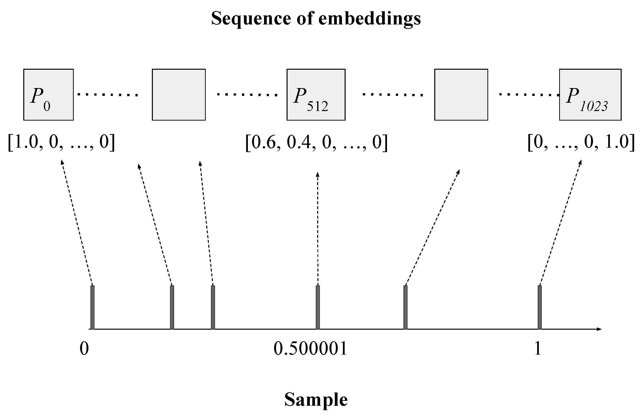
Figure 1 illustrates how Seq-first conversion is done. We first divide the range $[0,1]$ into 1024 intervals, and then each interval into 384 sub-intervals. The sample on the horizontal axis contains six observations. The leftmost observation is mapped to the first dimension of the first embedding. The observation 0.500001 maps to somewhere between the first and second dimensions of the 512th embedding. The first dimension of the 512th embedding maps to interval $[0.5,0.5000025]$, and the second dimension maps to interval $[0.5000025,0.500005]$. The observation 0.500001 falls into the interval of the first dimension. Instead of assigning all its weight to the first dimension, we assign part of its weight to the second dimension, according to its position in the first dimension’s interval, so that we can precisely represent where the observation is. In this case, the observation appears at the 40-percentile position of the first interval, and thus we keep 60% of its weight in the first dimension, and move 40% of its weight to the second dimension.

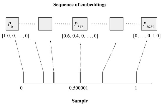
Figure 1. Converting a sample into a sequence of L embeddings ($L=1024$), each of size K ($K=384$). The sample contains 6 observations, ranging from 0 to 1 (after normalization). The left-most observation is mapped to the first dimension of the first embedding. The rightmost observation is mapped to the last dimension of the last embedding. The observation 0.500001 maps to somewhere between the first and second dimensions of the 512th embedding, and thus its weight is distributed between these two dimensions.

If we use the Embed-first representation, we assign an observation’s weight to the same dimension in two different positions, in a similar way as the Seq-first representation.

3.4. Transformer Model

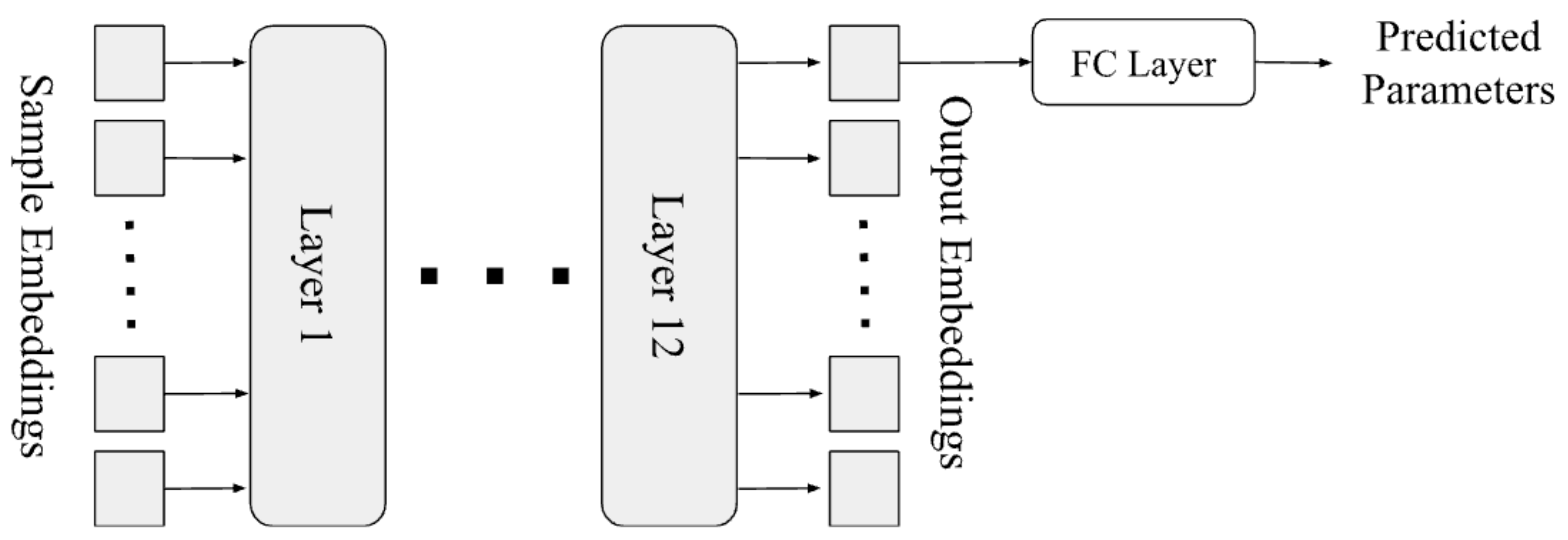
As shown in Figure 2, our model is a typical transformer [3], which takes the sequence of embeddings as its input, and outputs the predicted parameter(s), by adding an output layer on top of the first output embedding of the last layer in the transformer. Since this is a regression problem, we define the loss function as the average mean-square-error on each parameter to be predicted.

Figure 2. Architecture of our transformer model.

Each training example is a sample drawn from a distribution with random parameters. Therefore, our model should never see the same example twice during training. If the sample has been stretched or shifted as described in Section 3.2, we first convert the predicted parameters back to the original scale, and then compare them to the true parameters of the distribution for loss computation. If there are multiple parameters, we use the average mean-square-error between predicted parameter values and their true values as the loss.

4. Experiments

4.1. Experiment Settings

We test our approach on three types of commonly seen distributions: Normal distributions, exponential distributions, and Poisson distributions. The training and testing data are randomly generated as needed, and thus the model should never see the same example twice. We use the RoBERTa model [15] downloaded from Huggingface as our transformer model. RoBERTa is a variation of BERT [16] with various optimizations such as adjusted batch sizes and learning rate.

All experiments are done on a machine with an A6000 GPU, with Ubuntu 18.04, CUDA 11.7 and Pytorch 2.0.0. Float32 is used because numerical precision is key to our approach.

Unless otherwise mentioned, we train our model on 9.9M randomly generated examples in each setting, and test its accuracy on 100K examples. We choose our hyperparameters for efficiency reasons, and the hyperparameters chosen have negligible difference in accuracy compared with the default hyperparameters of RoBERTa. The training usually takes 60–70 h using the default setting. Please note that for each type of distribution we only need to train once, and 60–70 h of machine time is negligible to the time consumed by a human to derive the formula or algorithm for parameter estimation.

Transformer Hyperparameters

We first test various hyperparameters for our transformer model, in order to select the best settings. We start with the open-sourced RoBERTa, which accepts 512 embeddings as its input, each having 768 dimensions. In order to increase the precision, we tried to increase input length to 1024, which quadruples the memory consumption for multihead-self-attention. Due to the limitation of our GPU memory, we had to change the number of layers from 12 to 6, and embedding size from 768 to 384. As discussed in Section 3.3, we use Seq-first by default, and tried Embed-first as well.

We use each of the above methods to estimate the parameters for normal distributions, with 9.9 M samples (of size 30) for training, and 100 K samples for testing. More details are described in Section 4.3.1. The results are shown in Table 1. We can see RoBERTa and RoBERTa with 1024-input-len have very similar accuracies. A t-test shows there is no statistically significant difference between their MSEs. We choose RoBERTa with 1024-input-len because its training time is much lower.

Table 1. Mean-square-error and training time of various settings for normal distribution.

	MSE	Training Time	Avg. Inference Time
RoBERTa	0.7215	91 h 43 min	12.7 ms
RoBERTa 1024-input-len	0.7169	63 h 35 min	23.6 ms
RoBERTa 1024-input-len Embed-first	3.155	63 h 24 min	22.7 ms
Maximum likelihood estimation	0.8056	N/A	<5 ms

Although it takes tens of hours to train a model for parameter estimation for a particular type of distributions, the actual parameter estimation can be done within 25 ms. Once the model is trained, we only need to feed in a sample from a distribution, which will be converted into a sequence of embeddings and fed into the model. RoBERTa can usually finish the inference and produce outputs in 10–20 ms. Please note that we do not even need to know the probability density function of the underlying distribution in order to train and use such a model.

4.2. Exponential Distribution

We start from exponential distribution because of its simplicity. We represent the p.d.f. of exponential distribution in the same way as NumPy (https://numpy.org/doc/stable/reference/random/generated/numpy.random.exponential.html, accessed on 18 August 2023):

$$f(x;\beta )=\frac{1}{\beta }exp(-\frac{x}{\beta }),wherex>0,\beta >0$$

(1)

Here $\beta$ is the only parameter and represents the scale of the distribution. It is equivalent to the alternative p.d.f. $f(x;\lambda )=\lambda e^{-\lambda x}$, where $\lambda =\frac{1}{\beta }$. When generating samples, we take $\beta$ from a uniform distribution in range [0.5, 2].

We test our approach and maximum likelihood estimation on 100K samples, and the average mean-square-error is recorded. Each approach is tested in two settings:

• Known Parameter Range: The range of each parameter is known to the approach.
• Unknown Parameter Range: The approach is not aware of the range of any parameter.

4.2.1. Known Parameter Range

When each parameter’s range is known, we normalize each sample into [0, 1] by a fixed linear transform. When $\beta \in [0.5,2]$, the probability of $x>20$ is less than 0.5%. Therefore, we cap each value of a sample within [0, 20], and normalize each capped value $x_i$ by ${x_i}^{\prime }=x_i/20$. In the final fully-connected layer for predicting parameters (as in Figure 2), we let it directly predict the value of the parameter.

The MLE of $\beta$ is simply $\frac{{\sum }_{i=1}^N{x}_i}{N}$, and we cap its estimate of $\beta$ within [0.5, 2].

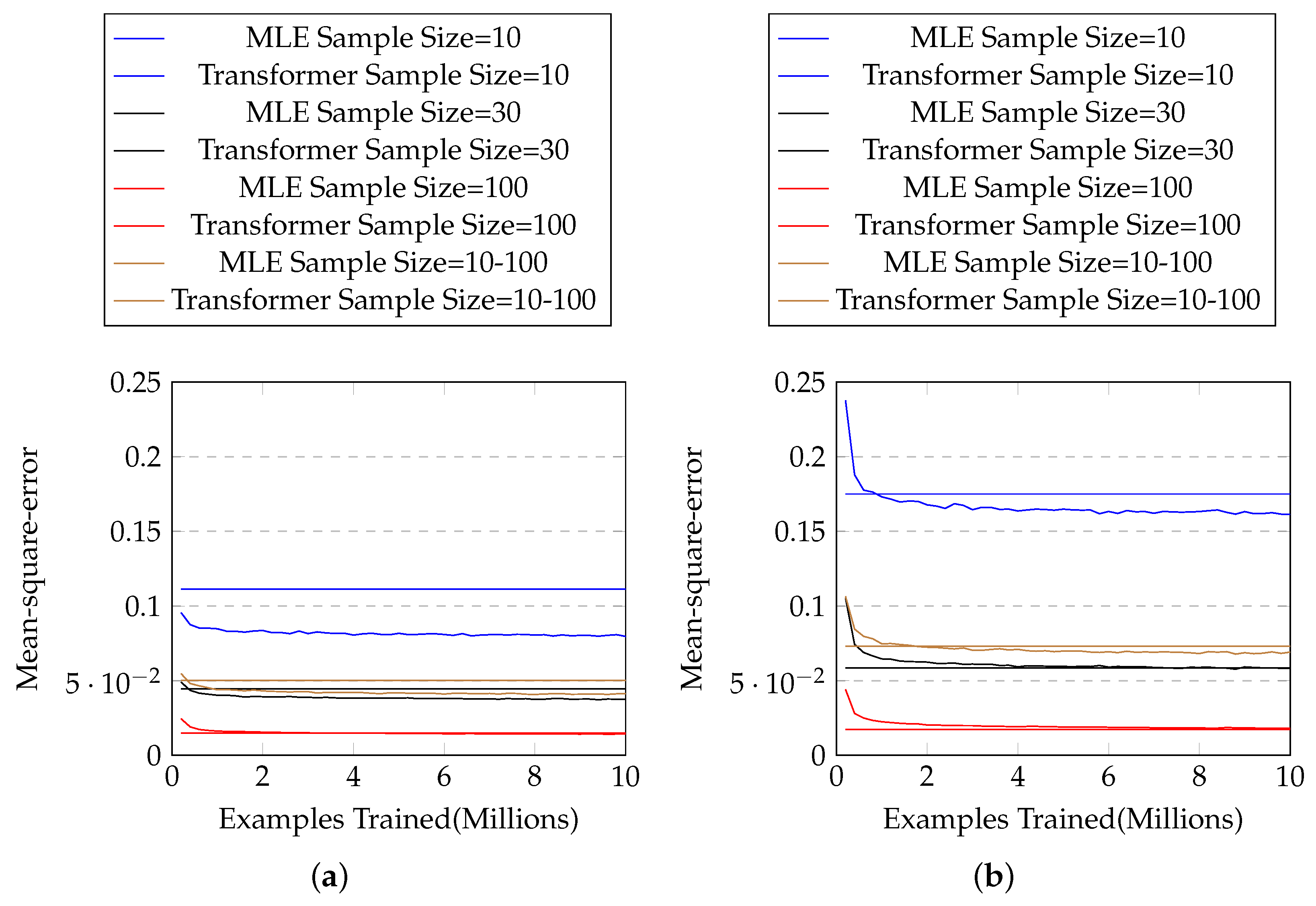
We test with three different sample sizes (10, 30, and 100), and another setting in which the sample size is randomly sampled from a log-uniform distribution of range [10, 100]. The results are shown in Figure 3a, in which our method outperforms MLE for each sample size. Table 2 shows the mean and standard deviation of the mean-square-error of the two approaches for each sample size. One can see that our proposed approach solidly beats MLE in every sample size, with close to zero p-values in two-sample t-tests.

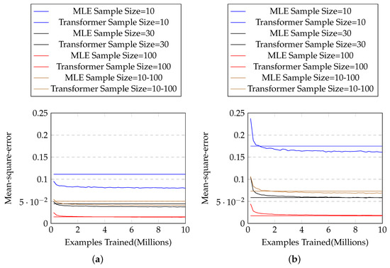
Figure 3. (a) The mean-square-error with # training examples for exponential distributions with known parameter ranges. The horizontal lines represent mean-square-errors of MLE, and the curves represent those of our approach. (b) Those for exponential distributions with unknown parameter ranges.

Table 2. The mean-square-error of MLE and our approach for each sample size for exponential distribution with known parameter range, together two-sample t-test results.

Sample Size	MLE (Mean/Std)	Our Approach (Mean/Std)	t-Value	p-Value
10	0.1113/0.1726	0.0796/0.1168	48.101	0.0001
30	0.0445/0.0727	0.0375/0.0631	22.995	0.0001
100	0.0149/0.0250	0.0143/0.0222	6.4316	0.0001
10 to 100	0.0503/0.0949	0.0413/0.0751	23.517	0.0001

4.2.2. Unknown Parameter Range

Suppose a sample is drawn from an exponential distribution $exp\left(\beta \right)$, and the range of $\beta$ is unknown to the method for parameter estimation (i.e., the method needs to assume that $\beta$ can take any value). For MLE, we can simply use its formula (as in Section 4.2.1) to estimate the parameters. But a slightly more complex method is needed for our approach.

In order to hide the parameter’s range from our transformer model, we first normalize each sample s into range $[0,1]$. Let $b=max\left(s\right)$. Each value $x_i$ is normalized by ${x_i}^{\prime }=x_i/b$. In this way our model can only see the relative shape of the sample, without knowing its original range. Suppose the model’s prediction is ${\beta }^{*}$. To compute the loss, we first recover the estimated parameter into the original range: The estimate of $\beta$ is $\widehat{\beta }={\beta }^{*}·b$. Then we compare it with the true parameter, as follows:

$$loss=\mathrm{mean}-\mathrm{square}-\mathrm{error}(\widehat{\beta },\beta )$$

(2)

Please note that b is never seen by the model, and thus the model is unaware of the range of the sample or the parameter. The loss function is just the mean-square-error between the estimated parameters and true parameters, which is what we are optimizing.

Again we test with three different sample sizes (10, 30, and 100), and random sample size from range [10, 100]. The results are shown in Figure 3b and Table 3. We can see that our method outperforms MLE in most cases, except when the sample size is large.

Table 3. The mean-square-error of MLE and our approach for each sample size for exponential distribution with unknown parameter range, together two-sample t-test results.

Sample Size	MLE (Mean/Std)	Our Approach (Mean/Std)	t-Value	p-Value
10	0.1750/0.3479	0.1613/0.2816	9.6793	0.0001
30	0.0586/0.1078	0.0584/0.1001	0.4299	0.6673
100	0.0174/0.0312	0.0182/0.0323	−5.2726	0.0001
10 to 100	0.0730/0.1763	0.0691/0.1468	5.3758	0.0001

4.3. Normal Distribution

We then test our approach on normal distribution and compare with maximum likelihood estimation. The parameter $\mathsf{\mu }$ is drawn from a uniform distribution with range $[-5,5]$, and $\sigma$ from that with range $[1,10]$, independently from $\mathsf{\mu }$.

4.3.1. Known Parameter Range

When each parameter’s range is known, our approach will normalize each sample into $[0,1]$ by a fixed linear transform. In this case it caps each value of a sample within $[-35,35]$ (because 35 is at least three standard deviations away from the mean), and normalizes each capped value $x_i$ by ${x_i}^{\prime }=(x_i+35)/70$.

For maximum likelihood estimation, the MLE of $\mathsf{\mu }$ is $\widehat{\mu }=\frac{{\sum }_{i=1}^N{x}_i}{N}$, and that of $\sigma$ is $\widehat{\sigma }=\sqrt{\frac{{\sum }_{i=1}^N{(x_i-\widehat{\mu })}^2}{N}}$. We cap $\widehat{\mu }$ and $\widehat{\sigma }$ within their ranges ($[-5,5]$ and $[1,10]$) when the estimates are out of that range.

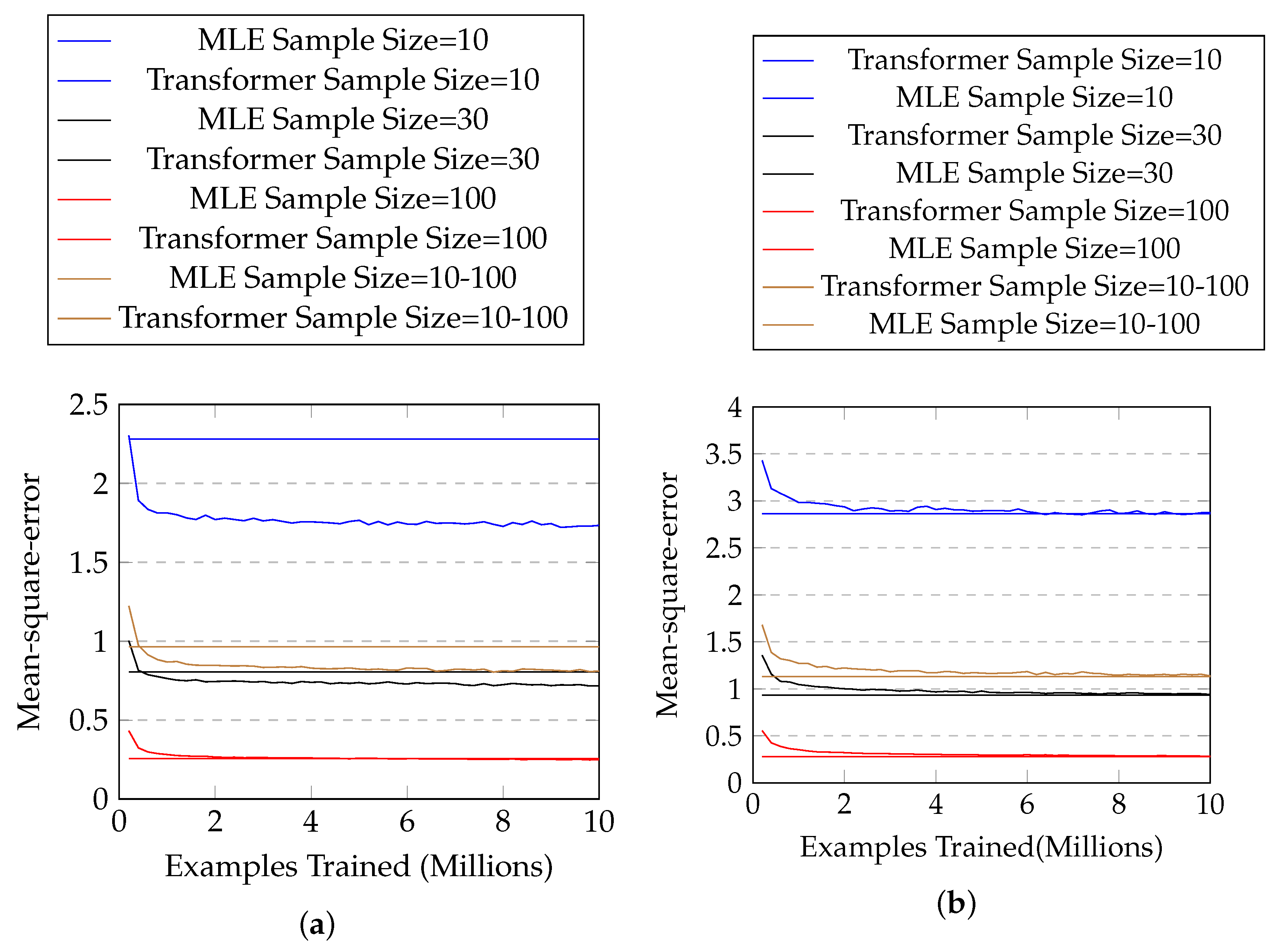
The results are shown in Figure 4a, and Table 4 shows the mean and standard deviation of the mean-square-error of the two approaches for each sample size. One can see that our approach solidly beats maximum likelihood estimation in every sample size (with p-value close to zero in two-sample t-tests), especially when the sample size is small.

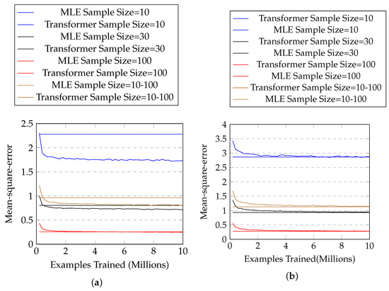
Figure 4. (a) The mean-square-error with #training examples for normal distributions with known parameter ranges. The horizontal lines represent mean-square-errors of MLE, and the curves represent those of our approach. (b) Those for normal distributions with unknown parameter ranges.

Table 4. The mean and standard deviation of the mean-square-error of MLE and our approach for each sample size for normal distribution with known parameter range, together with t-value and p-value from a two-sample t-test.

Sample Size	MLE (Mean/Std)	Our Approach (Mean/Std)	t-Value	p-Value
10	2.2809/3.3162	1.7337/2.3722	42.439	0.0001
30	0.8056/1.2578	0.7169/1.0949	16.8203	0.0001
100	0.2558/0.3960	0.2492/0.3786	3.8418	0.0001
10 to 100	0.9636/1.7916	0.8106/1.4343	21.0818	0.0001

4.3.2. Unknown Parameter Range

Suppose a sample is drawn from a normal distribution $\mathcal{N}(\mu ,{\sigma }^2)$, and the ranges of $\mathsf{\mu }$ and $\sigma$ are unknown. Like the case for exponential distribution, we first normalize each sample s into range $[0,1]$, in order to hide the parameters’ range from our model. Let $a=min\left(s\right)$ and $b=max\left(s\right)$. Each value $x_i$ is normalized by ${x_i}^{\prime }=(x_i-a)/(b-a)$.

Suppose the model’s outputs are ${\mu }^{*}$ and ${\sigma }^{*}$. To compute the loss, we first recover them into the original range: The estimate of $\mathsf{\mu }$ is $\widehat{\mu }=({\mu }^{*}·(b-a))+a$, and that of $\sigma$ is $\widehat{\sigma }={\sigma }^{*}·(b-a)$. Then we compare them with the true parameters, as follows:

$$loss=\mathrm{mean}-\mathrm{square}-\mathrm{error}([\widehat{\mu },\widehat{\sigma }],[\mu ,\sigma ])$$

(3)

The results are shown in Figure 4b and Table 5. One can see that our proposed approach has similar performance (no statistical significance) with MLE in most cases, but is not as good when sample size is 100.

Table 5. The mean-square-error of MLE and our approach for each sample size for normal distribution with unknown parameter range, together two-sample t-test results.

Sample Size	MLE (Mean/Std)	Our Approach (Mean/Std)	t-Value	p-Value
10	2.8637/4.4314	2.8768/4.4532	−0.6594	0.5096
30	0.9316/1.4520	0.9402/1.4704	−1.3160	0.1882
100	0.2780/0.4357	0.0182/0.0323	−2.7978	0.0051
10 to 100	1.1309/2.2248	1.1376/2.2967	−0.6626	0.5076

4.4. Beta Distribution

There is no closed form solution for maximum likelihood estimation for the parameters of a Beta distribution. Numerical solutions have been proposed (e.g., [2]), which are complex and there is no open-sourced implementation available. In the special case where the two parameters $\alpha$ and $\beta$ are between 0 and 1, one can use the method of moments [17] to estimate the parameters, and we compare that to our approach.

Table 6 shows our results of parameter estimation for Beta distribution, compared with Method of Moments. Even in the special case where 0 < $\alpha$, $\beta$ < 1, our approach outperforms the Method of Moments by a large margin. On the other hand, our approach can estimate parameters for Beta distributions of any parameters (results shown in Table 7).

Table 6. The mean-square-error of MLE and our approach for each sample size for Beta distribution with known parameter range (0 < $\alpha$, $\beta$ < 1), together two-sample t-test results.

Sample Size	MLE (Mean/Std)	Our Approach (Mean/Std)	t-Value	p-Value
10	0.0933/0.0665	0.0235/0.0261	97.7	0.0001
30	0.3313/0.2086	0.0123/0.0155	152.8	0.0001
100	0.2873/0.1904	0.0054/0.0081	148.3	0.0001
10 to 100	0.1756/0.1330	0.0131/0.0177	106.4	0.0001

Table 7. The mean-square-error of our approach for each sample size for Beta distribution with known parameter range (0.5 < $\alpha$, $\beta$ < 5).

Sample size	10	30	100	10 to 100
MSE	0.543	0.287	0.122	0.302

We can see that our approach is an ideal solution for distributions without readily known formula for parameter estimation. Traditionally, it often takes years of research time to derive a closed form or design an algorithm for parameter estimation of a particular type of distribution. In comparison, our approach only requires 60 h of machine time to train a model for each type of distribution.

5. Conclusions

In this paper, we propose a new method for parameter estimation, which converts a sample into a sequence of embeddings which can be consumed by a transformer model. The empirical study shows that the proposed approach outperforms maximum likelihood estimation (in terms of mean-square-error) in most scenarios, especially when the parameters’ ranges are known. In real-world applications, the parameters’ ranges are usually known, which makes our approach an ideal solution to estimate parameters.

References

- Meyer, J. Maximum Likelihood Estimation of Gaussian Parameters. Available online: http://jrmeyer.github.io/machinelearning/2017/08/18/mle.html (accessed on 4 October 2023).
- Owen, C.-E. Parameter Estimation for the Beta Distribution. Master’s Thesis, Brigham Young University, Provo, UT, USA, 2008. [Google Scholar]
- Vaswani, A.; Shazeer, N.; Parmar, N.; Uszkoreit, J.; Jones, L.; Gomez, A.N.; Polosukhin, I. Attention is All you Need. In Proceedings of the 31st Conference on Advances in Neural Information Processing Systems, Long Beach, CA, USA, 4–9 December 2017. [Google Scholar]
- Cobbe, K.; Kosaraju, V.; Bavarian, M.; Chen, M.; Jun, H.; Kaiser, L.; Schulman, J. Training Verifiers to Solve Math Word Problems. arXiv 2021, arXiv:2110.14168. [Google Scholar]
- Lu, P.; Qiu, L.; Yu, W.; Welleck, S.; Chang, K.W. A Survey of Deep Learning for Mathematical Reasoning. In Proceedings of the 61st Annual Meeting of the Association for Computational Linguistics, Association for Computer Linguistics, Toronto, ON, Canada, 9–14 July 2023; pp. 14605–14631. [Google Scholar]
- Cranmer, M.; Sanchez Gonzalez, A.; Battaglia, P.; Xu, R.; Cranmer, K.; Spergel, D.; Ho, S. Discovering Symbolic Models from Deep Learning with Inductive Biases. arXiv 2020, arXiv:2006.11287. [Google Scholar]
- Lim, B.; Zohren, S. Time Series Forecasting with Deep Learning: A Survey. arXiv 2020, arXiv:2004.13408. [Google Scholar] [CrossRef] [PubMed]
- Gnanadesikan, R.; Pinkham, R.S.; Hughes, L.P. Maximum Likelihood Estimation of the Parameters of the Beta Distribution from Smallest Order Statistics. Technometrics 1967, 9, 607–620. [Google Scholar] [CrossRef]
- Kutz, J.N. Machine learning for parameter estimation. Proc. Natl. Acad. Sci. USA 2023, 120, e2300990120. [Google Scholar] [CrossRef] [PubMed]
- Figueroa-Zúñiga, J.; Niklitschek-Soto, S.; Leiva, V.; Liu, S. Modeling heavy-tailed bounded data by the trapezoidal beta distribution with applications. Revstat-Stat. J. 2022, 20, 387–404. [Google Scholar]
- Nolan, S.-P.; Smerzi, A.; Pezzè, L. A machine learning approach to Bayesian parameter estimation. NPJ Quantum Inf. 2021, 7, 169. [Google Scholar] [CrossRef]
- George, D.; Huerta, E.-A. Deep Learning for Real-time Gravitational Wave Detection and Parameter Estimation: Results with Advanced LIGO Data. Phys. Lett. B 2018, 778, 64–70. [Google Scholar] [CrossRef]
- Kwon, H.Y.; Yoon, H.G.; Lee, C.; Chen, G.; Liu, K.; Schmid, A.K.; Won, C. Magnetic Hamiltonian parameter estimation using deep learning techniques. Condens. Matter Phys. 2020, 6, 39. [Google Scholar] [CrossRef] [PubMed]
- Ottens, T.; Barbieri, S.; Orton, M.R.; Klaassen, R.; van Laarhoven, H.W.; Crezee, H.; Gurney-Champion, O.J. Deep learning DCE-MRI parameter estimation: Application in pancreatic cancer. Med. Image Anal. 2022, 80, 102512. [Google Scholar] [CrossRef] [PubMed]
- Liu, Y.; Ott, M.; Goyal, N.; Du, J.; Joshi, M.; Chen, D.; Stoyanov, V. RoBERTa: A Robustly Optimized BERT Pretraining Approach. arXiv 2019, arXiv:1907.11692. [Google Scholar]
- Devlin, J.; Chang, M.W.; Lee, K.; Toutanova, K. BERT: Pre-training of Deep Bidirectional Transformers for Language Understanding. In Proceedings of the 2019 Conference of the North American Chapter of the Association for Computational Linguistics: Human Language Technologies, Minneapolis, MN, USA, 2–7 June 2019. [Google Scholar]
- Beta Distribution. Available online: https://www.itl.nist.gov/div898/handbook/eda/section3/eda366h.htm (accessed on 6 October 2023).
Disclaimer/Publisher’s Note: The statements, opinions and data contained in all publications are solely those of the individual author(s) and contributor(s) and not of MDPI and/or the editor(s). MDPI and/or the editor(s) disclaim responsibility for any injury to people or property resulting from any ideas, methods, instructions or products referred to in the content. |
© 2024 by the authors. Licensee MDPI, Basel, Switzerland. This article is an open access article distributed under the terms and conditions of the Creative Commons Attribution (CC BY) license (https://creativecommons.org/licenses/by/4.0/).