Randomized Nonuniform Sampling for Random Signals Bandlimited in the Special Affine Fourier Transform Domain

Abstract

The nonuniform sampling and reconstruction of bandlimited random signals in the SAFT domain is discussed in the paper, where the nonuniform samples are obtained by randomly disturbing the uniform sampling. First, we prove that the concerned nonuniform problem is equivalent to the process of uniform sampling after a prefilter in the statistic sense. Then, an approximate reconstruction method based on sinc interpolation is proposed for the randomized nonuniform sampling of SAFT-bandlimited random signals. Finally, we offer the mean square error estimate for the corresponding approximate recovery approach. The results generalize the conclusions of nonuniform sampling of bandlimited random signals in the FrFT and LCT domains to the SAFT domain.

1. Introduction

The special affine Fourier transform (SAFT) was first proposed in [1] to model optical systems. It offers a unified viewpoint of many known signal processing transforms, such as Fourier transform (FT), fractional Fourier transform (FrFT), linear canonical transform (LCT), Laplace transform (LT), and so on. It can also include some optical operations on light waves, such as rotation, magnification, hyperbolic transformation, free space propagation, Lens transformation, and so on. The SAFT is also called the offset linear canonical transform (OLCT) since it is defined by offsetting two extra parameters on the basis of the LCT [2]. It has been proven that the SAFT is a useful tool for signal processing, communications, quantum mechanics and optics [3,4,5,6]. Many classical results such as Zak transform, Poisson summation formula, uncertainty principles, and convolution theorems are established in the SAFT domain [7,8,9,10].

We let

$$A=\left[\begin{array}{ccc}a& b& u_0\\ c& d& {\omega }_0\end{array}\right]$$

(1)

be a matrix with six real parameters satisfying $ad-bc=1$. The continuous-time SAFT associated with the parameter matrix A of signal $f\left(t\right)$ is defined as in [1],

$$F_A\left(u\right)=SAFT\left[f\right]\left(u\right)=\left\{\begin{array}{c}{\int }_{-\infty }^{+\infty }f\left(t\right)K_A(t,u)dt,b\ne 0,\hfill \\ \sqrt{d}e\frac{jcd{\left(u-u_0\right)}^2}{2}+j{w}_{0}uf\left[d\left(u-u_0\right)\right],b=0,\hfill \end{array}\right.$$

(2)

where kernel function $K_A(t,u)$ is given by

$$K_A(t,u)=\sqrt{\frac{1}{2\pi jb}}{e}^{\frac{jd{u}_0^2}{2b}}{e}^{\frac{j}{2b}\left[a{t}^2+2t\left(u_0-u\right)-2u\left(d{u}_0-b{w}_0\right)+d{u}^2\right]}.$$

(3)

We only restrict our attention to the case of $b\ne 0$ because case $b=0$ is essentially a chirp multiplication. We suppose that x and k are position and wave numbers, respectively; then, it is shown in [1,7,11] that the SAFT can be understood as a general inhomogeneous lossless linear mapping in phase space as

$$\left[\begin{array}{c}{x}^{\prime }\\ k^{\prime }\end{array}\right]=\left[\begin{array}{cc}a& b\\ c& d\end{array}\right]\left[\begin{array}{c}x\\ k\end{array}\right]+\left[\begin{array}{c}{u}_0\\ {\omega }_0\end{array}\right],$$

(4)

which transforms any convex body into another convex body under any linear deformations, rotations, and translations in the phase space. Condition $ad-bc=1$ is used to guarantee that the area of the body is preserved by Transform (4). The definition in (2) is just the integral representation of the wave function transform associated with (4), which is derived by the authors in [1].

It can be verified that the inverse SAFT [12] is

$$f\left(t\right)=C{\int }_{-\infty }^{+\infty }{F}_A\left(u\right)K_{A^{-1}}(u,t)du,$$

(5)

where $C=e^{\frac{j}{2}\left(cd{u}_0^2-2ad{u}_0{w}_0+ab{w}_0^2\right)}$ and

$$A^{-1}:=\left[\begin{array}{ccc}d& -b& b{\omega }_0-d{u}_0\\ -c& a& c{u}_0-a{\omega }_0\end{array}\right].$$

(6)

If matrix

$$A=\left[\begin{array}{ccc}a& b& 0\\ c& d& 0\end{array}\right]\mathrm{or}A=\left[\begin{array}{ccc}0& 1& 0\\ -1& 0& 0\end{array}\right],$$

(7)

the SAFT reduces to LCT and FT, respectively.

Sampling and reconstruction builds a connection between the continuous signals and the discrete digital signals, which is the theoretical basis of signal and processing. Beginning with the Shannon’s sampling theorem of bandlimited signals [13], various samplings such as nonuniform sampling, average sampling, dynamic sampling, random sampling, mobile sampling, timing sampling, and multi-channel sampling have been generally studied for signals bandlimited in the FT domain [14,15,16,17]. With the appearance and developments of the more general transforms, the corresponding sampling theories are extended to the signals bandlimited in the FrFT and LCT domains [3,5,18,19,20,21,22]. In particular, the sampling problems associated with the SAFT have generated wide research interests in recent years due to its extensiveness and flexibility [6,7,9,12,23,24,25], which can include more signal models. For example, it is easy to verify that signal

$$f\left(t\right)=sinc\left(t\right){\mathrm{e}}^{-\frac{i{t}^2}{2}}{e}^{-it}$$

(8)

is bandlimited in the SAFT domain associated with matrix

$$A=\left[\begin{array}{ccc}1& 1& 1\\ 0.5& 1.5& 0\end{array}\right].$$

(9)

However, $f\left(t\right)$ is not bandlimited in the FT domain. Of course, we also must pay attention to the fact that a bandlimited signal space in the SAFT domain is not shift-invariant as

$$SAFT\left[f(t-\beta )\right]\left(u\right)=e^{\frac{j}{2b}[2b\beta (a{\omega }_0-c{u}_0)+bc\beta (2u-a\beta )]}SAFT\left[f\right](u-a\beta ),$$

(10)

which is a different situation from the bandlimited space in the FT domain.

Signals in the real world often present random characteristics, and sampling for random signals bandlimited in the FT domain has been generally studied [16,26,27,28]. In recent years, there emerged a lot of research on the sampling of random signals bandlimited in the FrFT and LCT domains [29,30,31,32,33], including uniform sampling and nonuniform sampling. Nonuniform sampling is a more realistic sampling scheme due to the limitations of data acquisition and processing ability. Various nonuniform sampling schemes such as the periodic nonuniform model, the N-order recurrent nonuniform model, the migration of a finite number of uniform samples, and the general nonuniform mode have been considered for random signals bandlimited in the LCT domain [33], respectively. In particular, a randomized nonuniform sampling method with nonuniform samples being the random perturbations of uniform grids and a class of approximate recovery approaches by using sinc interpolation functions were studied in [30] for random signals bandlimited in the LCT domain, which extends the corresponding results in the FT and FrFT domains [22,34]. For random signals bandlimited in the SAFT domain, the multichannel uniform sampling theorems were established in [35], and the deterministic nonuniform sampling and reconstruction considered in [33] were studied in [12,36]. To the best of our knowledge, the randomized nonuniform sampling for random SAFT-bandlimited signals is still not seen. In the current paper, we study a kind of randomized nonuniform sampling method for SAFT-bandlimited random signals, which is a generalization of [22,30] from the reconstruction of random signals bandlimited in the FrFt and LCT domains to that of random signals bandlimited in the SAFT domain.

The paper is organized as follows. In Section 2, we offer the definition for the power spectral density in the SAFT domain. In Section 3, we study the nonuniform sampling scheme and propose an approximate recovery approach. In Section 4, the mean square error estimate for the proposed approximate recovery method is demonstrated.

2. Power Spectral Density in the SAFT Domain

Given probability space $(\mathit{\Omega },\mathcal{F},p)$, $x\left(t\right)$ is called to be a wide stationary stochastic process if it has zero mean and the auto-correlation function

$$R_{xx}(t+\tau ,t)=E\left[x(t+\tau )x^{*}\left(t\right)\right]$$

(11)

is independent of $t\in \mathbb{R}$, i.e., $R_{xx}(t+\tau ,t)=R_{xx}\left(\tau \right)$, where $E[·]$ denotes mathematical expectation and superscript * stands for the complex conjugate. Two stochastic processes $x\left(t\right)$ and $y\left(t\right)$ are said to be jointly stationary if $x\left(t\right)$ and $y\left(t\right)$ are both stationary and their cross-correlation function

$$R_{xy}(t+\tau ,t)=E\left[x(t+\tau )y^{*}\left(t\right)\right]$$

(12)

is independent of $t\in \mathbb{R}$, i.e., $R_{xy}(t+\tau ,t)=R_{xy}\left(\tau \right)$.

The SAFT cross-correlation function, the SAFT auto-power spectral density, and the SAFT cross-power spectral density are defined as in [35]. For two random signals $x\left(t\right)$ and $y\left(t\right)$, the SAFT auto-correlation function of $x\left(t\right)$ is defined as

$$R_{xx}^A\left(\tau \right)={\displaystyle \underset{T\to +\infty }{lim}}\frac{1}{2T}{\int }_{-T}^T{R}_{xx}(t+\tau ,t)e^{j\frac{a}{b}t\tau }dt.$$

(13)

Similarly, the SAFT cross-correlation function of $x\left(t\right)$ and $y\left(t\right)$ is defined as

$$R_{xy}^A\left(\tau \right)={\displaystyle \underset{T\to +\infty }{lim}}\frac{1}{2T}{\int }_{-T}^T{R}_{xy}(t+\tau ,t)e^{j\frac{a}{b}t\tau }dt.$$

(14)

Remark 1.

If random signal $\tilde{x}\left(t\right)=x\left(t\right)e^{j\frac{a}{2b}{t}^2}$ is stationary, then $x_1\left(t\right)=\tilde{x}\left(t\right)e^{j\frac{u_0}{b}t}$ is also stationary. In fact,

$$R_{x_1{x}_1}(t+\tau ,t)=e^{\frac{j{u}_0\tau }{b}}{R}_{\tilde{x}\tilde{x}}(t+\tau ,t).$$

(15)

Moreover, one has

$$\begin{array}{cc}\hfill R_{\tilde{x}\tilde{x}}(t+\tau ,t)& =E\left[\tilde{x}(t+\tau ){\tilde{x}}^{*}\left(t\right)\right]\hfill \\ & =E\left[x(t+\tau )e^{j\frac{a}{2b}{(t+\tau )}^2}{x}^{*}\left(t\right)e^{-j\frac{a}{2b}{t}^2}\right]\hfill \\ & =E\left[x(t+\tau )x^{*}\left(t\right)e^{j\frac{a}{2b}{\tau }^2}{e}^{j\frac{at\tau }{b}}\right]\hfill \\ & =R_{xx}(t+\tau ,t)e^{j\frac{at\tau }{b}}{e}^{j\frac{a}{2b}{\tau }^2}.\hfill \end{array}$$

(16)

Therefore, $R_{xx}(t+\tau ,t)e^{\frac{jat\tau }{b}}$ must be independent of t. In such a case, we have

$$R_{xx}^A\left(\tau \right)=R_{x_1{x}_1}\left(\tau \right)e^{-j\frac{a}{2b}{\tau }^2}{e}^{-j\frac{u_0}{b}\tau }.$$

(17)

We define the SAFT auto-power spectral density of the random signal $x\left(t\right)$ by

$$P_{xx}^A\left(u\right)=\sqrt{\frac{1}{-j2\pi b}}{e}^{-j\frac{d}{2b}{u}^2}{e}^{-j\frac{d{u}_0^2}{2b}}{e}^{j\frac{u}{b}\left(d{u}_0-b{w}_0\right)}{F}_A\left\{R_{xx}^A\left(\tau \right)\right\}\left(u\right)$$

(18)

and the SAFT cross-power spectral density of the random signals $x\left(t\right)$ and $y\left(t\right)$ as

$$P_{xy}^A\left(u\right)=\sqrt{\frac{1}{-j2\pi b}}{e}^{-j\frac{d}{2b}{u}^2}{e}^{-j\frac{d{u}_0^2}{2b}}{e}^{j\frac{u}{b}\left(d{u}_0-b{w}_0\right)}{F}_A\left\{R_{xy}^A\left(\tau \right)\right\}\left(u\right).$$

(19)

It follows from (2) and (18) that

$$\begin{array}{cc}\hfill R_{xx}^A\left(\tau \right)& =C·{\int }_{-\infty }^{+\infty }{P}_{xx}^A\left(u\right)1/\sqrt{\frac{1}{-j2\pi b}}{e}^{j\frac{d}{2b}{u}^2}{e}^{j\frac{d}{2b}{u}_0^2}{e}^{-j\frac{u}{b}\left(d{u}_0-b{w}_0\right)}\sqrt{\frac{1}{-j2\pi b}}\hfill \\ \hfill & \times e^{-j\frac{a}{2b}{(b{w}_0-d{u}_0)}^2}{e}^{-j\frac{d}{2b}{u}^2}{e}^{-j\frac{u}{b}\left(b{w}_0-d{u}_0-\tau \right)}{e}^{-j\frac{u_0}{b}\tau }{e}^{-j\frac{a}{2b}{\tau }^2}du\hfill \\ \hfill & =C·{\int }_{-\infty }^{+\infty }{P}_{xx}^A\left(u\right)e^{j\frac{d}{2b}{u}_0^2}{e}^{-j\frac{a}{2b}{(b{w}_0-d{u}_0)}^2}{e}^{j\frac{u}{b}\tau }{e}^{-j\frac{u_0}{b}\tau }{e}^{-j\frac{a}{2b}{\tau }^2}du\hfill \\ \hfill & =e^{\frac{j}{2}\left(cd{u}_0^2-2ad{u}_0{w}_0+ab{w}_0^2\right)}{\int }_{-\infty }^{+\infty }{P}_{xx}^A\left(u\right)e^{j\frac{d}{2b}{u}_0^2}{e}^{-j\frac{a}{2b}{(b{w}_0-d{u}_0)}^2}{e}^{j\frac{u}{b}\tau }{e}^{-j\frac{u_0}{b}\tau }{e}^{-j\frac{a}{2b}{\tau }^2}du\hfill \\ \hfill & ={\int }_{-\infty }^{+\infty }{P}_{xx}^A\left(u\right)e^{-j\frac{a}{2b}{\tau }^2}{e}^{j\frac{1}{b}(u-u_0)\tau }du.\hfill \end{array}$$

(20)

We let $F_1\left(u\right)=F_A\left\{f_1\left(t\right)\right\}\left(u\right)$ and $F_2\left(u\right)=F_1\left(u\right)H\left(u\right)$. The multiplicative filtering in the SAFT domain which was introduced in [35] is demonstrated in Figure 1.

We define normalized convolution

$$(f\Theta g)\left(t\right)=\frac{1}{\sqrt{2\pi }}{\int }_{\mathbb{R}}f\left(x\right)g(t-x)e^{-j\frac{a}{2b}\left(t^2-x^2\right)}dx$$

(21)

for $f,g\in L^2\left(\mathbb{R}\right)$ [5]. Then, we have the following conclusion:

Proposition 1.

We let

$$H\left(u\right)=\frac{1}{\sqrt{2\pi }}{\int }_{-\infty }^{+\infty }h\left(t\right)e^{-j\frac{\left(u-u_0\right)}{b}t}dt.$$

(22)

Then, the multiplicative filter in Figure 1 is equivalent to

$$f_2\left(t\right)=\left(f_1\Theta h\right)\left(t\right).$$

(23)

Proof. 

We only need to prove

$$F_A\left\{\left(f_1\Theta h\right)\left(t\right)\right\}\left(u\right)=F_1\left(u\right)H\left(u\right).$$

(24)

It follows from the definition of the SAFT that □

$$\begin{array}{cc}& F_A\left\{\left(f_1\Theta h\right)\left(t\right)\right\}\left(u\right)\hfill \\ \hfill & ={\int }_{\mathbb{R}}\left(f_1\Theta h\right)\left(t\right)\sqrt{\frac{1}{2\pi jb}}{e}^{\frac{jd{u}_0^2}{2b}}{e}^{\frac{j}{2b}\left[a{t}^2+2t\left(u_0-u\right)-2u\left(d{u}_0-b{w}_0\right)+d{u}^2\right]}dt\hfill \\ & =\frac{1}{\sqrt{2\pi }}{\int }_{\mathbb{R}}{\int }_{\mathbb{R}}{f}_1\left(x\right)h(t-x)e^{-j\frac{a}{2b}\left(t^2-x^2\right)}\sqrt{\frac{1}{2\pi jb}}{e}^{\frac{jd{u}_0^2}{2b}}{e}^{\frac{j}{2b}\left[a{t}^2+2t\left(u_0-u\right)-2u\left(d{u}_0-b{w}_0\right)+d{u}^2\right]}dxdt\hfill \\ & ={\int }_{\mathbb{R}}{f}_1\left(x\right)\sqrt{\frac{1}{2\pi jb}}{e}^{\frac{jd{u}_0^2}{2b}}{e}^{\frac{j}{2b}\left[a{x}^2+2x\left(u_0-u\right)-2u\left(d{u}_0-b{w}_0\right)+d{u}^2\right]}dx\frac{1}{\sqrt{2\pi }}{\int }_{\mathbb{R}}h(t-x)e^{\frac{j}{b}t\left(u_0-u\right)}{e}^{-\frac{j}{2b}\left[2x\left(u_0-u\right)\right]}dt\hfill \\ & ={\int }_{\mathbb{R}}{f}_1\left(x\right)\sqrt{\frac{1}{2\pi jb}}{e}^{\frac{jd{u}_0^2}{2b}}{e}^{\frac{j}{2b}\left[a{x}^2+2x\left(u_0-u\right)-2u\left(d{u}_0-b{w}_0\right)+d{u}^2\right]}dx\frac{1}{\sqrt{2\pi }}{\int }_{\mathbb{R}}h\left(t\right)e^{-j\frac{\left(u-u_0\right)}{b}t}dt\hfill \\ & =F_1\left(u\right)H\left(u\right).\hfill \end{array}$$

(25)

Lemma 1

([35]). We suppose that $x\left(t\right)$ and $y\left(t\right)$ are the input and output random signals in Figure 1, respectively; then,

$$P_{xy}^A\left(u\right)=H\left(u\right)P_{xx}^A\left(u\right)$$

(26)

and

$$P_{yy}^A\left(u\right)={\left|H\left(u\right)\right|}^2{P}_{xx}^A\left(u\right).$$

(27)

3. Nonuniform Sampling and Approximate Recovery

The sampling and reconstruction of random signals bandlimited in the SAFT domain based on nouniform samples with random characteristics are studied in this section.

Definition 1

([35]). We say that random signal $x\left(t\right)$ is SAFT-bandlimited (or bandlimited in the SAFT domain) if its SAFT power spectral density $P_{xx}^A\left(u\right)$ satisfies

$$P_{xx}^A\left(u\right)=0,\left|u\right|>u_r,$$

(28)

where $u_r$ is called the bandwidth.

Lemma 2.

We suppose that random signal $x\left(t\right)$ is SAFT-bandlimited with bandwidth $u_r$ and $\tilde{x}\left(t\right)=x\left(t\right)e^{j\frac{a}{2b}{t}^2}$ is stationary. Then, $x_1\left(t\right)$ is FT-bandlimited with bandwidth $\frac{u_r}{b}$ and the power spectral density satisfies supp$\left\{P_{x_1{x}_1}\left(u\right)\right\}\subseteq [-\frac{u_r}{b},\frac{u_r}{b}]$.

Proof. 

Since $x_1\left(t\right)$ is stationary, it follows from (17) and (18) that

$$\begin{array}{cc}\hfill P_{xx}^A\left(u\right)& =\sqrt{\frac{1}{-j2\pi b}}{e}^{-j\frac{d}{2b}{u}^2}{e}^{-j\frac{d}{2b}{u}_0^2}{e}^{j\frac{u}{b}\left(d{u}_0-b{w}_0\right)}{F}_A\left\{R_{xx}^A\left(\tau \right)\right\}\left(u\right)\hfill \\ & =\sqrt{\frac{1}{-j2\pi b}}{e}^{-j\frac{d}{2b}{u}^2}{e}^{-j\frac{d}{2b}{u}_0^2}{e}^{j\frac{u}{b}\left(d{u}_0-b{w}_0\right)}{F}_A\left\{R_{x_1{x}_1}\left(\tau \right)e^{-j\frac{a}{2b}{\tau }^2}{e}^{-j\frac{u_0}{b}\tau }\right\}\left(u\right)\hfill \\ & =\sqrt{\frac{1}{-j2\pi b}}{e}^{-j\frac{d}{2b}(u^2+u_0^2)}{e}^{j\frac{u}{b}\left(d{u}_0-b{w}_0\right)}{\int }_{-\infty }^{+\infty }{R}_{x_1{x}_1}\left(\tau \right)e^{-j\frac{a}{2b}{\tau }^2}{e}^{-j\frac{u_0}{b}\tau }\hfill \\ & \times \sqrt{\frac{1}{2\pi jb}}{e}^{\frac{jd{u}_0^2}{2b}}{e}^{\frac{j}{2b}\left[a{\tau }^2+2\tau \left(u_0-u\right)-2u\left(d{u}_0-b{w}_0\right)+d{u}^2\right]}d\tau \hfill \\ & =\frac{1}{2\pi b}{\int }_{-\infty }^{+\infty }{R}_{x_1{x}_1}\left(\tau \right)e^{-j\frac{u}{b}\tau }d\tau \hfill \\ & =\frac{1}{2\pi b}{P}_{x_1{x}_1}\left(\frac{u}{b}\right).\hfill \end{array}$$

(29)

Note that $P_{xx}^A\left(u\right)=0,\left|u\right|>u_r.$ Then, the desired result is proven. □

First, we show that the proposed nonuniform sampling is equivalent to the process of uniform sampling after a prefilter in the statistic sense.

Theorem 1.

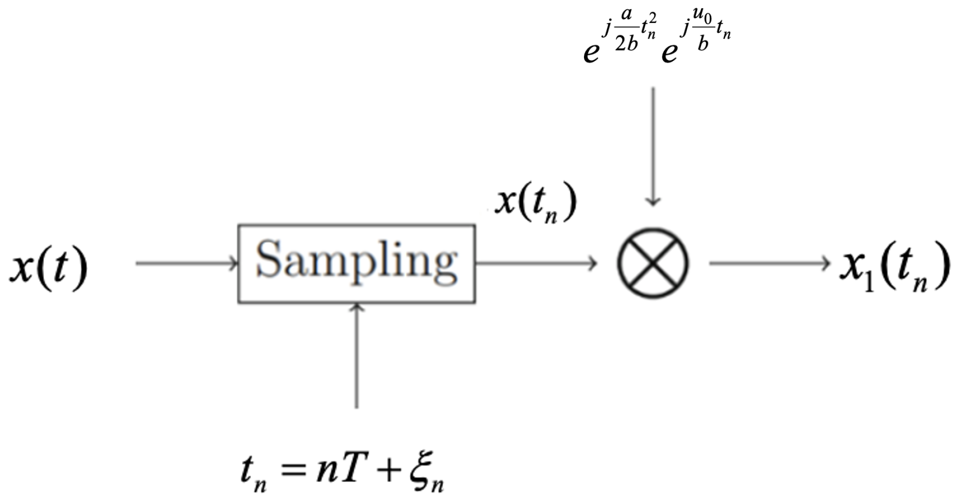
We suppose that random signal $x\left(t\right)$ is SAFT-bandlimited with bandwidth $u_r$ and $\tilde{x}\left(t\right)=x\left(t\right)e^{j\frac{a}{2b}{t}^2}$ is stationary. Then, the nonuniform sampling of $x\left(t\right)$ at sampling points $t_n=nT+{\xi }_n$ (Figure 2) is identical to the uniform sampling after SAFT filter $h_1\left(t\right)$ as in Figure 3 in the sense of second-order statistic characters, that is,

$$R_{y_1{y}_1}(nT,(n-k)T)=E\left[R_{x_1{x}_1}\left(kT+{\xi }_n-{\xi }_{n-k}\right)\right],$$

(30)

where $T\le T_N=\frac{\pi b}{u_r}$, {${\xi }_n$} is a sequence of independent identically distributed random variables with zero mean in interval $(-T/2,T/2)$. Moreover,

$$H_1\left(u\right)={\varphi }_{\xi }\left(\frac{u}{b}\right)=\frac{1}{\sqrt{2\pi }}{\int }_{-\infty }^{+\infty }{h}_1\left(t\right)e^{-j\frac{\left(u-u_0\right)}{b}t}dt,$$

(31)

and ${\varphi }_{\xi }\left(u\right)$ denotes the characteristic function of ${\xi }_n$.

Proof. 

Note that $y\left(t\right)=\left(x\Theta h_1\right)\left(t\right)$. Then, it follows from Lemma 1 that

$$P_{yy}^A\left(u\right)={\left|H_1\left(u\right)\right|}^2{P}_{xx}^A\left(u\right).$$

(32)

Moreover, one has

$$\begin{array}{cc}\hfill y_1\left(t\right)& =y\left(t\right)e^{j\frac{a}{2b}{t}^2}{e}^{j\frac{u_0}{b}t}\hfill \\ \hfill & =\frac{1}{\sqrt{2\pi }}{e}^{j\frac{u_0}{b}t}{\int }_{\mathbb{R}}x\left(s\right)h_1(t-s)e^{j\frac{a}{2b}{s}^2}ds\hfill \\ \hfill & =\frac{1}{\sqrt{2\pi }}{e}^{j\frac{u_0}{b}t}{\int }_{\mathbb{R}}\tilde{x}\left(s\right)h_1(t-s)ds.\hfill \end{array}$$

(33)

Hence, we have

$$R_{y_1{y}_1}(t+\tau ,t)=\frac{1}{2\pi }{e}^{j\frac{u_0}{b}\tau }{\int }_{\mathbb{R}}{\int }_{\mathbb{R}}{h}_1^{*}\left(s\right)R_{\tilde{x}\tilde{x}}\left(\tau -s^{\prime }+s\right)h_1\left(s^{\prime }\right)d{s}^{\prime }ds,$$

(34)

which is independent of t and $y_1\left(t\right)$ is stationary. It follows from (20) and (32) that

$$\begin{array}{cc}\hfill R_{yy}^A\left(kT\right)& ={\int }_{-u_r}^{u_r}{P}_{yy}^A\left(u\right)e^{-j\frac{a}{2b}{\left(kT\right)}^2+j\frac{1}{b}\left(u-u_0\right)kT}du\hfill \\ \hfill & ={\int }_{-u_r}^{u_r}{\left|H_1\left(u\right)\right|}^2{P}_{xx}^A\left(u\right)e^{-j\frac{a}{2b}{\left(kT\right)}^2+j\frac{1}{b}\left(u-u_0\right)kT}du.\hfill \end{array}$$

(35)

This together with (17) obtains

$$\begin{array}{cc}\hfill R_{y_1{y}_1}(nT,(n-k)T)& =R_{y_1{y}_1}\left(kT\right)\hfill \\ \hfill & =R_{yy}^A\left(kT\right)e^{j\frac{a}{2b}{\left(kT\right)}^2}{e}^{j\frac{u_0}{b}kT}\hfill \\ \hfill & =e^{j\frac{a}{2b}{\left(kT\right)}^2}{e}^{j\frac{u_0}{b}\left(kT\right)}{\int }_{-u_r}^{u_r}{\left|H_1\left(u\right)\right|}^2{P}_{xx}^A\left(u\right)e^{-j\frac{a}{2b}{\left(kT\right)}^2+j\frac{1}{b}\left(u-u_0\right)kT}du\hfill \\ \hfill & ={\int }_{-u_r}^{u_r}{\left|H_1\left(u\right)\right|}^2{P}_{xx}^A\left(u\right)e^{j\frac{u}{b}kT}du.\hfill \end{array}$$

(36)

Combining (17) and (20), we have

$$\begin{array}{cc}\hfill & E\left[R_{x_1{x}_1}\left(kT+{\xi }_n-{\xi }_{n-k}\right)\right]\hfill \\ \hfill & =E\left[R_{xx}^A\left(kT+{\xi }_n-{\xi }_{n-k}\right)e^{j\frac{a}{2b}{\left(kT+{\xi }_n-{\xi }_{n-k}\right)}^2}{e}^{j\frac{u_0}{b}\left(kT+{\xi }_n-{\xi }_{n-k}\right)}\right]\hfill \\ \hfill & =E\left[{\int }_{-u_r}^{u_r}{P}_{xx}^A\left(u\right)e^{-j\frac{a}{2b}{\left(kT+{\xi }_n-{\xi }_{n-k}\right)}^2+j\frac{1}{b}\left(u-u_0\right)\left(kT+{\xi }_n-{\xi }_{n-k}\right)}du·e^{j\frac{a}{2b}{\left(kT+{\xi }_n-{\xi }_{n-k}\right)}^2}{e}^{j\frac{u_0}{b}\left(kT+{\xi }_n-{\xi }_{n-k}\right)}\right]\hfill \\ \hfill & =E\left[{\int }_{-u_r}^{u_r}{P}_{xx}^A\left(u\right)e^{j\frac{u}{b}\left(kT+{\xi }_n-{\xi }_{n-k}\right)}du\right]\hfill \\ \hfill & ={\int }_{-u_r}^{u_r}{P}_{xx}^A\left(u\right)e^{j\frac{u}{b}kT}E\left[e^{j\frac{u}{b}\left({\xi }_n-{\xi }_{n-k}\right)}\right]du.\hfill \end{array}$$

(37)

We let $Z={\xi }_n-{\xi }_{n-k}$ and $f_Z\left(\eta \right)$ be its probability density function. We suppose that $f_{\xi }\left(\eta \right)$ is the common probability density function of ${\xi }_n$ and ${\xi }_{n-k}$, which are independent and have identical distributions; then,

$$f_Z\left(\eta \right)=\left[f_{\xi }(·)\ast f_{\xi }(-·)\right]\left(\eta \right),$$

(38)

where * denotes the convolution operator. Moreover, one has

$$\begin{array}{cc}\hfill E\left[e^{j\frac{u}{b}\left({\xi }_n-{\xi }_{n-k}\right)}\right]& ={\int }_{-\infty }^{+\infty }{f}_Z\left(\eta \right)e^{j\frac{u}{b}\eta }d\eta \hfill \\ \hfill & ={\int }_{-\infty }^{+\infty }\left[f_{\xi }(·)\ast f_{\xi }(-·)\right]\left(\eta \right)e^{j\frac{u}{b}\eta }d\eta \hfill \\ \hfill & ={\int }_{-\infty }^{+\infty }{f}_{\xi }\left(\eta \right)e^{j\frac{u}{b}\eta }d\eta ·{\int }_{-\infty }^{+\infty }{f}_{\xi }(-\eta )e^{j\frac{u}{b}\eta }d\eta \hfill \\ \hfill & ={\left|{\varphi }_{\xi }\left(\frac{u}{b}\right)\right|}^2,\hfill \end{array}$$

(39)

where

$${\varphi }_{\xi }\left(u\right)={\int }_{-\infty }^{+\infty }{f}_{\xi }\left(\eta \right)e^{ju\eta }d\eta .$$

(40)

Substituting (39) into (37) obtains

$$\begin{array}{c}\hfill E\left[R_{x_1{x}_1}\left(kT+{\xi }_n-{\xi }_{n-k}\right)\right]={\int }_{-u_r}^{u_r}{\left|{\varphi }_{\xi }\left(\frac{u}{b}\right)\right|}^2{P}_{xx}^A\left(u\right)e^{j\frac{u}{b}kT}du.\end{array}$$

(41)

This together with $H_1\left(u\right)={\varphi }_{\xi }\left(\frac{u}{b}\right)$ and (36) proves the desired result. □

In the following, we offer an approximate recovery method for bandlimited signals in the SAFT domain based on randomized nonuniform samples.

Lemma 3

([34]). We suppose that random signal $x\left(t\right)$ is bandlimited in the Fourier transform domain with bandwidth $\frac{u_r}{b}$; {${\xi }_n$} and {${\zeta }_n$} are two sequences of independent identically distributed random variables with zero mean. Then, an approximate recovery formula of nonuniform sampling for random signal $x\left(t\right)$ can be represented by

$$x^{″}\left(t\right)=\frac{T}{T_N}\sum _{n=-\infty }^{+\infty }x\left(t_n\right)h_2\left(t-{\tilde{t}}_n\right),$$

(42)

where $h_2\left(t\right)=sinc\left(\frac{u_{r}t}{b}\right)$, $sinc\left(x\right)\triangleq \frac{sinx}{x}$, $t_n=nT+{\xi }_n$, and ${\tilde{t}}_n=nT+{\zeta }_n$.

Theorem 2.

We suppose that random signal $x\left(t\right)$ is SAFT-bandlimited with bandwidth $u_r$ and $\tilde{x}\left(t\right)=x\left(t\right)e^{j\frac{a}{2b}{t}^2}$ is stationary. Then, $x\left(t\right)$ can be approximated by

$$\widehat{x}\left(t\right)=\frac{T}{T_N}{e}^{-j\frac{u_0}{b}t}{e}^{-j\frac{a}{2b}{t}^2}\sum _{n=-\infty }^{+\infty }x\left(t_n\right)e^{j\frac{a}{2b}{t}_n^2}{e}^{j\frac{u_0}{b}{t}_n}{h}_2\left(t-{\tilde{t}}_n\right),$$

(43)

where $t_n$ and ${\tilde{t}}_n$ are as in Lemma 3.

Proof. 

It follows from Lemma 2 that $x_1\left(t\right)$ is FT-bandlimited with bandwidth $\frac{u_r}{b}$. By (42), one can obtain that

$$x_1^{″}\left(t\right)=\frac{T}{T_N}\sum _{n=-\infty }^{+\infty }{x}_1\left(t_n\right)h_2\left(t-{\tilde{t}}_n\right)=\frac{T}{T_N}\sum _{n=-\infty }^{+\infty }x\left(t_n\right)e^{j\frac{a}{2b}{t}_n^2}{e}^{j\frac{u_0}{b}{t}_n}{h}_2\left(t-{\tilde{t}}_n\right)$$

(44)

is an approximation of $x_1\left(t\right)$. Note that $x\left(t\right)=e^{-j\frac{u_0}{b}t}{e}^{-j\frac{a}{2b}{t}^2}{x}_1\left(t\right)$. Then, $\widehat{x}\left(t\right)$ in (43) is an approximate recovery approach of $x\left(t\right)$ and the proof is completed. □

We let

$$\overline{x}\left(t\right)=\frac{T}{T_N}\sum _{n=-\infty }^{+\infty }{x}_1\left(t_n\right)h_2(t-{\tilde{t}}_n).$$

(45)

Figure 4 shows the approximate recovery approach based on the sinc interpolation for a SAFT-bandlimited random signal.

4. Error Estimate for Nonuniform Sampling

Since the reconstruction provided in Theorem 2 is an approximate method, we estimate the approximation error in this section.

Lemma 4.

We let $x_1\left(t\right)$ and $y_1\left(t\right)$ be the input and output random signals of the FT multiplicative filter as in Figure 5. Then,

$$P_{y_1{y}_1}\left(u\right)={\left|{\widehat{h}}_3\left(u\right)\right|}^2{P}_{x_1{x}_1}\left(u\right),$$

(46)

where ${\widehat{h}}_3\left(u\right)$ is the FT of $h_3\left(t\right)$, that is,

$${\widehat{h}}_3\left(u\right)={\int }_{\mathbb{R}}{h}_3\left(t\right)e^{-jut}dt.$$

(47)

Proof. 

Note that $y_1\left(t\right)={\int }_{-\infty }^{+\infty }{x}_1(t-u)h_3\left(u\right)du.$ Then,

$$R_{y_1{x}_1}\left(t+\tau ,t\right)=E\left[y_1(t+\tau )x_1^{*}\left(t\right)\right]={\int }_{-\infty }^{+\infty }{R}_{x_1{x}_1}\left(\tau -u\right)h_3\left(u\right)du,$$

(48)

which is independent of t. Moreover, one has

$$R_{y_1{y}_1}\left(t+\tau ,t\right)=E\left[y_1(t+\tau )y_1^{*}\left(t\right)\right]={\int }_{-\infty }^{+\infty }{R}_{y_1{x}_1}\left(\tau +u\right)h_3^{*}\left(u\right)du.$$

(49)

Taking FT on both sides of (48) and (49) obtains

$$P_{y_1{x}_1}\left(u\right)={\widehat{h}}_3\left(u\right)P_{x_1{x}_1}\left(u\right)$$

(50)

and

$$P_{y_1{y}_1}\left(u\right)={\widehat{h}}_3^{*}\left(u\right)P_{y_1{x}_1}\left(u\right).$$

(51)

Combining (50) and (51) provides

$$P_{y_1{y}_1}\left(u\right)={\left|{\widehat{h}}_3\left(u\right)\right|}^2{P}_{x_1{x}_1}\left(u\right).$$

(52)

□

Theorem 3.

We suppose that random signal $x\left(t\right)$ is SAFT-bandlimited with bandwidth $u_r$ and $\tilde{x}\left(t\right)=x\left(t\right)e^{j\frac{a}{2b}{t}^2}$ is stationary. We let $v\left(t\right)$ be an additive stationary noise with zero mean and power spectral density

$$P_{vv}\left(u\right)=T{\int }_{-u_r}^{u_r}{P}_{xx}^A\left(u_1\right)\left[1-{\left|{\varphi }_{\xi \zeta }\left(\frac{u_1}{b},-u\right)\right|}^2\right]d{u}_1,\left|u\right|\le \frac{u_r}{b},$$

(53)

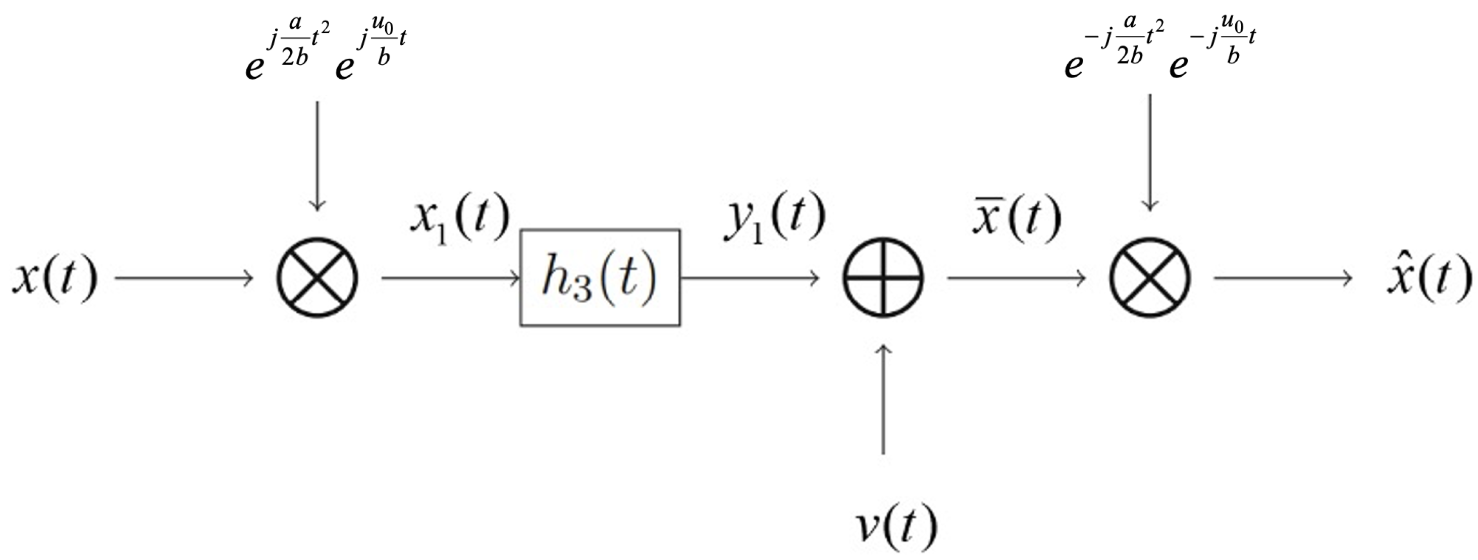
where ${\varphi }_{\xi \zeta }(s,t)$ is the joint characteristic function of random variables ${\xi }_n$ and ${\zeta }_n$. If $v\left(t\right)$ is uncorrelated with $x\left(t\right)$ and ${\varphi }_{\xi \zeta }(u,-u)$ is the frequency response of filter $h_3\left(t\right)$, then the model described in Figure 5 is identical to the procedure represented in Figure 4 in the sense of second-order statistic characters. Moreover,

$$\begin{array}{cc}\hfill E\left[{\left|\widehat{x}\left(t\right)-x\left(t\right)\right|}^2\right]& ={\int }_{-u_r}^{u_r}{P}_{xx}^A\left(u\right){\left|1-{\varphi }_{\xi \zeta }\left(\frac{u}{b},-\frac{u}{b}\right)\right|}^{2}du\hfill \\ & +\frac{T}{2\pi b}{\int }_{-u_r}^{u_r}{P}_{xx}^A\left(u\right){\int }_{-u_r}^{u_r}\left[1-{\left|{\varphi }_{\xi \zeta }\left(\frac{u}{b},-\frac{u_1}{b}\right)\right|}^2\right]d{u}_{1}du.\hfill \end{array}$$

(54)

Proof. 

It follows from Theorem 2 that

$$\overline{x}\left(t\right)=\widehat{x}\left(t\right)e^{j\frac{u_0}{b}t}{e}^{j\frac{a}{2b}{t}^2}=\frac{T}{T_N}{\displaystyle \sum _{n=-\infty }^{+\infty }}x\left(t_n\right)e^{j\frac{a}{2b}{t}_n^2}{e}^{\frac{j{u}_0{t}_n}{b}}{h}_2(t-{\tilde{t}}_n).$$

(55)

Then, one has

$$\begin{array}{cc}\hfill R_{\overline{x}\overline{x}}(t,t-\tau )& ={\left(\frac{T}{T_N}\right)}^{2}E\left[\left({\displaystyle {\displaystyle \sum _{n=-\infty }^{+\infty }}}x(nT+{\xi }_n)e^{j\frac{a}{2b}{(nT+{\xi }_n)}^2}{e}^{\frac{j{u}_0(nT+{\xi }_n)}{b}}{h}_2(t-nT-{\zeta }_n)\right)·\right.\hfill \\ & \left.\left({\displaystyle \sum _{k=-\infty }^{+\infty }}{x}^{*}(kT+{\xi }_k)e^{-j\frac{a}{2b}{(kT+{\xi }_k)}^2}{e}^{\frac{-j{u}_0(kT+{\xi }_k)}{b}}{h}_2^{*}(t-\tau -kT-{\zeta }_k)\right)\right]\hfill \\ & ={\left(\frac{T}{T_N}\right)}^2{\displaystyle \sum _{n=-\infty }^{+\infty }}{\displaystyle \sum _{k=-\infty }^{+\infty }}E\left[R_{x_1{x}_1}(nT-kT+{\xi }_n-{\xi }_k)h_2(t-nT-{\zeta }_n)h_2^{*}(t-\tau -kT-{\zeta }_k)\right].\hfill \end{array}$$

(56)

Moreover, it can be represented by two terms as

$$\begin{array}{cc}\hfill R_{\overline{x}\overline{x}}(t,t-\tau )& ={\left(\frac{T}{T_N}\right)}^2{R}_{x_1{x}_1}\left(0\right){\displaystyle \sum _{n=-\infty }^{+\infty }}E\left[h_2(t-nT-{\zeta }_n)h_2^{*}(t-\tau -nT-{\zeta }_n)\right]\hfill \\ & +{\left(\frac{T}{T_N}\right)}^2{\displaystyle \sum _{n\ne k}}E\left[R_{x_1{x}_1}(nT-kT+{\xi }_n-{\xi }_k)h_2(t-nT-{\zeta }_n)h_2^{*}(t-\tau -kT-{\zeta }_k)\right]\hfill \\ & \stackrel{\Delta }{=}I+II.\hfill \end{array}$$

(57)

Note that ${\displaystyle \sum _n}{e}^{j(u_2-u_1)nT}=2\pi {\displaystyle \sum _k}\delta \left((u_2-u_1)T-2\pi k\right)$ and

$$h_2\left(t\right)=\frac{1}{\sqrt{2\pi }}{\int }_{\mathbb{R}}{H}_2\left(u\right)e^{j\frac{u}{b}t}du=\frac{b}{\sqrt{2\pi }}{\int }_{\mathbb{R}}{H}_2\left(ub\right)e^{jut}du.$$

(58)

These together with the fact that $H_2\left(u\right)=\frac{\pi }{\sqrt{2\pi }{u}_r}{\chi }_{\left[-u_r,u_r\right]}\left(u\right)$ show that

$$\begin{array}{cc}\hfill I& =\frac{1}{2\pi }{\left(\frac{Tb}{T_N}\right)}^2{R}_{x_1{x}_1}\left(0\right){\int }_{\mathbb{R}}{\int }_{\mathbb{R}}{H}_2\left(b{u}_1\right)H_2^{*}\left(b{u}_2\right)e^{j(u_1-u_2)t}{e}^{j{u}_2\tau }{\displaystyle \sum _{n=-\infty }^{+\infty }}{e}^{j(u_2-u_1)nT}E\left[e^{j(u_2-u_1){\zeta }_n}\right]d{u}_{1}d{u}_2\hfill \\ & ={\left(\frac{Tb}{T_N}\right)}^2{R}_{x_1{x}_1}\left(0\right){\int }_{-\frac{u_r}{b}}^{\frac{u_r}{b}}\frac{1}{T}{\left|H_2\left(bu\right)\right|}^2{e}^{ju\tau }du\hfill \\ & =T{\left(\frac{b}{T_N}\right)}^2\frac{1}{2\pi }\left[{\int }_{-\frac{u_r}{b}}^{\frac{u_r}{b}}{P}_{x_1{x}_1}\left(u_1\right)d{u}_1\right]{\int }_{-\frac{u_r}{b}}^{\frac{u_r}{b}}{\left|H_2\left(bu\right)\right|}^2{e}^{ju\tau }du\hfill \\ & =\frac{T}{4{\pi }^2}{\int }_{-\frac{u_r}{b}}^{\frac{u_r}{b}}{e}^{ju\tau }\left[{\int }_{-\frac{u_r}{b}}^{\frac{u_r}{b}}{P}_{x_1{x}_1}\left(u_1\right)d{u}_1\right]du.\hfill \end{array}$$

(59)

Moreover, we have

$$\begin{array}{cc}\hfill II& ={\left(\frac{bT}{2\pi T_N}\right)}^2{\displaystyle \sum _{n\ne k}}E\left[{\int }_{-\frac{u_r}{b}}^{\frac{u_r}{b}}{P}_{x_1{x}_1}\left(u\right)e^{ju(nT-kT+{\xi }_n-{\xi }_k)}du{\int }_{\mathbb{R}}{H}_2\left(b{u}_1\right)e^{j{u}_1(t-nT-{\zeta }_n)}d{u}_1·\right.\hfill \\ & {\int }_{\mathbb{R}}{H}_2^{*}\left(b{u}_2\right)e^{-j{u}_2(t-\tau -kT-{\zeta }_k)}d{u}_2]\hfill \\ & ={\left(\frac{bT}{2\pi T_N}\right)}^2{\displaystyle \sum _{n\ne k}}{\int }_{-\frac{u_r}{b}}^{\frac{u_r}{b}}{\int }_{\mathbb{R}}{\int }_{\mathbb{R}}{P}_{x_1{x}_1}\left(u\right)H_2\left(b{u}_1\right)H_2^{*}\left(b{u}_2\right)e^{j{u}_2\tau }{e}^{j(u_1-u_2)t}{e}^{j(u-u_1)nT}{e}^{-j(u-u_2)kT}\hfill \\ & ·E\left[e^{ju{\xi }_n}{e}^{-ju{\xi }_k}{e}^{-j{u}_1{\zeta }_n}{e}^{j{u}_2{\zeta }_k}\right]d{u}_{1}d{u}_{2}du\hfill \\ & ={\left(\frac{bT}{2\pi T_N}\right)}^2{\int }_{-\frac{u_r}{b}}^{\frac{u_r}{b}}{\int }_{\mathbb{R}}{\int }_{\mathbb{R}}{P}_{x_1{x}_1}\left(u\right)H_2\left(b{u}_1\right)H_2^{*}\left(b{u}_2\right){\varphi }_{\xi \zeta }\left(u,-u_1\right){\varphi }_{\xi \zeta }^{*}\left(u,-u_2\right)e^{j{u}_2\tau }{e}^{j(u_1-u_2)t}\hfill \\ & ·\left({\displaystyle \sum _n}{e}^{j(u-u_1)nT}\right)\left({\displaystyle \sum _k}{e}^{-j(u-u_2)kT}\right)d{u}_{1}d{u}_{2}du-{\left(\frac{bT}{2\pi T_N}\right)}^2{\int }_{-\frac{u_r}{b}}^{\frac{u_r}{b}}{\int }_{\mathbb{R}}{\int }_{\mathbb{R}}{P}_{x_1{x}_1}\left(u\right)H_2\left(b{u}_1\right)H_2^{*}\left(b{u}_2\right)\hfill \\ & ·{\varphi }_{\xi \zeta }\left(u,-u_1\right){\varphi }_{\xi \zeta }^{*}\left(u,-u_2\right)e^{j{u}_2\tau }{e}^{j(u_1-u_2)t}\left({\displaystyle \sum _n}{e}^{j(u_2-u_1)nT}\right)d{u}_{1}d{u}_{2}du\hfill \\ & ={\left(\frac{b}{T_N}\right)}^2{\int }_{-\frac{u_r}{b}}^{\frac{u_r}{b}}{P_{x_1{x}_1}\left(u\right)\left|{\varphi }_{\xi \zeta }\left(u,-u\right)\right|}^2{\left|H_2\left(bu\right)\right|}^2{e}^{ju\tau }du-\hfill \\ & \frac{T}{2\pi }{\left(\frac{b}{T_N}\right)}^2{\int }_{-\frac{u_r}{b}}^{\frac{u_r}{b}}{\int }_{-\frac{u_r}{b}}^{\frac{u_r}{b}}{P}_{x_1{x}_1}\left(u_1\right){\left|{\varphi }_{\xi \zeta }\left(u_1,-u\right)\right|}^2{\left|H_2\left(bu\right)\right|}^2{e}^{ju\tau }d{u}_{1}du\hfill \\ & ={\left(\frac{b}{T_N}\right)}^2{\int }_{-\frac{u_r}{b}}^{\frac{u_r}{b}}{\left|H_2\left(bu\right)\right|}^2{e}^{ju\tau }\left[P_{x_1{x}_1}\left(u\right){\left|{\varphi }_{\xi \zeta }\left(u,-u\right)\right|}^2-\frac{T}{2\pi }{\int }_{-\frac{u_r}{b}}^{\frac{u_r}{b}}{P}_{x_1{x}_1}\left(u_1\right){\left|{\varphi }_{\xi \zeta }\left(u_1,-u\right)\right|}^{2}d{u}_1\right]\mathrm{du}\hfill \\ & =\frac{1}{2\pi }{\int }_{-\frac{u_r}{b}}^{\frac{u_r}{b}}{e}^{ju\tau }\left[P_{x_1{x}_1}\left(u\right){\left|{\varphi }_{\xi \zeta }\left(u,-u\right)\right|}^2-\frac{T}{2\pi }{\int }_{-\frac{u_r}{b}}^{\frac{u_r}{b}}{P}_{x_1{x}_1}\left(u_1\right){\left|{\varphi }_{\xi \zeta }\left(u_1,-u\right)\right|}^{2}d{u}_1\right]du.\hfill \end{array}$$

(60)

Substituting (59) and (60) into (57) obtains

$$\begin{array}{cc}\hfill R_{\overline{x}\overline{x}}(t,t-\tau )& =\frac{T}{4{\pi }^2}{\int }_{-\frac{u_r}{b}}^{\frac{u_r}{b}}\left({\int }_{-\frac{u_r}{b}}^{\frac{u_r}{b}}{P}_{x_1{x}_1}\left(u_1\right)\left[1-{\left|{\varphi }_{\xi \zeta }\left(u_1,-u\right)\right|}^2\right]d{u}_1\right)e^{ju\tau }du\hfill \\ & +\frac{1}{2\pi }{\int }_{-\frac{u_r}{b}}^{\frac{u_r}{b}}{e^{ju\tau }{P}_{x_1{x}_1}\left(u\right)\left|{\varphi }_{\xi \zeta }\left(u,-u\right)\right|}^{2}du.\hfill \end{array}$$

(61)

Similarly, we can obtain

$$R_{\overline{x}{x}_1}(t,t-\tau )=\frac{1}{2\pi }{\int }_{-\frac{u_r}{b}}^{\frac{u_r}{b}}{P}_{x_1{x}_1}\left(u\right)e^{ju\tau }{\varphi }_{\xi \zeta }(u,-u)du.$$

(62)

Therefore, we have

$$P_{\overline{x}\overline{x}}\left(u\right)=P_{x_1{x}_1}\left(u\right){\left|{\varphi }_{\xi \zeta }\left(u,-u\right)\right|}^2+\frac{T}{2\pi }{\int }_{-\frac{u_r}{b}}^{\frac{u_r}{b}}{P}_{x_1{x}_1}\left(u_1\right)\left[1-{\left|{\varphi }_{\xi \zeta }\left(u_1,-u\right)\right|}^2\right]d{u}_1$$

(63)

and

$$P_{\overline{x}{x}_1}\left(u\right)=P_{x_1{x}_1}\left(u\right){\varphi }_{\xi \zeta }(u,-u).$$

(64)

It follows from Lemma 4 that the first term of $P_{x_1{x}_1}\left(u\right){\left|{\varphi }_{\xi \zeta }\left(u,-u\right)\right|}^2$ in (63) is the FT power spectral density of $y_1\left(t\right)$ in Figure 5. Furthermore, since $\overline{x}\left(t\right)=y_1\left(t\right)+v\left(t\right)$ and $v\left(t\right)$ is uncorrelated with $x\left(t\right)$, then

$$\begin{array}{cc}\hfill R_{\overline{x}\overline{x}}(t+\tau ,t)& =E\left[\left(y_1(t+\tau )+v(t+\tau )\right){\left(y_1\left(t\right)+v\left(t\right)\right)}^{*}\right]\hfill \\ \hfill & =R_{y_1{y}_1}(t+\tau ,t)+R_{y_{1}v}(t+\tau ,t)+R_{v{y}_1}(t+\tau ,t)+R_{vv}(t+\tau ,t)\hfill \\ \hfill & =R_{y_1{y}_1}(t+\tau ,t)+R_{vv}(t+\tau ,t).\hfill \end{array}$$

(65)

Moreover, one has

$$P_{\overline{x}\overline{x}}\left(u\right)=P_{y_1{y}_1}\left(u\right)+P_{vv}\left(u\right),$$

(66)

which shows that the second term in (63) is just the power spectral density of $v\left(t\right)$, that is,

$$\begin{array}{cc}\hfill P_{vv}\left(u\right)& =\frac{T}{2\pi }{\int }_{-\frac{u_r}{b}}^{\frac{u_r}{b}}{P}_{x_1{x}_1}\left(u_1\right)\left[1-{\left|{\varphi }_{\xi \zeta }\left(u_1,-u\right)\right|}^2\right]d{u}_1\hfill \\ \hfill & =T{\int }_{-u_r}^{u_r}{P}_{xx}^A\left(u_1\right)\left[1-{\left|{\varphi }_{\xi \zeta }\left(\frac{u_1}{b},-u\right)\right|}^2\right]d{u}_1,\left|u\right|\le \frac{u_r}{b}.\hfill \end{array}$$

(67)

Therefore, the model described in Figure 5 is identical to the procedure represented in Figure 4 in the sense of second-order statistic characters.

Next, we estimate $E\left[{\left|\widehat{x}\left(t\right)-x\left(t\right)\right|}^2\right]$. Let $\epsilon \left(t\right)=\widehat{x}\left(t\right)-x\left(t\right)$. Combining (29) and (63), we obtain

$$\begin{array}{cc}\hfill P_{\widehat{x}\widehat{x}}^A\left(u\right)& =\frac{1}{2\pi b}{P}_{\overline{x}\overline{x}}\left(\frac{u}{b}\right)\hfill \\ \hfill & =\frac{1}{2\pi b}{P}_{x_1{x}_1}\left(\frac{u}{b}\right){\left|{\varphi }_{\xi \zeta }\left(\frac{u}{b},-\frac{u}{b}\right)\right|}^2+\frac{T}{4{\pi }^{2}b}{\int }_{-\frac{u_r}{b}}^{\frac{u_r}{b}}{P}_{x_1{x}_1}\left(u_1\right)\left[1-{\left|{\varphi }_{\xi \zeta }\left(u_1,-\frac{u}{b}\right)\right|}^2\right]d{u}_1\hfill \\ \hfill & =P_{xx}^A\left(u\right){\left|{\varphi }_{\xi \zeta }\left(\frac{u}{b},-\frac{u}{b}\right)\right|}^2+\frac{T}{2\pi b}{\int }_{-u_r}^{u_r}{P}_{xx}^A\left(u_1\right)\left[1-{\left|{\varphi }_{\xi \zeta }\left(\frac{u_1}{b},-\frac{u}{b}\right)\right|}^2\right]d{u}_1.\hfill \end{array}$$

(68)

Similarly, we can obtain

$$P_{\widehat{x}x}^A\left(u\right)=P_{xx}^A\left(u\right){\varphi }_{\xi \zeta }\left(\frac{u}{b},-\frac{u}{b}\right).$$

(69)

In fact, it is easy to see that

$$\begin{array}{cc}\hfill R_{\overline{x}{x}_1}\left(t+\tau ,t\right)& =E\left[\widehat{x}(t+\tau )e^{j\frac{u_0}{b}(t+\tau )}{e}^{j\frac{a}{2b}{(t+\tau )}^2}{x}^{*}\left(t\right)e^{-j\frac{u_0}{b}t}{e}^{-j\frac{a}{2b}{t}^2}\right]\hfill \\ \hfill & =R_{\widehat{x}x}\left(t+\tau ,t\right)e^{j\frac{u_0}{b}\tau }{e}^{j\frac{a}{b}t\tau }{e}^{j\frac{a}{2b}{\tau }^2}.\hfill \end{array}$$

(70)

Therefore, $R_{\widehat{x}x}\left(t+\tau ,t\right)e^{j\frac{a}{b}t\tau }$ is independent of t due to (62). Then,

$$\begin{array}{cc}\hfill R_{\widehat{x}x}^A\left(\tau \right)=& R_{\widehat{x}x}\left(t+\tau ,t\right)e^{j\frac{a}{b}t\tau }\hfill \\ \hfill =& R_{\overline{x}{x}_1}\left(t+\tau ,t\right)e^{-j\frac{u_0}{b}\tau }{e}^{-j\frac{a}{2b}{\tau }^2}.\hfill \end{array}$$

(71)

Moreover, it follows from (19) that

$$\begin{array}{cc}\hfill P_{\widehat{x}x}^A\left(u\right)& =\sqrt{\frac{1}{-j2\pi b}}{e}^{-j\frac{d}{2b}{u}^2}{e}^{-j\frac{d}{2b}{u}_0^2}{e}^{j\frac{u}{b}\left(d{u}_0-b{w}_0\right)}{F}_A\left\{R_{\overline{x}{x}_1}\left(\tau \right)e^{-j\frac{u_0}{b}\tau }{e}^{-j\frac{a}{2b}{\tau }^2}\right\}\left(u\right)\hfill \\ \hfill & =\sqrt{\frac{1}{-j2\pi b}}{e}^{-j\frac{d}{2b}(u^2+u_0^2)}{e}^{j\frac{u}{b}\left(d{u}_0-b{w}_0\right)}{\int }_{-\infty }^{+\infty }{R}_{\overline{x}{x}_1}\left(\tau \right)e^{-j\frac{u_0}{b}\tau }{e}^{-j\frac{a}{2b}{\tau }^2}\sqrt{\frac{1}{2\pi jb}}{e}^{\frac{jd{u}_0^2}{2b}}\hfill \\ \hfill & ·e^{\frac{j}{2b}\left[a{\tau }^2+2\tau \left(u_0-u\right)-2u\left(d{u}_0-b{w}_0\right)+d{u}^2\right]}d\tau \hfill \\ \hfill & =\frac{1}{2\pi b}{\int }_{-\infty }^{+\infty }{R}_{\overline{x}{x}_1}\left(\tau \right)e^{-j\frac{u}{b}\tau }d\tau \hfill \\ \hfill & =\frac{1}{2\pi b}{P}_{\overline{x}{x}_1}\left(\frac{u}{b}\right)\hfill \\ \hfill & =\frac{1}{2\pi b}{P}_{x_1{x}_1}\left(\frac{u}{b}\right){\varphi }_{\xi \zeta }\left(\frac{u}{b},-\frac{u}{b}\right)\hfill \\ \hfill & =P_{xx}^A\left(u\right){\varphi }_{\xi \zeta }\left(\frac{u}{b},-\frac{u}{b}\right).\hfill \end{array}$$

(72)

Hence, the SAFT auto-power spectral density of reconstruction error $\epsilon \left(t\right)$ is

$$\begin{array}{cc}\hfill P_{\epsilon \epsilon }^A\left(u\right)& =P_{\widehat{x}\widehat{x}}^A\left(u\right)-P_{\widehat{x}x}^A\left(u\right)-P_{x\widehat{x}}^A\left(u\right)+P_{xx}^A\left(u\right)\hfill \\ \hfill & =P_{xx}^A\left(u\right){\left|{\varphi }_{\xi \zeta }\left(\frac{u}{b},-\frac{u}{b}\right)\right|}^2+\frac{T}{2\pi b}{\int }_{-u_r}^{u_r}{P}_{xx}^A\left(u_1\right)\left[1-{\left|{\varphi }_{\xi \zeta }\left(\frac{u_1}{b},-\frac{u}{b}\right)\right|}^2\right]d{u}_1\hfill \\ \hfill & -P_{xx}^A\left(u\right){\varphi }_{\xi \zeta }\left(\frac{u}{b},-\frac{u}{b}\right)-{\left[P_{xx}^A\left(u\right){\varphi }_{\xi \zeta }\left(\frac{u}{b},-\frac{u}{b}\right)\right]}^{*}+P_{xx}^A\left(u\right)\hfill \\ & =P_{xx}^A\left(u\right){\left|1-{\varphi }_{\xi \zeta }\left(\frac{u}{b},-\frac{u}{b}\right)\right|}^2+\frac{T}{2\pi b}{\int }_{-u_r}^{u_r}{P}_{xx}^A\left(u_1\right)\left[1-{\left|{\varphi }_{\xi \zeta }\left(\frac{u_1}{b},-\frac{u}{b}\right)\right|}^2\right]d{u}_1,\hfill \end{array}$$

(73)

where we use the fact that $P_{xx}^A\left(u\right)$ is real due to (29). Note that

$${\epsilon }_1\left(t\right)=\epsilon \left(t\right)e^{j\frac{u_0}{b}t}{e}^{j\frac{a}{2b}{t}^2}=(\widehat{x}\left(t\right)-x\left(t\right))e^{j\frac{u_0}{b}t}{e}^{j\frac{a}{2b}{t}^2}=\overline{x}\left(t\right)-x_1\left(t\right).$$

(74)

Then, ${\epsilon }_1\left(t\right)$ is stationary. Moreover, it follows from (17) and (20) that

$$\begin{array}{cc}& E\left[{\left|\epsilon \left(t\right)\right|}^2\right]=R_{{\epsilon }_1{\epsilon }_1}\left(0\right)=R_{\epsilon \epsilon }^A\left(0\right)={\int }_{-u_r}^{u_r}{P}_{\epsilon \epsilon }^A\left(u\right)du=\hfill \\ & {\int }_{-u_r}^{u_r}{P}_{xx}^A\left(u\right){\left|1-{\varphi }_{\xi \zeta }\left(\frac{u}{b},-\frac{u}{b}\right)\right|}^{2}du+\frac{T}{2\pi b}{\int }_{-u_r}^{u_r}{P}_{xx}^A\left(u\right){\int }_{-u_r}^{u_r}\left[1-{\left|{\varphi }_{\xi \zeta }\left(\frac{u}{b},-\frac{u_1}{b}\right)\right|}^2\right]d{u}_{1}du.\hfill \end{array}$$

(75)

This completes the proof. □

Remark 2.

If ${\xi }_n$ and ${\zeta }_n$ are equal to zero, then the sampling considered in the paper is just the classical uniform sampling. In such a case, ${\varphi }_{\xi \zeta }(s,t)\equiv 1$. Then, we know from Theorem 3 that

$$\begin{array}{cc}\hfill E\left[|\widehat{x}{\left(t\right)-x\left(t\right)|}^2\right]& ={\int }_{-u_r}^{u_r}{P}_{xx}^A\left(u\right){\left|1-{\varphi }_{\xi \zeta }\left(\frac{u}{b},-\frac{u}{b}\right)\right|}^{2}du\hfill \\ & +\frac{T}{2\pi b}{\int }_{-u_r}^{u_r}{P}_{xx}^A\left(u\right){\int }_{-u_r}^{u_r}\left[1-{\left|{\varphi }_{\xi \zeta }\left(\frac{u}{b},-\frac{u_1}{b}\right)\right|}^2\right]d{u}_{1}du\hfill \\ & =0.\hfill \end{array}$$

(76)

We let $T=T_N=\frac{\pi b}{u_r}$. The approximation of $x\left(t\right)$ given in (43) reduces to

$$\begin{array}{c}\hfill \widehat{x}\left(t\right)=e^{-j\frac{a}{2b}{t}^2}{\displaystyle \sum _{n=-\infty }^{+\infty }}x\left(nT\right)e^{j\frac{a}{2b}{\left(nT\right)}^2}{e}^{j\frac{u_0}{b}(nT-t)}sinc\left(\frac{u_r(t-nT)}{b}\right),\end{array}$$

(77)

which is just Theorem 3 in [35].

Remark 3.

We provide a reconstruction method based on sinc interpolation for random signals bandlimited in the SAFT domain, which is theoretically similar to that for the classical bandlimited signals in the FT domain. However, the the numerical performance may show a different case, because the strong and rapid oscillations of the chirp-modulation multiplier in the SAFT background may cause instability against a minor jitter error. As we showed in (10), a bandlimited signal space in the SAFT domain is not shift-invariant, which may require an additional step to identify both the chirp and shift parameters from the data. However, although the support of the band-limitedness is changed and the bandwidth could increase, a modest amount of oversampling can make up the effects of missing the exact determination of the offset parameters to the reconstruction, because a small shift of the signal only leads to a slight disturbance to the support in the SAFT domain.

5. Conclusions

Since the six-parameter SAFT has more flexibility relative to the four-parameter LCT and can accommodate more signal models, we extend the sampling theory with samples being the randomized perturbation of the classical uniform scheme from the FrFT and LCT backgrounds to the SAFT-bandlimited random signals. We show that the proposed nonuniform model is equivalent to the uniform sampling after a pre-filter in the statistic sense. Moreover, an approximate recovery method based on the sinc functions and the corresponding error analysis in the sense of mean square convergence are given for random signals bandlimited in the SAFT domain.

References

1. Abe, S.; Sheridan, J.T. Optical operations on wave functions as the Abelian subgroups of the special affine Fourier transformation. Opt. Lett. 1994, 19, 1801–1803. [Google Scholar] [CrossRef] [PubMed]
2. Healy, J.J.; Kutay, M.A.; Ozaktas, H.M.; Sheridan, J.T. Linear Canonical Transforms: Theory and Applications; Springer Series in Optical Sciences; Springer: New York, NY, USA, 2016. [Google Scholar]
3. Liu, X.; Shi, J.; Xiang, W.; Zhang, Q.; Zhang, N. Sampling expansion for irregularly sampled signals in fractional Fourier transform domain. Digit. Signal Process. 2014, 34, 74–81. [Google Scholar] [CrossRef]
4. Sharma, K.; Joshi, S. Signal separation using linear canonical and fractional Fourier transforms. Opt. Commun. 2006, 265, 454–460. [Google Scholar] [CrossRef]
5. Zhao, H.; Wang, R.; Song, D.; Zhang, T.; Wu, D. Extrapolation of discrete bandlimited signals in linear canonical transform domain. Signal Process. 2014, 94, 212–218. [Google Scholar] [CrossRef]
6. Xu, S.; Chai, Y.; Hu, Y. Spectral analysis of sampled band-limited signals in the offset linear canonical transform domain. Circuits Syst. Signal Process. 2015, 34, 3979–3997. [Google Scholar] [CrossRef]
7. Bhandari, A.; Zayed, A.I. Shift-invariant and sampling spaces associated with the special affine Fourier transform. Appl. Comput. Harmon. Anal. 2019, 47, 30–52. [Google Scholar] [CrossRef]
8. Huo, H.; Sun, W.; Xiao, L. Uncertainty principles associated with the offset linear canonical transform. Math. Methods Appl. Sci. 2019, 42, 466–474. [Google Scholar] [CrossRef]
9. Xiang, Q.; Qin, K. Convolution, correlation, and sampling theorems for the offset linear canonical transform. Signal Image Video Process. 2014, 8, 433–442. [Google Scholar] [CrossRef]
10. Zhi, X.; Wei, D.; Zhang, W. A generalized convolution theorem for the special affine Fourier transform and its application to filtering. Optik 2016, 127, 2613–2616. [Google Scholar] [CrossRef]
11. Gao, N.; Jiang, Y. Sampling and reconstruction of multi-dimensional bandlimited signals in the special affine Fourier transform domain. Math. Meth. Appl. Sci. 2024. [Google Scholar] [CrossRef]
12. Xu, S.; Huang, L.; Chai, Y.; He, Y. Nonuniform sampling theorems for bandlimited signals in the offset linear canonical transform. Circuits Syst. Signal Process. 2018, 37, 3227–3244. [Google Scholar]
13. Shannon, C.E. Communication in the presence of noise. Proc. IRE 1949, 37, 10–12. [Google Scholar] [CrossRef]
14. Adam, K.; Scholefield, A.; Vetterli, M. Sampling and reconstruction of bandlimited signals with multi-channel time encoding. IEEE Trans. Signal Process. 2020, 69, 1105–1119. [Google Scholar] [CrossRef]
15. Aldroubi, A.; Davis, J.; Krishtal, I. Dynamic sampling: Time-space trade-off. Appl. Comput. Harmon. Anal. 2013, 34, 495–503. [Google Scholar] [CrossRef]
16. Bass, R.F.; Gröchenig, K. Random sampling of bandlimited functions. Isral J. Math. 2010, 177, 1–28. [Google Scholar] [CrossRef]
17. Gröchenig, K.; Romero, J.L.; Unnikrishnan, J.; Vetterli, M. On minimal trajectories for mobile sampling of bandlimited fields. Appl. Comput. Harmon. Anal. 2015, 39, 487–510. [Google Scholar] [CrossRef]
18. Oktem, F.; Ozaktas, H. Exact relation between continuous and discrete linear canonical transforms. IEEE Signal Process. Lett. 2009, 16, 727–730. [Google Scholar] [CrossRef]
19. Tao, R.; Li, B.; Wang, Y.; Aggrey, G. On sampling of band-limited signals associated with the linear canonical transform. IEEE Trans. Signal Process. 2008, 56, 5454–5464. [Google Scholar]
20. Wei, D.; Ran, Q.; Li, Y. Multichannel sampling and reconstruction of bandlimited signals in the linear canonical transform domain. IET Signal Process. 2011, 5, 717–727. [Google Scholar] [CrossRef]
21. Zhao, H.; Wang, R.; Song, D. Recovery of bandlimited signals in linear canonical transform domain from noisy samples. Circuits Syst. Signal Process. 2014, 33, 1997–2008. [Google Scholar] [CrossRef]
22. Xu, L.; Zhang, F.; Tao, R. Randomized nonuniform sampling and reconstruction in fractional Fourier domain. Signal Process. 2016, 120, 311–322. [Google Scholar] [CrossRef]
23. Stern, A. Sampling of compact signals in the offset linear canonical transform domains. Signal Image Video Process. 2007, 1, 359–367. [Google Scholar] [CrossRef]
24. Xiang, Q.; Qin, K.; Huang, Q. Multichannel sampling of signals band-limited in offset linear canonical transform domains. Circuits Syst. Signal Process. 2013, 32, 2385–2406. [Google Scholar] [CrossRef]
25. Xu, S.; Chai, Y.; Hu, Y.; Jiang, C.; Li, Y. Reconstruction of digital spectrum from periodic nonuniformly sampled signals in offset linear canonical transform domain. Opt. Commun. 2015, 348, 59–65. [Google Scholar] [CrossRef]
26. Boche, H.; Mönich, U.J. Approximation of wide-sense stationary stochastic processes by Shannon sampling series. IEEE Trans. Inf. Theory 2010, 56, 6459–6469. [Google Scholar] [CrossRef]
27. Gilles, F.; Sinuk, K. Average sampling of band-limited stochastic processes. Appl. Comput. Harmon. Anal. 2013, 35, 527–534. [Google Scholar]
28. Song, Z.; Sun, W.; Zhou, X.; Hou, Z. An average sampling theorem for bandlimited stochastic processes. IEEE Trans. Inf. Theory 2007, 53, 4798–4800. [Google Scholar] [CrossRef]
29. Huo, H.; Sun, W. Sampling theorems and error estimates for random signals in the linear canonical transform domain. Signal Process. 2015, 111, 31–38. [Google Scholar] [CrossRef]
30. Huo, H.; Sun, W. Nonuniform sampling for random signals bandlimited in the linear canonical transform domain. Multidimens. Syst. Signal Process. 2020, 31, 927–950. [Google Scholar] [CrossRef]
31. Tao, R.; Zhang, F.; Wang, Y. Sampling random signals in a fractional Fourier domain. Signal Process. 2011, 91, 1394–1400. [Google Scholar] [CrossRef]
32. Xu, S.; Feng, L.; Chai, Y.; He, Y. Analysis of A-stationary random signals in the linear canonical transform domain. Signal Process. 2018, 146, 126–132. [Google Scholar] [CrossRef]
33. Xu, S.; Jiang, C.; Chai, Y.; Hu, Y.; Huang, L. Nonuniform sampling theorems for random signals in the linear canonical transform domain. Int. J. Electron. 2018, 105, 1051–1062. [Google Scholar]
34. Maymon, S.; Oppenheim, A.V. Sinc interpolation of nonuniform samples. IEEE Trans. Signal Process. 2011, 59, 4745–4758. [Google Scholar] [CrossRef]
35. Xu, S.; Feng, L.; Chai, Y.; Hu, Y.; Huang, L. Sampling theorems for bandlimited random signals in the offset linear canonical transform domain. AEU Int. J. Electron. Commun. 2017, 81, 114–119. [Google Scholar] [CrossRef]
36. Bao, Y.; Zhang, Y.; Song, Y.; Li, B.; Dang, P. Nonuniform sampling theorems for random signals in the offset linear canonical transform domain. In Proceedings of the APSIPA Annual Summit and Conference, Kuala Lumpur, Malaysia, 12–15 December 2017; pp. 94–99. [Google Scholar]
Figure 1. Multiplicative filtering in the SAFT domain.
Mathematics 12 01092 g001
Figure 2. The nonuniform sampling process.
Mathematics 12 01092 g002
Figure 3. The equivalent system of the nonuniform sampling, where the filtering through filter h 1 ( t ) means that y ˜ ( t ) = 1 2 π R x ˜ ( s ) h 1 ( t s ) d s .
Mathematics 12 01092 g003
Figure 4. The approximate reconstruction of a SAFT-bandlimited random signal.
Mathematics 12 01092 g004
Figure 5. A system equivalent to Figure 4.
Mathematics 12 01092 g005
Disclaimer/Publisher’s Note: The statements, opinions and data contained in all publications are solely those of the individual author(s) and contributor(s) and not of MDPI and/or the editor(s). MDPI and/or the editor(s) disclaim responsibility for any injury to people or property resulting from any ideas, methods, instructions or products referred to in the content.