Analysis of Probability Distributions for Modelling Extreme Rainfall Events and Detecting Climate Change: Insights from Mathematical and Statistical Methods

Abstract

Exploring the realm of extreme weather events is indispensable for various engineering disciplines and plays a pivotal role in understanding climate change phenomena. In this study, we examine the ability of 10 probability distribution functions—including exponential, normal, two- and three-parameter log-normal, gamma, Gumbel, log-Gumbel, Pearson type III, log-Pearson type III, and SQRT-ET max distributions—to assess annual maximum 24 h rainfall series obtained over a long period (1972–2022) from three nearby meteorological stations. Goodness-of-fit analyses including Kolmogorov–Smirnov and chi-square tests reveal the inadequacy of exponential and normal distributions in capturing the complexity of the data sets. Subsequent frequency analysis and multi-criteria assessment enable us to discern optimal functions for various scenarios, including hydraulic engineering and sediment yield estimation. Notably, the log-Gumbel and three-parameter log-normal distributions exhibit superior performance for high return periods, while the Gumbel and three-parameter log-normal distributions excel for lower return periods. However, caution is advised regarding the overuse of log-Gumbel, due to its high sensitivity. Moreover, as our study considers the application of mathematical and statistical methods for the detection of extreme events, it also provides insights into climate change indicators, highlighting trends in the probability distribution of annual maximum 24 h rainfall. As a novelty in the field of functional analysis, the log-Gumbel distribution with a finite sample size is utilised for the assessment of extreme events, for which no previous work seems to have been conducted. These findings offer critical perspectives on extreme rainfall modelling and the impacts of climate change, enabling informed decision making for sustainable development and resilience.

1. Introduction

Due to their impact on both the population and economy, extreme weather events have become an issue of increasing interest. In particular, focus has been placed on extreme precipitation events and, more specifically, their modelling [1]. Knowledge related to such modelling is essential for the design or diagnosis of a wide range of systems and infrastructures of interest in hydraulic, hydrological, and sedimentological engineering [2], and can also be very useful in assessing the effects of climate change and determining its impact on a territory [3,4,5].

To this end, the study of distribution functions for modelling extreme hydrological events has been carried out since the 18th century. This process has been accelerated in recent decades with the advent of the digital computer, allowing for the analysis of large hydrological databases. For example, in 1960, Greenwood and Durand provided a guide to facilitate maximum likelihood estimations of the parameters of the gamma distribution [6]. A decade later, Reich used the Gumbel, log-Gumbel, and log-Pearson type III distributions to model a series of annual maximum instantaneous flood peak discharges from 26 basins in Pennsylvania [7]. In the same year, the work of Sangal and Biswas on the three-parameter log-normal distribution is noteworthy [8]. Two years later, a report by Haan and Allen compared multiple regression and principal component regression techniques on data matrices when applied to the problem of predicting water yield in Kentucky [9]. In the same decade, Carey and Haan examined the problem of evaluating and improving stochastic model parameter estimates [10]. They described a methodology for assessing the ability of a parametric runoff model to improve short-term estimates of stochastic model parameters by extending existing runoff records. Finally, we highlight two more recent articles. In the first, Lone et al. obtained an improved Gumbel type II distribution (NIGT-II) using a T-X transformation and the Gumbel type II model [11]. In the second, Reinders and Muñoz showed that the basic hydroclimatic characteristics of a basin have a significant influence on the choice of the statistical distribution representing annual maxima [12]. At present, various extreme event distribution functions are used for the implementation of models covering different fields, including health and finance, and are even of interest for travel behaviour models in the organisation of road transport [11,13,14,15]. However, one of the first known applications of these functions was the estimation of flow rates for the design of hydraulic and civil infrastructure in general [7,8,9,10].

In hydraulic, hydrological, and sedimentological engineering, the design or diagnosis of certain structures for evacuation, control, or storage of water surface runoff or sediment transport usually involves small surface drainage or small basins. In such cases, methodologies for estimating the design discharge based on series of streamflow records are not generally applicable. A widespread alternative is the use of so-called hydrometeorological methods, in which the design flow discharge is obtained through simulating the rainfall–runoff transformation processes. Therefore, the application of these methods requires characterisation of the rainfall regime in the basin or surface drainage of interest. For this design purpose, national or regional maps of rainfall intensity–duration–frequency relationships have been proposed (see, e.g., [16,17,18]), obtained from rain gauge network databases. However, climate-change-induced increases in the magnitude or frequency of multi-daily, daily, and sub-daily precipitation [19,20,21,22,23] may lead to obsolescence of these mapping guides, thus providing underestimated values if these maps have not been updated in recent years (see, e.g., [24,25,26,27]). In this context, the optimisation of methods for fitting probability distribution functions to series of annual maximum daily rainfall records provided by rain gauges located in or near the catchment under study has gained attention.

In order to improve our knowledge on the modelling of extreme precipitation using distribution functions, we carried out a study of the models provided by 10 probability distribution functions using annual maximum 24 h rainfall data obtained from three different meteorological stations located in southern Spain. A total of 10 continuous probability distribution functions were selected, adopting the criterion that they should be commonly applied to hydroclimatic variables associated with extreme events [28,29]. The distribution functions used were as follows: (i) the exponential distribution [29], (ii) the normal distribution [29], (iii) the two-parameter log-normal distribution [30], (iv) the three-parameter log-normal distribution [8,31], (v) the gamma distribution [32], (vi) the Gumbel distribution [33,34,35], (vii) the log-Gumbel distribution [36], (viii) the Pearson type III distribution [34,37], (ix) the log-Pearson type III distribution [37,38,39], and (x) the SQRT-exponential-type distribution of maximum [40,41].

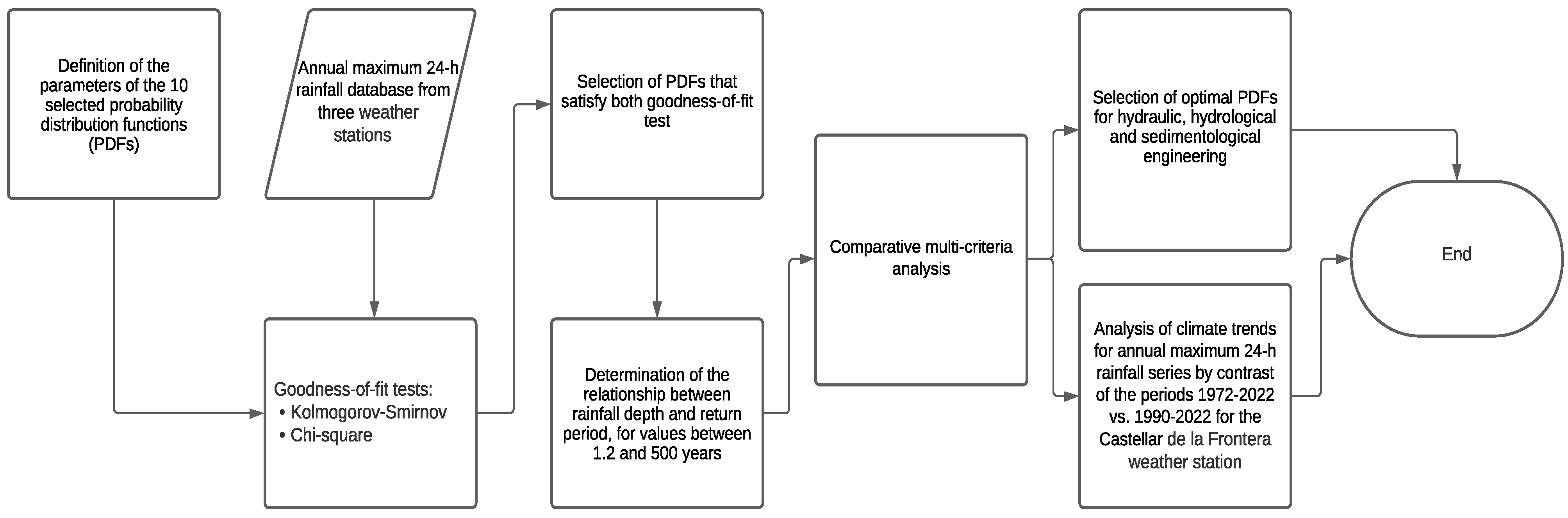
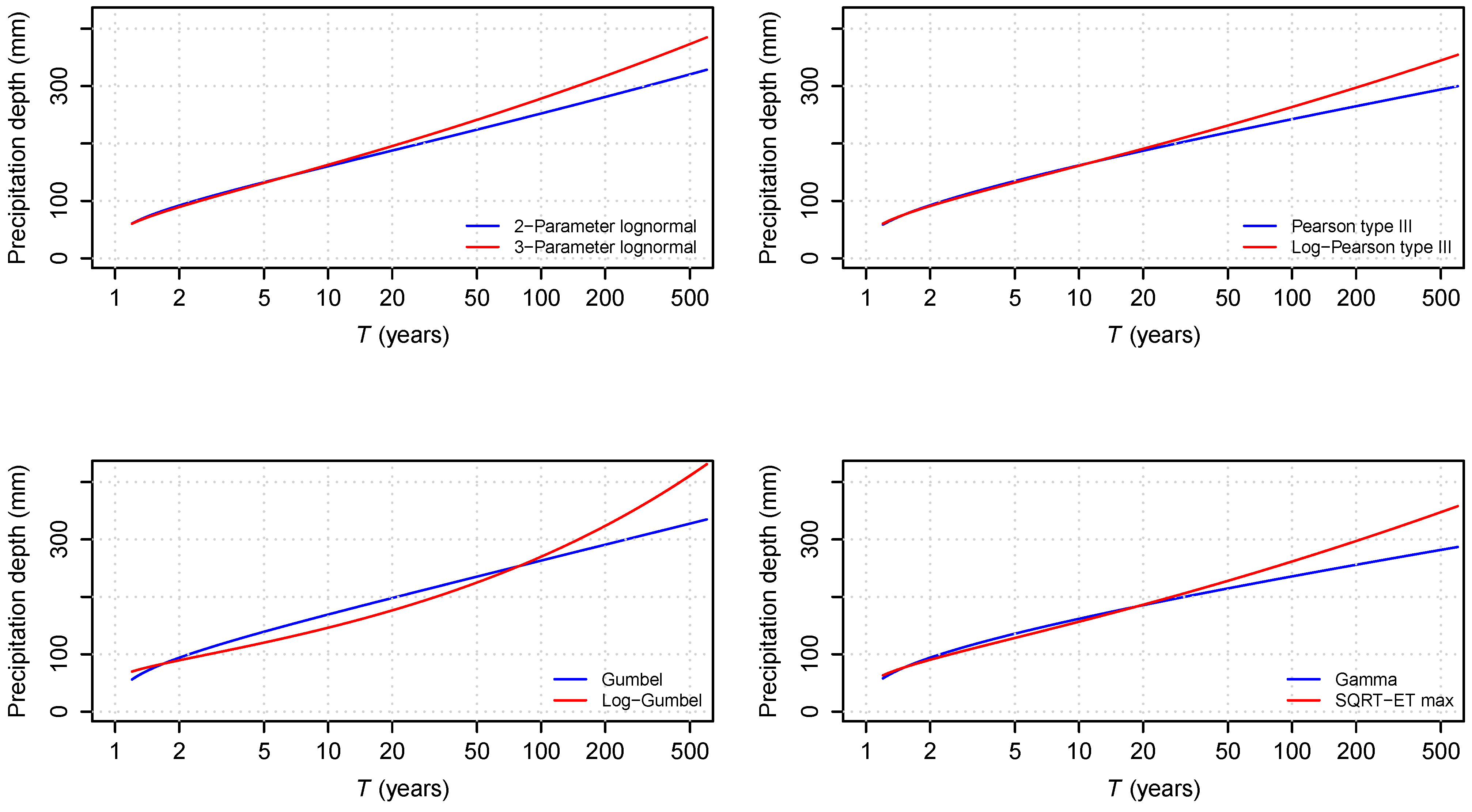
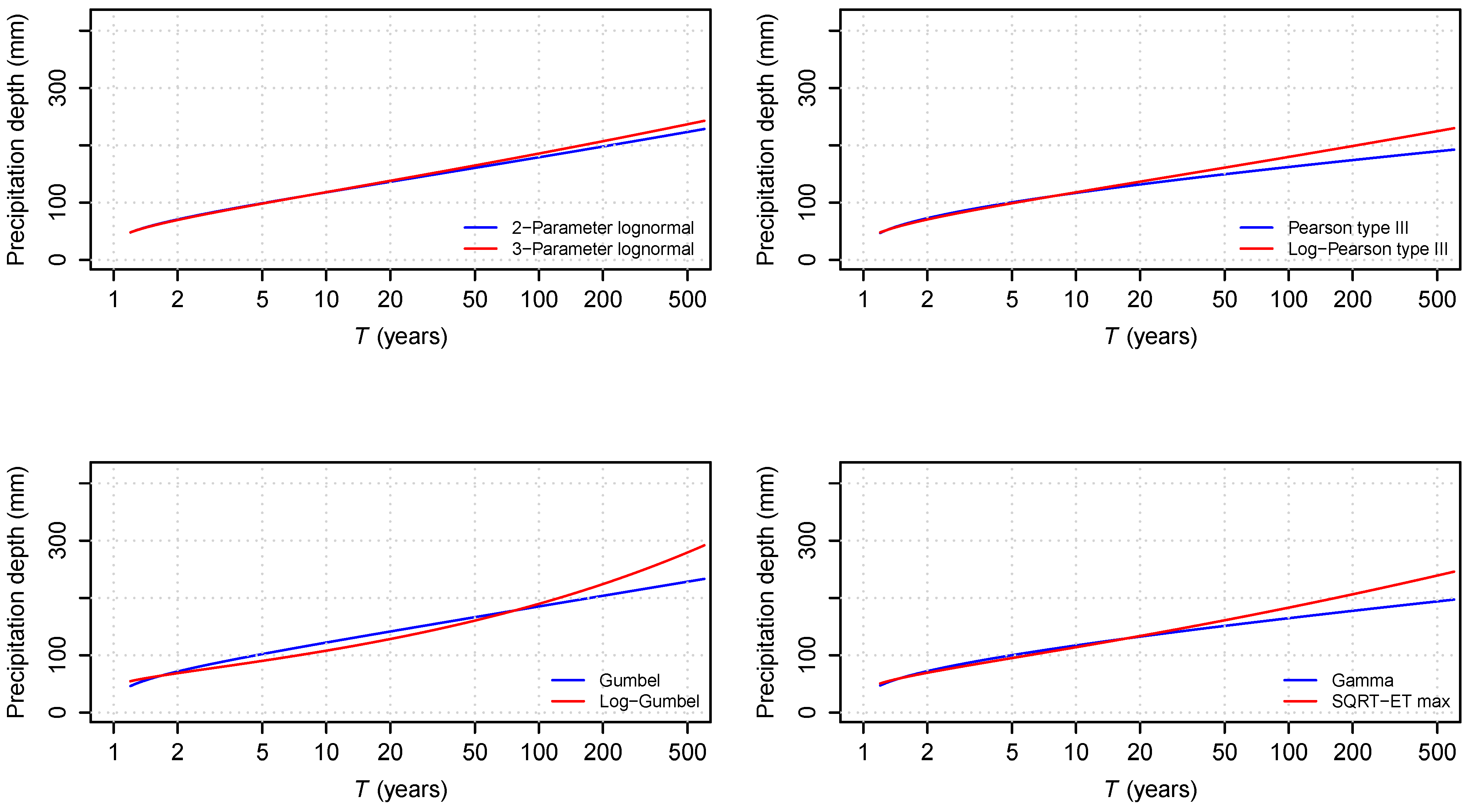
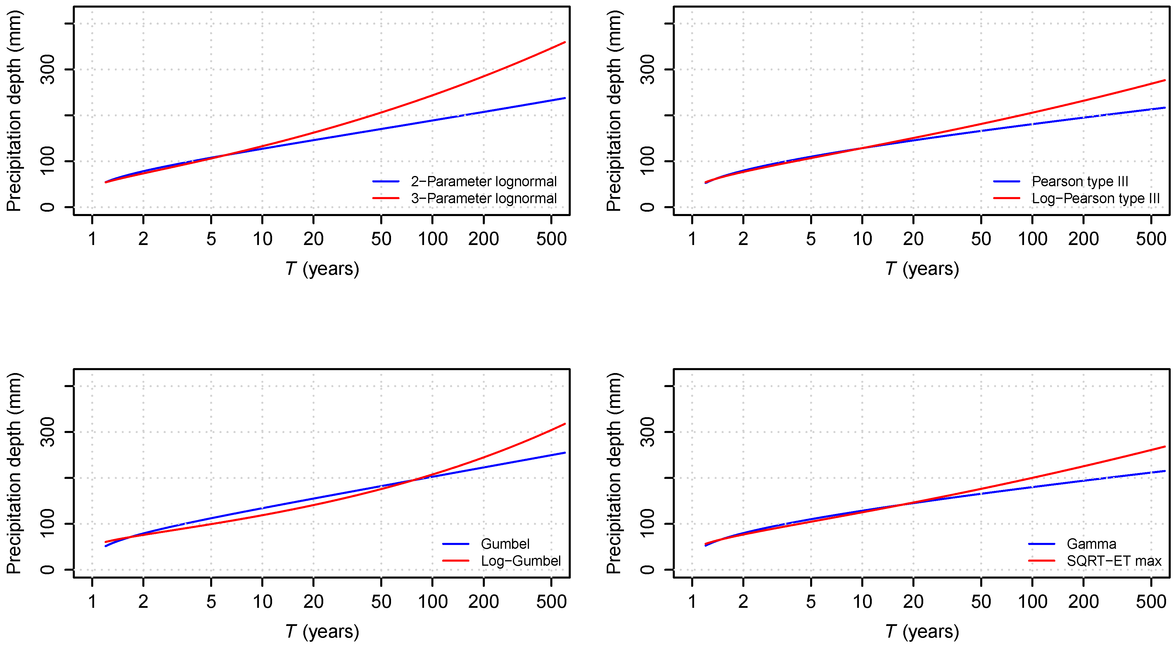
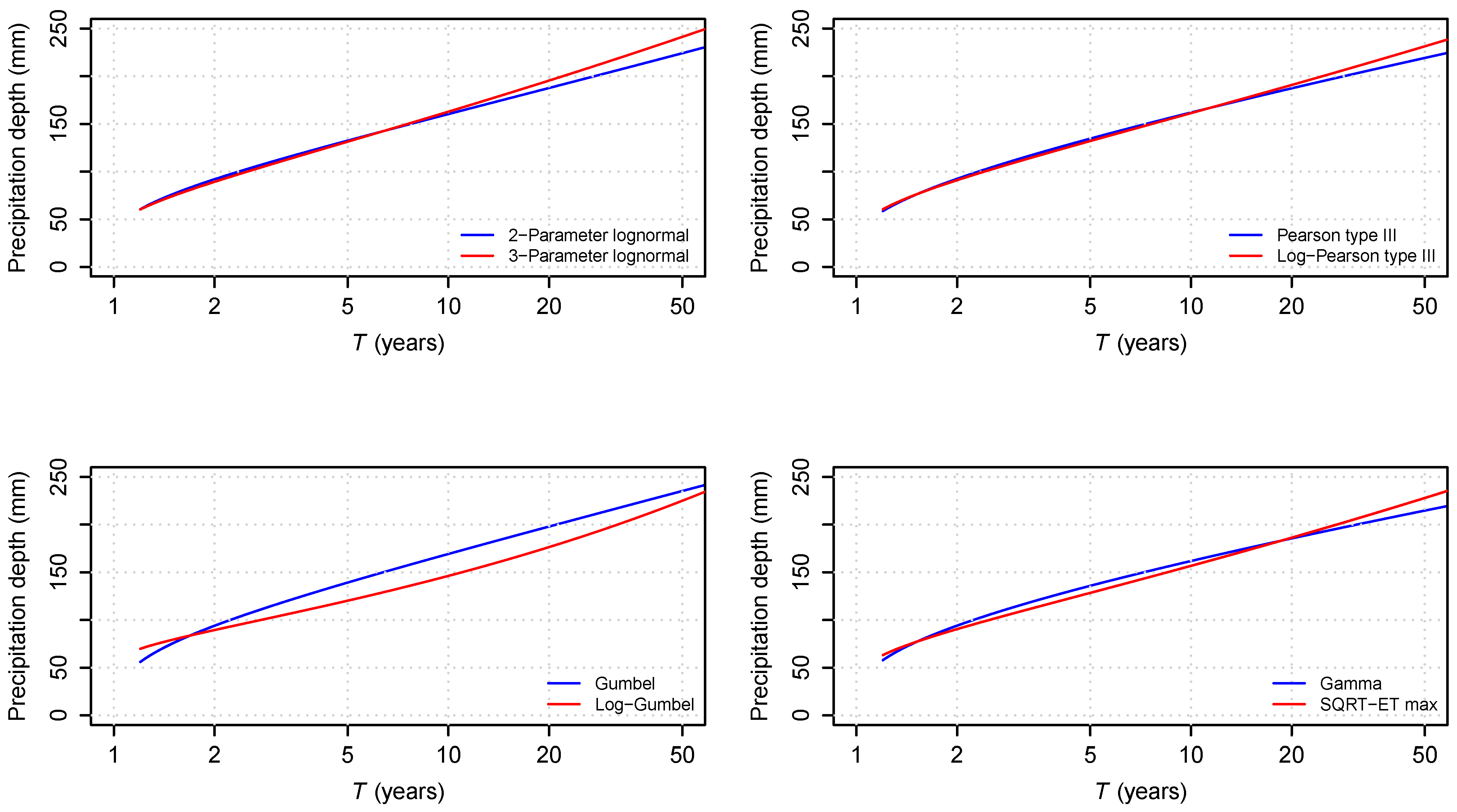
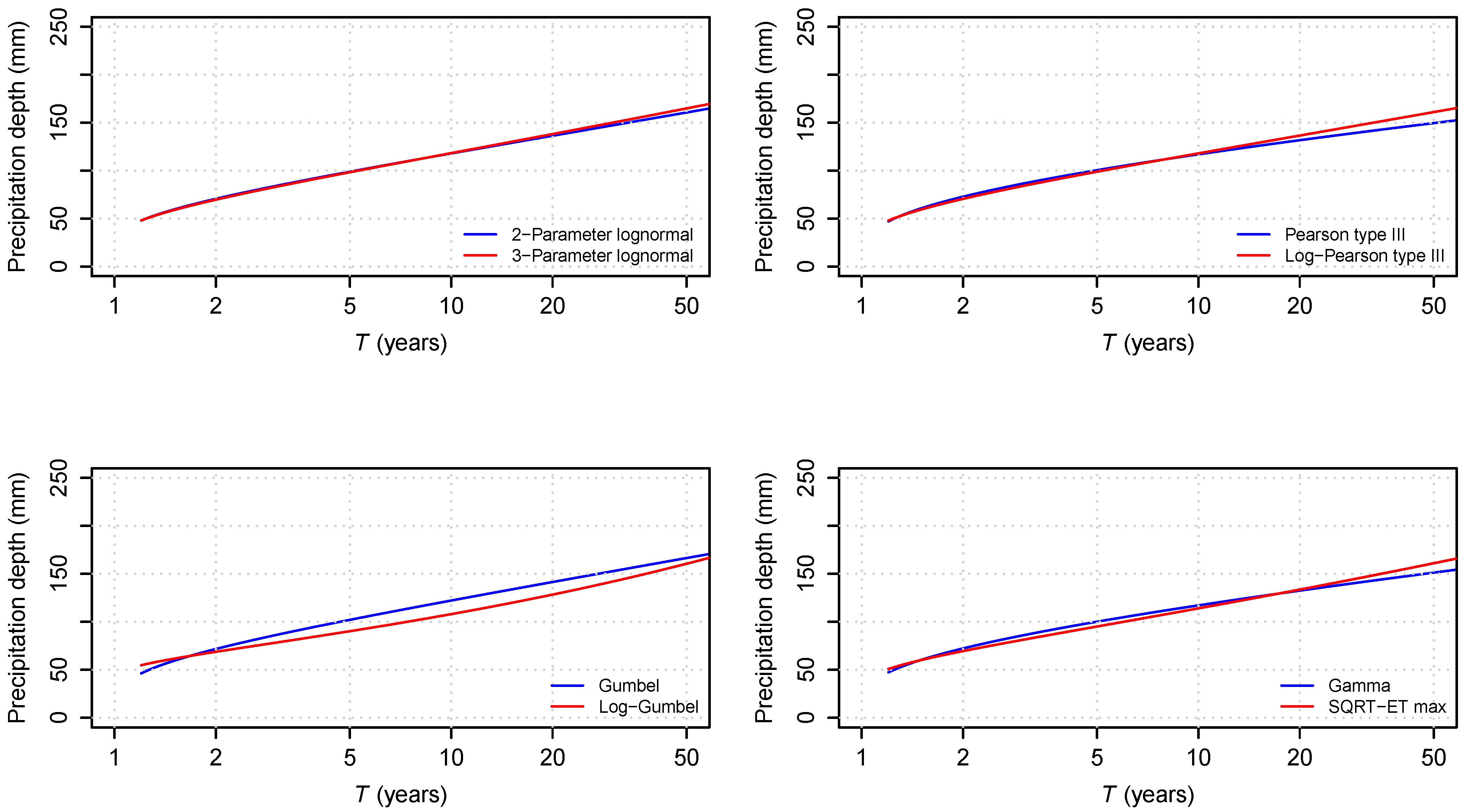
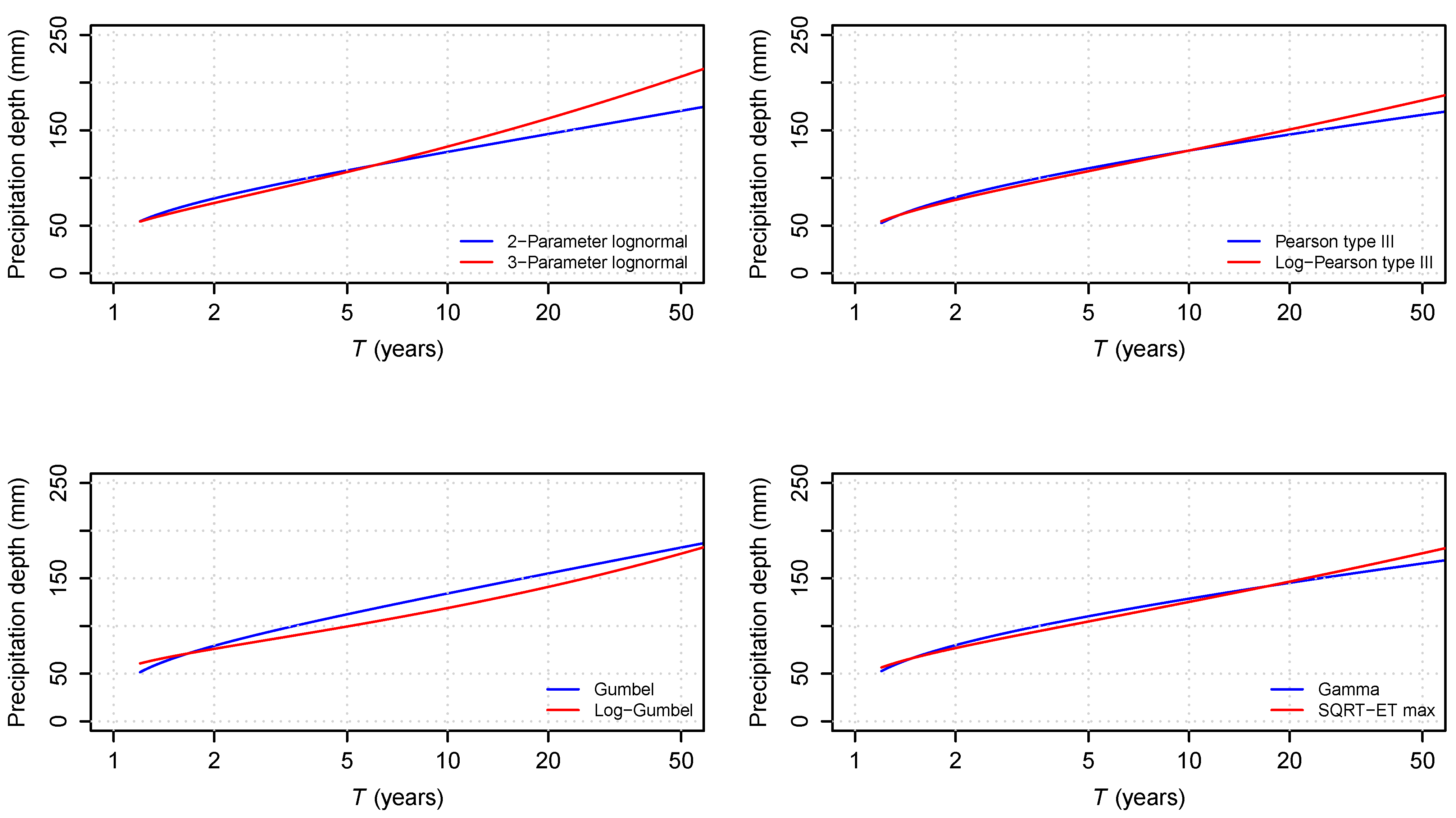
The aim of the present work is to carry out a comparative analysis of these 10 distribution functions and select those that best model the data provided by the three meteorological stations, taking into account (i) goodness-of-fit tests, (ii) the cumulative probability and return period obtained to establish design flow discharge in hydro-engineering with a conservative approach [42], and (iii) best-performance functions for return periods not exceeding 50 years suitable for estimating mean annual sediment yields. The goodness-of-fit tests used are the Kolmogorov–Smirnov test [29] and the chi-square test [43]. The return periods considered range up to 500 years, which is suitable for most engineering applications [44]. Furthermore, return periods used to estimate mean interannual sediment yields are up to 50 years, these being the most relevant periods [45]. The key innovation of this paper is as follows: a methodology for selecting rainfall probability distribution functions through the simultaneous application of two goodness-of-fit tests is established. These functions can be selected to define design storms typically applied in hydrological engineering. Although the selection can be used appropriately in many fields, their suitability for two hydrometeorological applications was taken into account in particular: (i) the design of hydraulic infrastructure favouring the conservative side criteria with high return periods of up to 500 years [44]; and (ii) the estimation of mean interannual sediment yields with designed storms for which return periods up to 50 years are most relevant [45]. Similar recent work ([46,47,48,49,50,51,52,53,54]) has considered annual maximum precipitation on hourly, daily, or monthly time scales. However, the present work aims to distinguish itself through proposing a combination of a larger number of probability distribution functions with a larger number of goodness-of-fit tests, utilised together with multiple criteria for the final choice of the most appropriate functions. The methodology, as a transversal analysis, also considers the detection of the effect of climate change through the precipitation estimates used in the two previous applications. At the same time, to the best of our knowledge, there have been no previous analyses of the Gumbel type I and log-Gumbel functions, considering a finite sample size, regarding their use in the context of the mentioned applications.

2. Materials and Methods

2.1. Methodology

The proposed methodology includes, broadly speaking, processes for the modelling of extreme rainfall using probability distribution functions, their subsequent goodness-of-fit test and, finally, a frequency analysis of the models whose fits have been accepted. The aim is to select appropriate distribution functions for hydraulic, hydrological, and sedimentological engineering, as well as to carry out a climate trend analysis. Figure 1 shows the simplified procedure (only the main operations and their organic relationships are shown).

First, we obtained annual maximum 24 h rainfall data from three weather stations located in southern Spain (Section 2.3 provides geographical information on these three weather stations and relevant information on the obtained data). From a total of 38,725 daily precipitation records provided by the State Meteorological Agency (AEMET is its acronym in Spanish) [42], 117 annual maximum records were selected. We define the probability distribution functions to be used and their parameters in Section 2.2. The distribution functions used were the (i) exponential [29], (ii) normal [29], (iii) two-parameter log-normal [30], (iv) three-parameter log-normal [8,31], (v) gamma [32], (vi) Gumbel [33,34,35], (vii) log-Gumbel [36], (viii) Pearson type III [34,37], (ix) log-Pearson type III [37,38,39], and (x) SQRT-exponential type distribution of maximum [40,41]. All calculations to fit the curves to the data sets (parameter adjustment) were performed using R software (version 4.3.2) [55]. The parameter fitting results are provided in Section 3.1.

As a preliminary visualisation of the fit of the functions to the data at each weather station, plots of cumulative probability versus precipitation depth were obtained. These plots were drawn using R software [55], and are shown in Section 3.1.

After calculating the parameters of the distribution functions, two different goodness-of-fit tests were performed: (i) Kolmogorov–Smirnov [29] and (ii) chi-square [43] tests. These tests were also carried out using R software [55]. The results of the goodness-of-fit tests are provided in Section 3.1.

With the goodness-of-fit tests performed, we proceeded to select the probability distribution functions that simultaneously satisfy both tests. It can be seen, from Section 3.1, that not all distribution functions satisfied both goodness-of-fit tests for each of the weather stations.

The relationship between precipitation depth and return period was determined using only the distribution functions that passed both goodness-of-fit tests. To be on the safe side, a return period of 500 years was set as the upper limit [44]. Section 3.2 is dedicated to the calculation of this relationship; in addition, for each of the selected functions and each of the weather stations, plots that relate the precipitation depth to the return period—also drawn using R software [55]—are provided.With the previous relationship established, a comparative multi-criteria analysis was carried out to select the most appropriate distribution functions for each case. For some types of hydraulic infrastructure, a distribution that gives a greater precipitation depth for high return period values ($T>100$ years) is preferred [56,57]. Meanwhile, in the case of the calculation of the mean interannual sediment yield, the function that provides a greater precipitation depth for low return period values ($T<50$ years) is preferred [45]. This comparative multi-criteria analysis is detailed in Section 3.2.

On the other hand, taking advantage of the fact that the data from one of the weather stations had a long time span (data from 1972), an additional comparative analysis of this data set since 1972 with the same data set since 1990 was carried out to obtain indicators of climate change. This process is discussed in Section 3.3, which also provides plots created using R software [55].

2.2. Rainfall Probability Distribution Functions

Section 2.2.1, Section 2.2.2, Section 2.2.3, Section 2.2.4, Section 2.2.5, Section 2.2.6, Section 2.2.7, Section 2.2.8, Section 2.2.9 and Section 2.2.10 present a summary of the formulation of each distribution function. Only accumulated frequency distribution functions and their parameters are explained. In order to fit distributions, parameters were estimated using one of the following methods: (i) the method of moments or (ii) the method of maximum likelihood. Some functions require numerical methods for adjustment with regional parameters. To clarify the equations, the parameters for each function are differentiated with an individual index for each case.

2.2.1. Exponential Distribution

The exponential distribution function may take any value between 0 and ∞, with a higher probability of occurrence for lower values. This function has some applications in hydrology, for example, modelling the interarrival time of droughts and other events such as a rainy day (according to a precipitation threshold value of rainfall in a day) [29].

The associated cumulative distribution function is defined in Equation (1), where the probability of obtaining a lower value than the variable x is as follows:

$$F\left(x\right)=1-e^{-\lambda x},x\ge 0,$$

(1)

where $\lambda$ is known as the rate parameter and is formulated, using the method of moments, as follows:

$$\lambda ={\displaystyle \frac{1}{\overline{x}}},$$

(2)

where $\overline{x}$ is the sample mean.

2.2.2. Normal Distribution

The normal distribution, also known as the Gaussian or bell curve, is the most common continuous distribution. In hydrology, many variables may be found to follow a normal distribution, such as temperature, relative humidity, and wind velocity. The distribution of rainfall over long periods (e.g., monthly and yearly totals) is often found to follow a normal distribution [29].

The cumulative distribution function of the normal distribution is given by:

$$F\left(x\right)={\displaystyle \frac{1}{\sqrt{2\pi {\sigma }^2}}}{\int }_{-\infty }^x{e}^{-{(t-\mu )}^2/\left(2{\sigma }^2\right)}dt,\sigma >0,$$

(3)

where $\mu$ is the mean and ${\sigma }^2$ is the variance; thus, using the method of moments, we obtain:

$$\begin{array}{cc}\hfill \mu & =\overline{x},\hfill \end{array}$$

(4)

$$\begin{array}{cc}\hfill \sigma & =S_x,\hfill \end{array}$$

(5)

where $\overline{x}$ and $S_x$ are the sample mean and sample standard deviation, respectively.

2.2.3. Two-Parameter Log-Normal Distribution

The two-parameter log-normal distribution function is a continuous probability distribution function of a random variable whose log transformation follows a normal distribution [30]; that is, if $Y=ln\left(X\right)$ follows a normal distribution, then X follows a two-parameter log-normal distribution. The two-parameter log-normal distribution is mostly applicable for variables such as the monthly precipitation depth or basin water yield, but can also be applied to extremes of variables at monthly and annual scales [29].

Its cumulative distribution function is given by:

$$F\left(x\right)={\int }_0^x{\displaystyle \frac{1}{t{\sigma }_y\sqrt{2\pi }}}{e}^{-{(ln\left(t\right)-{\mu }_y)}^2/\left(2{\sigma }_y^2\right)}dt,x\ge 0,{\sigma }_y>0,$$

(6)

where, if $Y=ln\left(X\right)$ is the logarithmic transformation, then ${\mu }_y$ (scale parameter) and ${\sigma }_y$ (shape parameter) are the mean and standard deviation of the variable Y, respectively. Hence, using the method of moments, we obtain:

$$\begin{array}{cc}\hfill {\mu }_y& =\overline{y},\hfill \end{array}$$

(7)

$$\begin{array}{cc}\hfill {\sigma }_y& =S_y,\hfill \end{array}$$

(8)

where $y=ln\left(x\right)$ is the logarithmic transformation of the sample, and $\overline{y}$ and $S_y$ are its mean and standard deviation, respectively.

2.2.4. Three-Parameter Log-Normal Distribution

The three-parameter log-normal distribution is simply the usual two-parameter log-normal distribution with a location shift; that is, if $Y=ln(X-z_0)$ follows a normal distribution, then X follows a three-parameter log-normal distribution, where $z_0$ is called the threshold parameter [31]. The distribution can be applied for frequency analysis of floods or monthly and annual water yield [8].

Its cumulative distribution function is given by:

$$F\left(x\right)={\int }_{z_0}^x{\displaystyle \frac{1}{(t-z_0){\sigma }_y\sqrt{2\pi }}}{e}^{-{(ln(t-z_0)-{\mu }_y)}^2/\left(2{\sigma }_y^2\right)}dt,{\sigma }_y>0,x\ge z_0,$$

(9)

where, if $Y=ln(X-z_0)$ is the logarithmic transformation of the shifted variable X, then ${\mu }_y$ (scale parameter) and ${\sigma }_y$ (shape parameter) are the mean and the standard deviation of the variable Y, respectively. Hence, using the method of moments, we obtain:

$$\begin{array}{cc}\hfill {\mu }_y& =\overline{y},\hfill \end{array}$$

(10)

$$\begin{array}{cc}\hfill {\sigma }_y& =S_y,\hfill \end{array}$$

(11)

where $y=ln(x-z_0)$ is the logarithmic transformation of the shifted sample, and $\overline{y}$ and $S_y$ are its mean and standard deviation, respectively. The calculation of the threshold parameter, $z_0$ (and the other two parameters, as they depend on $z_0$), requires the use of numerical methods. If N is the length of the sample, using the method of maximum likelihood, the following expression is obtained:

$$f\left(z_0\right)=\sum _{i=1}^N\left({\displaystyle \frac{1}{x_i-z_0}}({\sigma }_y^2-{\mu }_y)+{\displaystyle \frac{ln(x_i-z_0)}{x_i-z_0}}\right)=0,$$

(12)

where $x_i$, $i=1,\cdots ,N$ is the i-th element of the ordered sample and f is a function defined for the following purpose. The numerical method used to find an approximate solution to the above expression is the secant method, which is:

$$z_{n+1}=z_n-{\displaystyle \frac{z_n-z_{n-1}}{f\left(z_n\right)-f\left(z_{n-1}\right)}}f\left(z_n\right),n\ge 2.$$

(13)

The desired approximations are obtained by combining this iterative method with Equations (10)–(12). Note that the secant method requires two initial approximations for $z_0$. In this paper, we set $z_1=x_1-1$ and $z_2=z_1-10$. Furthermore, the maximum permissible error is ${10}^{-5}$; that is, we calculated the $z_0$ which verifies that $|f\left(z_0\right)|<{10}^{-5}\approx 0$.

2.2.5. Gamma Distribution

The Gamma distribution function is a continuous probability distribution function that is positively skewed on the positive side of the real line [29,32]. If X follows a gamma distribution, then X takes non-negative values only. It is very useful for the description of non-negative and asymmetric hydrological variables without the use of the logarithmic transformation. For example, it has been applied for the description of storm precipitation events [34].

The cumulative distribution function of the gamma distribution is:

$$F\left(x\right)={\displaystyle \frac{1}{{\beta }^{\alpha }\Gamma \left(\alpha \right)}}{\int }_0^x{t}^{\alpha -1}{e}^{-t/\beta }dt,x\ge 0,\alpha >0,\beta >0,$$

(14)

where $\alpha$ and $\beta$ are the shape and scale parameters, respectively, and $\Gamma \left(\alpha \right)$ is the value of the gamma function, defined as follows:

$$\Gamma \left(\alpha \right)={\int }_0^{\infty }{x}^{\alpha -1}{e}^{-x}dx.$$

(15)

If $\alpha$ is a positive integer, the gamma distribution can be treated as the sum of exponentially distributed random variables, each with the same parameter. The parameter $\alpha$ is the number of random variables following an exponential distribution and $1/\beta$ is the parameter of the exponential distributions. For this reason, the exponential distribution is a particular case of the gamma distribution, where $\alpha =1$ and $1/\beta$ is the parameter of the exponential distribution [29].

To fit the distribution, we apply the method of moments, and thus obtain:

$$\begin{array}{c}\hfill \alpha ={\displaystyle \frac{{\overline{x}}^2}{S_x^2}},\end{array}$$

(16)

$$\begin{array}{c}\hfill \beta ={\displaystyle \frac{S_x^2}{\overline{x}}},\end{array}$$

(17)

where $\overline{x}$ and $S_x$ are the sample mean and standard deviation, respectively.

2.2.6. Gumbel Distribution

The Gumbel distribution is also called the extreme value distribution type I, which was first defined by Gumbel [33,34,35]. The Gumbel distribution function is used to study variables such as the monthly and annual maximum values of 24 h rainfall or basin water yield [29]. It is also used for the frequency analysis of flood peak discharge.

Its cumulative distribution function is:

$$F\left(x\right)=e^{\pm e^{\frac{\pm (x-\beta )}{\alpha }}},-\infty <x<\infty ,\alpha >0,-\infty <\beta <\infty ,$$

(18)

where $\alpha$ and $\beta$ are the scale and location parameters, respectively; the minus sign implies the maximum value, and the plus sign implies the minimum value. In this paper, we are only interested in the maximum value, so we only use the minus sign.

According to Gumbel [33,35], fitting the distribution presents an additional difficulty, in that the following set of values has to be calculated:

$$y_i=-ln\left(ln\left({\displaystyle \frac{1+N}{i}}\right)\right),i=1,\cdots ,N,$$

(19)

where N is the sample length and i is the position of the data in the series between 1 and N. Parameters in their general form for the Gumbel distribution are as follows:

$$\begin{array}{cc}\hfill \alpha & ={\displaystyle \frac{S_x}{{\sigma }_y}},\hfill \end{array}$$

(20)

$$\begin{array}{cc}\hfill \beta =& \overline{x}-{\displaystyle \frac{{\mu }_y}{\alpha }},\hfill \end{array}$$

(21)

where $\overline{x}$ and $S_x$ are the sample mean and standard deviation, respectively, and ${\mu }_y$ and ${\sigma }_y$ are the mean and standard deviation of the set of values defined in Equation (19).

2.2.7. Log-Gumbel Distribution

The Log-Gumbel distribution is a continuous probability distribution of a random variable, defined such that its logarithmic transformation follows a Gumbel distribution; that is, if $Y=ln\left(X\right)$ follows a Gumbel distribution, then X follows a log-Gumbel distribution. It is a particular case of the Frèchet function (extreme value distribution type II) with a position parameter equal to zero [36]. As a novelty in the field of functional analysis, the log-Gumbel distribution with finite sample size has not yet been utilised in the field of extreme events. The log-Gumbel distribution (with infinite sample size) is commonly used in rainfall analysis, as precipitation data tend to fit this distribution better after a logarithmic transformation. This is particularly useful for analysing extreme rainfall events, such as high or very low rainfall.

The log-Gumbel cumulative distribution function is:

$$F\left(x\right)=e^{\pm e^{\frac{\pm (ln(x)-\beta )}{\alpha }}},x>0,\alpha >0,-\infty <\beta <\infty ,$$

(22)

where $\alpha$ and $\beta$ are the scale and location parameters, respectively; the minus sign implies the maximum value, and the plus sign implies the minimum value. We are only interested in the maximum value, so the plus sign will not be used.

To fit the curve, using the method of moments, we obtain the following equations:

$$\begin{array}{cc}\hfill \overline{x}=& {\displaystyle \frac{S_x\Gamma (1-\alpha )}{\sqrt{\Gamma (1-2\alpha )-{\Gamma }^2(1-\alpha )}}},\hfill \end{array}$$

(23)

$$\begin{array}{cc}\hfill & \beta =\ln \left({\displaystyle \frac{\overline{x}}{\Gamma (1-\alpha )}}\right),\hfill \end{array}$$

(24)

where $\overline{x}$ and $S_x$ are the sample mean and standard deviation, respectively, and $\Gamma$ is the gamma function defined in Equation (15). Equation (23) can be solved using a numerical method (e.g., the Newton–Raphson method) to obtain an estimate of the scale parameter $\alpha$. An estimate of the location parameter $\beta$ is then obtained using Equation (24).

2.2.8. Pearson Type III Distribution

The Pearson type III distribution is also called the three-parameter gamma distribution, as it is simply the usual two-parameter gamma distribution with a location shift [34,37]. The annual maximum flood peak discharge is generally described using a Pearson type III distribution [29].

Its cumulative distribution function is:

$$F\left(x\right)={\displaystyle \frac{1}{{\beta }^{\alpha }\Gamma \left(\alpha \right)}}{\int }_{x_0}^x{(t-x_0)}^{\alpha -1}{e}^{-(t-x_0)/\beta }dt,x\ge x_0,\alpha >0,\beta >0,$$

(25)

where $\alpha$, $\beta$, and $x_0$ are the shape, rate, and threshold parameters, respectively, and $\Gamma \left(\alpha \right)$ is the value of the gamma function defined in Equation (15). Applying the method of moments, the following is obtained:

$$\begin{array}{cc}\hfill & \alpha ={\displaystyle \frac{4}{C_s^2\left(x\right)}},\hfill \end{array}$$

(26)

$$\begin{array}{cc}\hfill \beta & ={\displaystyle \frac{C_s\left(x\right)S_x}{2}},\hfill \end{array}$$

(27)

$$\begin{array}{cc}\hfill x_0& =\overline{x}-{\displaystyle \frac{2S_x}{C_s\left(x\right)}},\hfill \end{array}$$

(28)

where $\overline{x}$, $S_x$, and $C_s\left(x\right)$ are the sample mean, standard deviation, and skewness coefficient, respectively.

2.2.9. Log-Pearson Type III Distribution

The log-Pearson type III distribution is a continuous probability distribution of a random variable with the logarithmic transformation that follows a Pearson type III distribution; that is, if $Y=ln\left(X\right)$ follows a Pearson type III distribution, then X follows a log-Pearson type III distribution [37,38,39]. Similarly to the Pearson III distribution, it is used in hydrology for frequency analysis. If the observations present a very high positive skew, then the log-Pearson type III distribution is suitable for modelling. This logarithmic transformation reduces the skewness, and can even transform positively skewed data into negatively skewed data [29].

The log-Pearson type III cumulative distribution function is:

$$F\left(x\right)={\displaystyle \frac{1}{{\beta }^{\alpha }\Gamma \left(\alpha \right)}}{\int }_{e^{x_0}}^x{\displaystyle \frac{{(ln\left(t\right)-x_0)}^{\alpha -1}{e}^{-(ln\left(t\right)-x_0)/\beta }}{t}}dt,x\ge e^{x_0},\alpha >0,\beta >0,$$

(29)

where $\alpha$, $\beta$, and $x_0$ are the shape, rate, and threshold parameters, respectively, and $\Gamma \left(\alpha \right)$ is the value of the gamma function defined in Equation (15). Changing the variable $(ln\left(t\right)-x_0)/\beta =u$ and putting $y=(ln\left(x\right)-x_0)/\beta$, we get

$$F\left(y\right)={\displaystyle \frac{1}{\Gamma \left(\alpha \right)}}{\int }_0^y{u}^{\alpha -1}{e}^{-u}du,y\ge 0,\alpha >0,\beta >0,$$

(30)

which is a simplified form of Equation (29). The method of moments is used to fit the distribution to the curve, thus obtaining the parametric estimate. If $z=ln\left(x\right)$ is the logarithmic transformation of the sample, then

$$\begin{array}{cc}\hfill & \alpha ={\displaystyle \frac{4}{C_s^2\left(z\right)}},\hfill \end{array}$$

(31)

$$\begin{array}{cc}\hfill \beta & ={\displaystyle \frac{C_s\left(z\right)S_z}{2}},\hfill \end{array}$$

(32)

$$\begin{array}{cc}\hfill x_0& =\overline{z}-{\displaystyle \frac{2S_z}{C_s\left(z\right)}},\hfill \end{array}$$

(33)

where $\overline{z}$, $S_z$, and $C_s\left(z\right)$ are the mean, standard deviation, and skewness coefficient of the log transformation of the sample, respectively.

2.2.10. SQRT-Exponential-Type Distribution of the Maximum (SQRT-ET Max)

This distribution was first used in Japan to model extreme rainfall, and is commonly used in the field of hydrological engineering in Spain. Its cumulative distribution function, according to Etoh and Murota [40], is as follows:

$$F\left(x\right)=e^{-k(1+\sqrt{\alpha x})e^{-\sqrt{\alpha x}}},x\ge 0,k>0,\alpha >0,$$

(34)

where k and $\alpha$ are the frequency and scale parameters, respectively. To fit the curve, the Ferrer method [41] is used, which is defined as follows:

$$\begin{array}{cc}\hfill ln\left(k\right)& =\sum _{i=0}^6{a}_{i}ln\left(C_v^i\right),\hfill \end{array}$$

(35)

$$\begin{array}{cc}\hfill ln\left(I_1\right)& =\sum _{i=0}^6{b}_i{(ln\left(k\right))}^i,\hfill \end{array}$$

(36)

$$\begin{array}{cc}\hfill \alpha & ={\displaystyle \frac{I_{1}k}{2\overline{x}(1-e^{-k})}},\hfill \end{array}$$

(37)

where $\overline{x}$ and $C_v$ are the sample mean and sample coefficient of variation, and $a_i$ and $b_i$ are tabulated parameters used to adjust the dependence relationships with $C_v$.

2.3. Rainfall Data Sets

Data are available from three weather stations located in Andalusia (southern Spain), specifically located in the province of Cadiz. The annual maximum 24 h rainfall data were obtained from these stations. The first station is Castellar de la Frontera, with data from 1972 to 2022, the second is the Almodovar reservoir station, with data from 1990 to 2022, and the third is Jimena de la Frontera, with data from 1990 to 2022.

Table 1. Geographical coordinates of the three weather stations.

Weather Station	Latitude *	Longitude *	Elevation (m asl)	Interval (Years)	Number of Data
Castellar de la Frontera	36º17′18″	−5º25′02″	45	1972–2022	51
Almodovar reservoir	36º09′15″	−5º39′03″	105	1990–2022	33
Jimena de la Frontera	36°26′18″	−5°27′16″	203	1990–2022	33

* Coordinate system: ETSR89/UTM zone 30N.

indicates the geographical locations of these three weather stations. Although the Castellar de la Frontera weather station provides data from 1972, we initially only use data from 1990 for comparison of the three weather stations with each other. Later on, all available data from this weather station are used.

Table 2. Statistical variables of the annual maximum 24 h rainfall data sets.

Statistical Variable∖Weather Station	Castellar de la Frontera	Almodóvar Reservoir	Jimena de la Frontera
Sample size	33	33	33
Annual mean rainfall (mm)	100.83	76.30	84.24
Standard Deviation (mm)	45.55	30.55	33.24
Coefficient of Variation	0.45	0.40	0.39
Coefficient of Skewness	1.13	0.68	0.83

presents a statistical summary of the 1990–2022 data sets.

3. Results and Discussion

3.1. Definitions and Goodness-of-Fit of Probability Distribution Functions

Applying Equations (1)–(37) to the recorded annual maximum 24 h rainfall series for the period of 1990–2022, the equations for the three case studies were obtained.

Table 3. Adjusted parameter values.

Distribution∖Weather Station	Castellar de la Frontera	Almodóvar Reservoir	Jimena de la Frontera
Exponential	$\lambda =0.00992$	$\lambda =0.01310$	$\lambda =0.01187$
Normal	$\mu =100.83330$	$\mu =76.30000$	$\mu =84.23939$
	$\sigma =45.54813$	$\sigma =30.54912$	$\sigma =33.23942$
Two-parameter log-normal	${\mu }_y=4.52146$	${\mu }_y=4.25790$	${\mu }_y=4.36285$
	${\sigma }_y=0.43368$	${\sigma }_y=0.39976$	${\sigma }_y=0.37760$
Three-parameter log-normal	${\mu }_y=4.22574$	${\mu }_y=4.09640$	${\mu }_y=3.65457$
	${\sigma }_y=0.56942$	${\sigma }_y=0.46174$	${\sigma }_y=0.72495$
	$z_0=20.89191$	$z_0=9.62717$	$z_0=35.04865$
Gamma	$\alpha =4.90080$	$\alpha =6.23809$	$\alpha =6.42278$
	$\beta =20.57487$	$\beta =12.23131$	$\beta =13.11571$
Gumbel	$\alpha =39.95810$	$\alpha =26.79989$	$\alpha =29.16002$
	$\beta =79.30348$	$\beta =61.85993$	$\beta =68.52766$
Log-Gumbel	$\alpha =0.26082$	$\alpha =0.23983$	$\alpha =0.23733$
	$\beta =4.39828$	$\beta =4.14231$	$\beta =4.24393$
Pearson type III	$\alpha =3.12134$	$\alpha =8.65029$	$\alpha =5.84278$
	$\beta =25.78101$	$\beta =10.38684$	$\beta =13.75129$
	$x_0=20.36200$	$x_0=-13.54917$	$x_0=3.89355$
Log-Pearson type III	$\alpha =209.02380$	$\alpha =26784.68000$	$\alpha =40.28394$
	$\beta =0.03000$	$\beta =0.00244$	$\beta =0.05949$
	$x_0=-1.74854$	$x_0=-61.16749$	$x_0=1.96626$
SQRT-ET max	$k=74.35251$	$k=146.62250$	$k=160.01050$
	$\alpha =0.49941$	$\alpha =0.80863$	$\alpha =0.75068$

shows the parameters of each probability distribution function for each weather station.

Kolmogorov–Smirnov and chi-square tests were conducted to evaluate the goodness-of-fit of the 10 selected probability distribution functions with respect to the calculated plotting positions through the Weibull formula: $F\left(x_i\right)=\frac{i}{n+1},i=1,\cdots ,n$ (where $x_i$ are the data occupying position i after incremental sorting of data, and n is the total number of data). Figure 2, Figure 3 and Figure 4 show the goodness-of-fit of the probability distribution functions for each of the three rain gauges. It can be seen that, for all three stations, the worst fit was obtained for the exponential function.

From the Kolmogorov–Smirnov and chi-square goodness-of-fit tests, we obtained the p-value, that is, the smallest value of the significance level ($\alpha$) at which the hypothesis that the distributions fit the data is rejected. In this study, the significance level was set to 0.05; thus, the hypothesis was accepted if the p-value was greater than 0.05 and rejected otherwise. Regarding the Kolmogorov–Smirnov goodness-of-fit test,

Table 4. Kolmogorov–Smirnov test p-values.

Distribution∖Weather Station	Castellar de la Frontera	Almodóvar Reservoir	Jimena de la Frontera
Exponential	$3.728\times {10}^{-4}$	$3.528\times {10}^{-4}$	$2.226\times {10}^{-5}$
Normal	0.7149	0.4795	0.1047
Two-parameter log-normal	0.8864	0.9945	0.5170
Three-parameter log-normal	0.9241	0.9934	0.8213
Gamma	0.9322	0.9393	0.3666
Gumbel	0.9437	0.9616	0.4402
Log-Gumbel	0.1578	0.3789	0.1612
Pearson type III	0.9536	0.8908	0.3862
Log-Pearson type III	0.9167	0.9946	0.7183
SQRT-ET max	0.7595	0.9361	0.6407

Numbers written in red correspond to p-values ≤ 0.05 (hypothesis rejected), while those written in blue correspond to the highest p-value at each weather station (best-fitting function).

shows the p-values obtained for each of the probability distribution functions and each of the weather stations. The p-values less than or equal to 0.05 are written in red, indicating that the hypothesis was rejected in these cases, and the highest p-value for each weather station is written in blue, indicating the distribution function that best fit the weather station data in the Kolmogorov–Smirnov sense. It can be seen that only the exponential function was rejected (with respect to the series of the three rain gauges) and that the best-fitting functions in terms of the Kolmogorov–Smirnov criteria were Pearson type III, log-Pearson type III, and three-parameter log-normal for the weather stations of Castellar de la Frontera, Almodovar reservoir, and Jimena de la Frontera, respectively.

In the case of the chi-square goodness-of-fit test, we proceeded in the same manner, and

Table 5. Chi-square test p-values.

Distribution∖Weather Station	Castellar de la Frontera	Almodóvar Reservoir	Jimena de la Frontera
Exponential	$9.5\times {10}^{-6}$	$4.66\times {10}^{-6}$	$5.19\times {10}^{-7}$
Normal	0.2526	0.3092	0.0433
Two-parameter log-normal	0.2526	0.6805	0.1696
Three-parameter log-normal	0.1895	0.3322	0.0656
Gamma	0.4631	0.8159	0.1090
Gumbel	0.5340	0.8159	0.1396
Log-Gumbel	0.0850	0.0977	0.1159
Pearson type III	0.3346	0.4281	0.2346
Log-Pearson type III	0.0609	0.4706	0.2519
SQRT-ET max	0.2262	0.3188	0.2298

Numbers written in red correspond to p-values ≤ 0.05 (hypothesis rejected), while those written in blue correspond to the highest p-value at each weather station (best-fitting function).

shows the obtained p-values. Again, the exponential function was rejected for all three rain gauge series, and the normal distribution was also rejected for the Jimena de la Frontera data set. The best-fitting distributions, in terms of the chi-square test, were Gumbel for the Castellar de la Frontera weather station, gamma and Gumbel for the Almodovar reservoir (with the same p-value), and log-Pearson type III for the Jimena de la Frontera pluviometer.

Regarding the Gumbel distribution, it can be seen that it performed very well in both goodness-of-fit tests (it was the best-fitting distribution in two of the three cases for the chi-square goodness-of-fit). We would like to point out that, in this work, we use the Gumbel distribution with a finite sample size, unlike most studies that have used an infinite sample size (e.g., [47]). Therefore, although it did not give a good fit in some studies, the finite sample size Gumbel yielded a good fit and was even preferable to other distributions when calculating interannual sediment emissions in this study [45].

With regard to the two- and three-parameter log-normal distributions, we can observe that both passed the goodness-of-fit tests, with the former performing better in the chi-square tests and the latter in the Kolmogorov–Smirnov tests. In comparison with the log-Pearson type III distribution, we can see that, in some cases, the two-parameter log-normal had a better fit (e.g., Castellar de la Frontera, chi-square test), while, in others, the three-parameter log-normal (e.g., Jimena de la Frontera, Kolmogorov–Smirnov test) or the log-Pearson type III (e.g., Almodovar reservoir, Kolmogorov–Smirnov test) performed better. Referring to the work of Yuan et al. [46], they found that the log-Pearson type III was the best-fitting distribution for 14 of the 15 selected sites, with log-normal and Gumbel as the second best-fitting distributions. Note that [46] only used the two-parameter log-normal distribution and not the three-parameter log-normal.

After both analyses, it was not possible to establish the same functions for the rainfall data sets associated with the three weather stations according to the validation criteria of the goodness-of-fit tests. This is due to the fact that the weather stations were located in an area that does not exceed the regional scope. Therefore, each rainfall data set requires a preliminary selection of the functions to be used in terms of goodness-of-fit test validation, regardless of the applications envisaged for different return periods. Consequently, in the following, only those probability distribution functions that did not suffer any rejection in the goodness-of-fit tests were used; in particular, the exponential and normal functions were excluded from the rest of the study.

In view of these results, future work could explore the replacement of the exponential function by alternative distributions based on the function proposed by Lindley [58,59,60,61].

3.2. Cumulative Distribution Function Frequency Analysis

The return period (T) can be defined as the average time lapse for an event of a given magnitude to be equalled or exceeded in a statistical sense, for example, when the average period that must elapse before the maximum annual value of the daily precipitation depth at a given geographical point is equalled or exceeded.

Let X be the random variable representing the annual maximum 24 h rainfall and F be its cumulative distribution function. Suppose a certain rainfall event whose precipitation depth value is x mm occurs. Then, $1-F\left(x\right)$ is the probability that the event will be exceeded in a year. If we now consider the random variable representing the number of years until this event is exceeded ($\tau$), it is easy to see that $\tau$ follows a geometric distribution with the parameter $1-F\left(x\right)$. Thus, the return period (T) for this rainfall event will be the mean of $\tau$; that is,

$$T=\overline{\tau }={\displaystyle \frac{1}{1-F\left(x\right)}}.$$

(38)

From Equation (38), we obtain

$$x=F^{-1}\left(1-{\displaystyle \frac{1}{T}}\right),$$

(39)

which represents the precipitation depth as a function of the return period.

Equation (39) was used for all cumulative distribution functions examined that were not rejected by a goodness-of-fit test. Figure 5, Figure 6 and Figure 7 show the application of this equation for T from 1.2 to 500 years, while Figure 8, Figure 9 and Figure 10 show the same for T from 1.2 to 50 years. Figure 5 and Figure 8 correspond to Castellar de la Frontera, Figure 6 and Figure 9 to Almodovar reservoir, and Figure 7 and Figure 10 to Jimena de la frontera.

In hydraulic, hydrological, and sedimentological engineering, one of the most well-established criteria for decision making is based on adopting predictions that are on the safe or conservative side. For example, the predictions of those functions that provide the highest values of precipitation depth for a given return period are generally chosen. In this sense, from Figure 5, Figure 6 and Figure 7, it can be seen that, for high return periods ($T>100$ years), the function that provides a greater depth of precipitation is the log-Gumbel distribution, although it can also be seen that this function has an anomalous sensitivity with respect to the others; as such, its use is not advisable as, due to this sensitivity, it may be abruptly modified when data are added to the series. Furthermore, the use of the Gumbel, log-Pearson type III, and SQRT-ET max functions cannot be discouraged, as their use is well established, for example, in the United States and Spain. The three-parameter log-normal also performed well in this case. From Figure 8, Figure 9 and Figure 10, it can be seen that, for low return periods ($T<50$), the Gumbel and three-parameter log-normal functions provided values on the conservative side.

3.3. Indicators of the Impact of Climate Change on Extreme Precipitation Events

In this section, we identify the indicators that highlight the effect of climate change on extreme precipitation events. For this purpose, only the complete data set of the Castellar de la Frontera weather station was utilised, that is, all data from 1972 to 2022. This database was chosen as it is reliable and spans a long time period [45]. The result was compared with that obtained with the data of the same station spanning from 1990 to 2022.

First,

Table 6. Comparison of the statistical variables of the data from the Castellar de la Frontera weather station from 1972 with the statistical variables of the data from the same station from 1990.

Statistical Variable	Data from 1972 to 2022	Data from 1990 to 2022
Sample size	51	33
Annual mean rainfall (mm)	98.86	100.83
Standard deviation (mm)	44.73	45.55
Coefficient of variation	0.45	0.45
Coefficient of skewness	1.28	1.13

shows a comparison of the statistical variables of the two data sets. We calculated the parameters of the probability functions that had not been previously excluded (i.e., not rejected) for this new data set. In addition, we performed the relevant goodness-of-fit tests on these probability functions.

Table 7. Parameters and p-values for Castellar de la Frontera weather station with data from 1972 to 2022.

Distribution	Parameters	Kolmogorov–Smirnov p-Values	Chi-Square p-Values
Two-parameter log-normal	${\mu }_y=4.50328$	0.9014	0.5329
	${\sigma }_y=0.42481$
Three-parameter log-normal	${\mu }_y=4.16548$	0.9661	0.0836
	${\sigma }_y=0.58296$
	$z_0=22.96894$
Gamma	$\alpha =4.88552$	0.9131	0.5329
	$\beta =20.23507$
Gumbel	$\alpha =38.10288$	0.8282	0.4454
	$\beta =77.94238$
Log-Gumbel	$\alpha =0.26110$	0.1023	0.0304
	$\beta =4.37820$
Pearson type III	$\alpha =2.45770$	0.9908	0.2996
	$\beta =28.52960$
	$x_0=28.74164$
Log-Pearson type III	$\alpha =85.35272$	0.9473	0.2996
	$\beta =0.04598$
	$x_0=0.57857$
SQRT-ET max	$k=73.73947$	0.8065	0.3667
	$\alpha =0.50806$

Numbers written in red correspond to p-values ≤ 0.05 (hypothesis rejected), while those written in blue correspond to the highest p-value at each weather station (best-fitting function).

reports these results. Note that, in this case, the log-Gumbel was rejected by the chi-square test and the best-fitting distributions were the Pearson type III distribution according to the Kolmogorov–Smirnov criteria and the two-parameter log-normal and gamma distributions according to the chi-square criteria.

It is interesting to note that the threshold parameters for the distributions that have this type of parameter (i.e., three-parameter log-normal, Pearson type III, and log-Pearson type III) were decreased in comparison to the series from 1990 when taking as reference the series from 1972. We can see that the values of these parameters were 22.96894 (three-parameter log-normal distribution), 28.74164 (Pearson type III distribution), and 0.57857 (log-Pearson type III distribution); recall that, for the series since 1990, the associated values were 20.89191 (three-parameter log-normal distribution), 20.36200 (Pearson type III distribution), and −1.74854 (log-Pearson type III distribution). This is an indicator that the minimum possible value of the annual maximum 24 h rainfall is decreasing.

We next applied Equation (39) to obtain the plots for the return period T (rejected distributions by a goodness-of-fit test are not plotted), and compared these plots with those for the same station since 1990. This indicated that the annual maximum 24 h rainfall is increasing for the same return period T. Figure 11, Figure 12, Figure 13 and Figure 14 show these plots, with Figure 11 and Figure 12 for T from 1.2 to 500 years and Figure 13 and Figure 14 for T from 1.2 to 50 years. We can see that the distributions that make this increase most evident are the three-parameter log-normal distribution and the Gumbel distribution, although all of the plotted distributions demonstrate this increase.

4. Conclusions

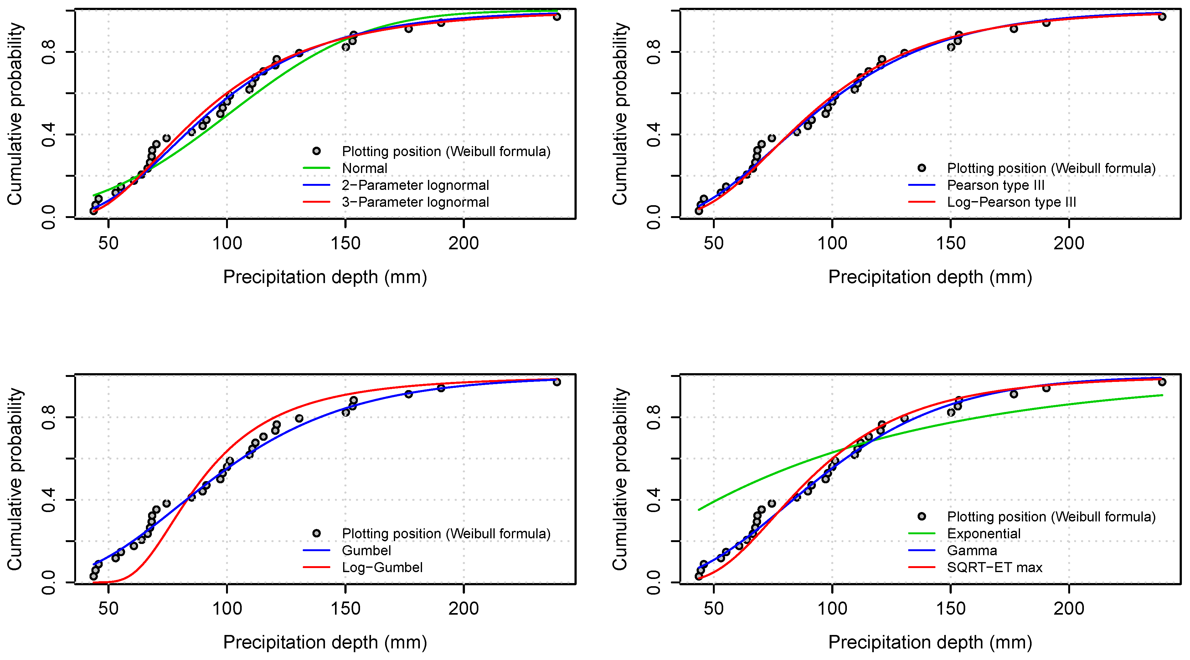
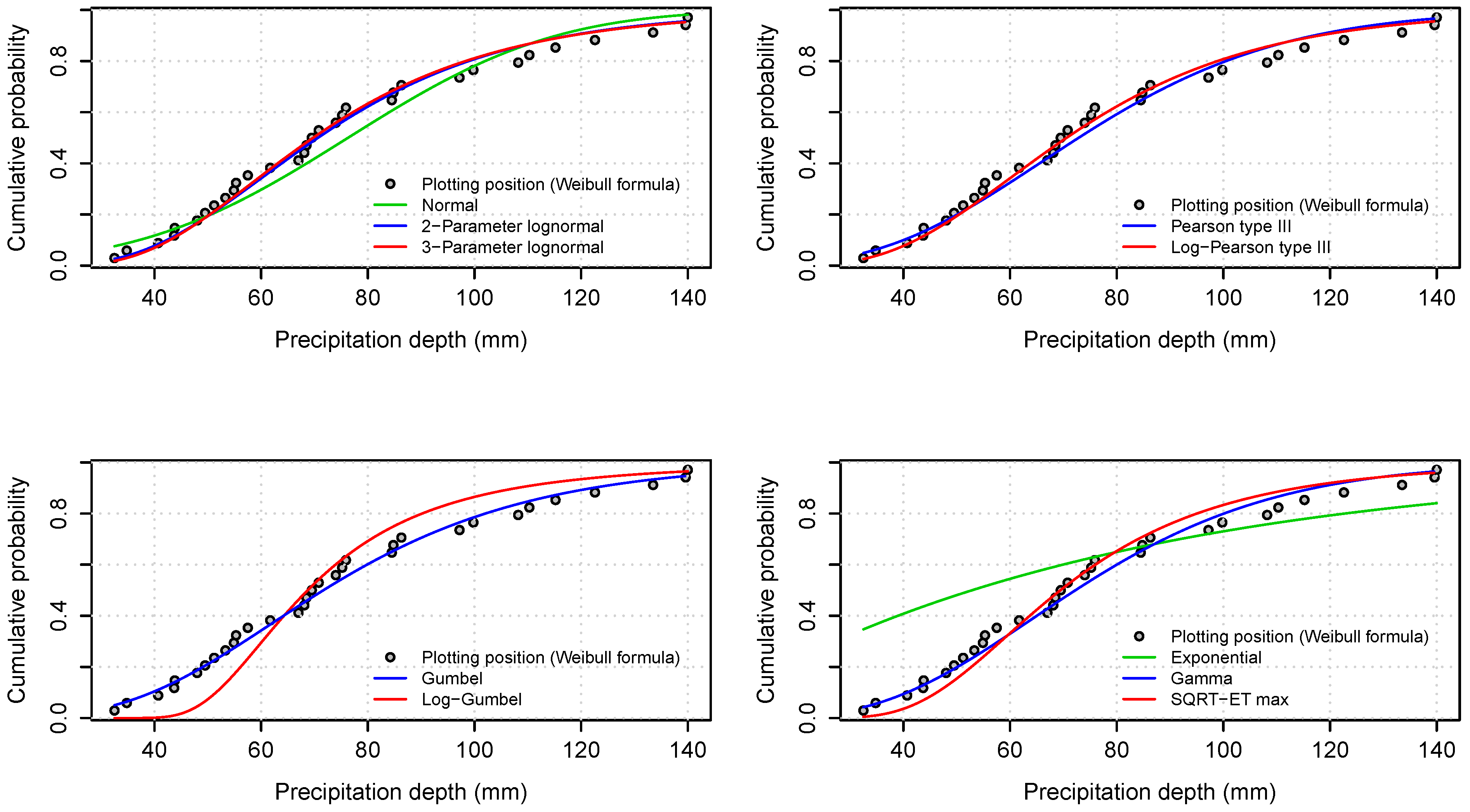
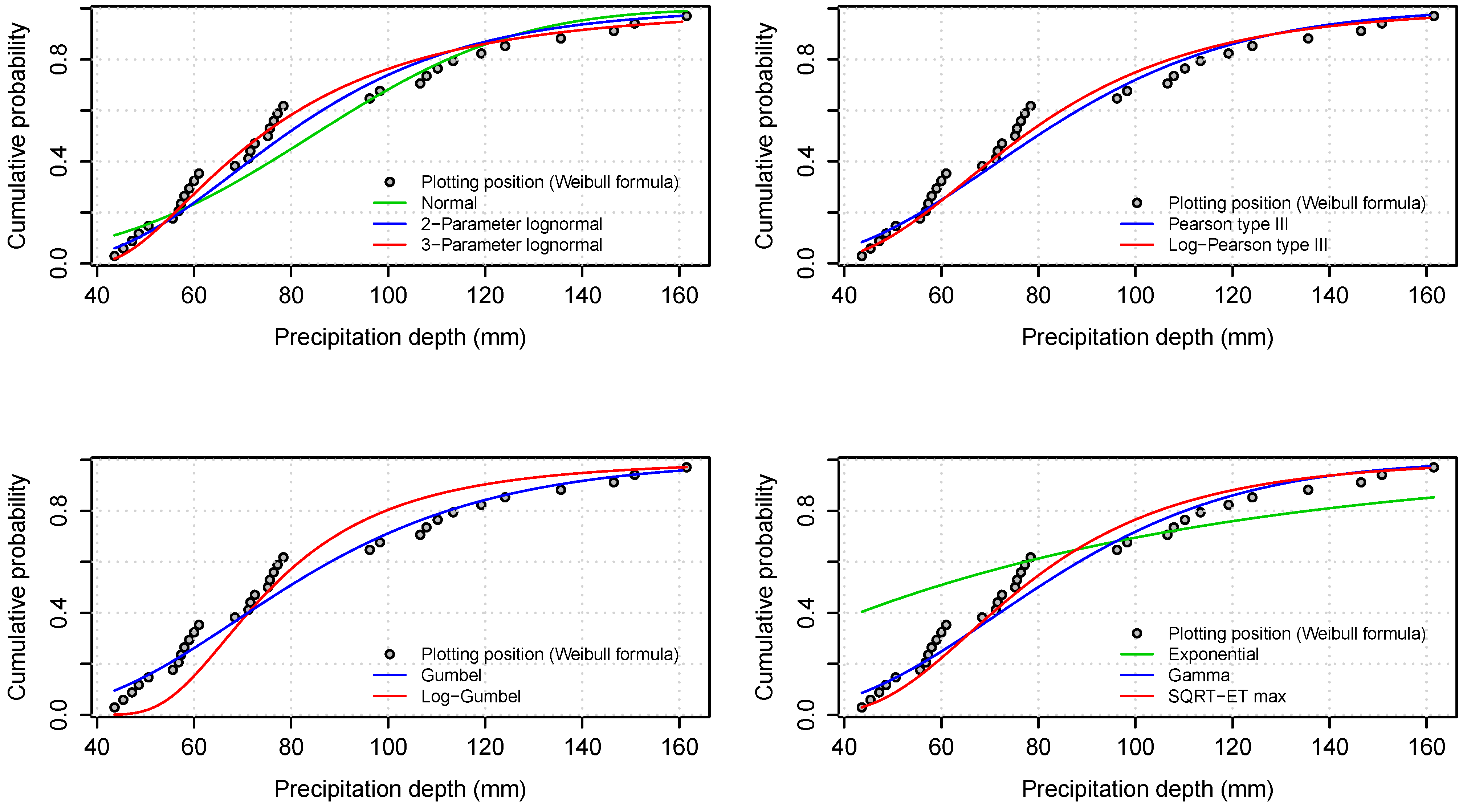
We carried out a study of the annual maximum 24 h rainfall data obtained from three weather stations. Modelling was performed using 10 different probability distribution functions, and the following results were obtained: (i) The selection of distribution functions for hydrological modelling requires a preliminary choice based on a test-fit validation criterion, including rainfall data from weather stations in the same area. (ii) Based on the three rainfall data sets and the climate area where the weather stations are located, two functions were found that should not be used for modelling; namely, the cumulative normal and exponential probability distribution functions were rejected by goodness-of-fit tests. (iii) A frequency analysis of the cumulative distribution functions was performed, which indicated that the best-performing distributions were the log-Gumbel and three-parameter log-normal for high return periods ($T>100$ years) and the Gumbel and three-parameter log-normal for low return periods ($T<50$ years). However, the use of the log-Gumbel is discouraged, as it has a high sensitivity, while the use of the SQRT-ET max and log-Pearson type III distributions cannot be discouraged, as they are known to perform well and have been commonly used in different countries (e.g., USA and Spain).

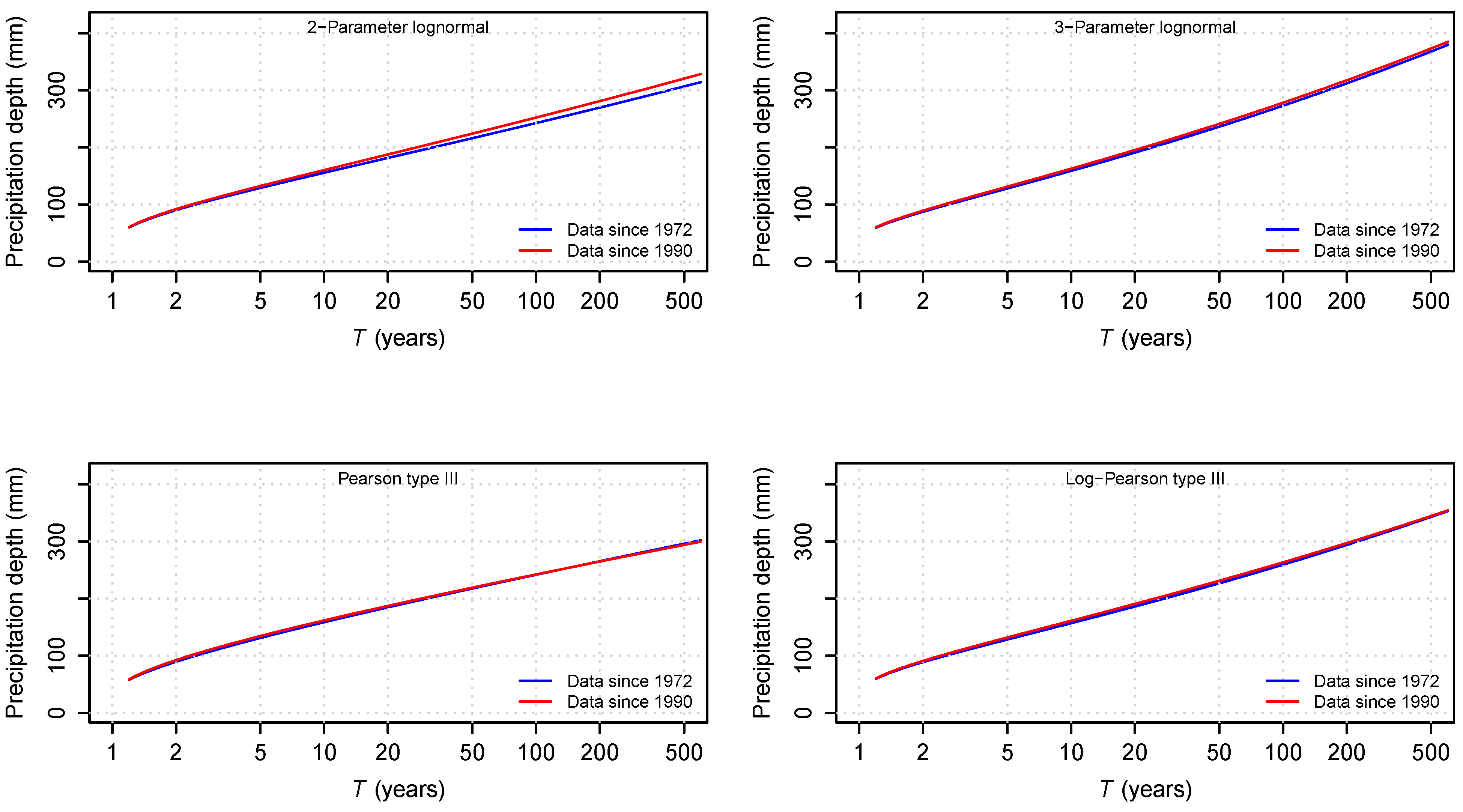
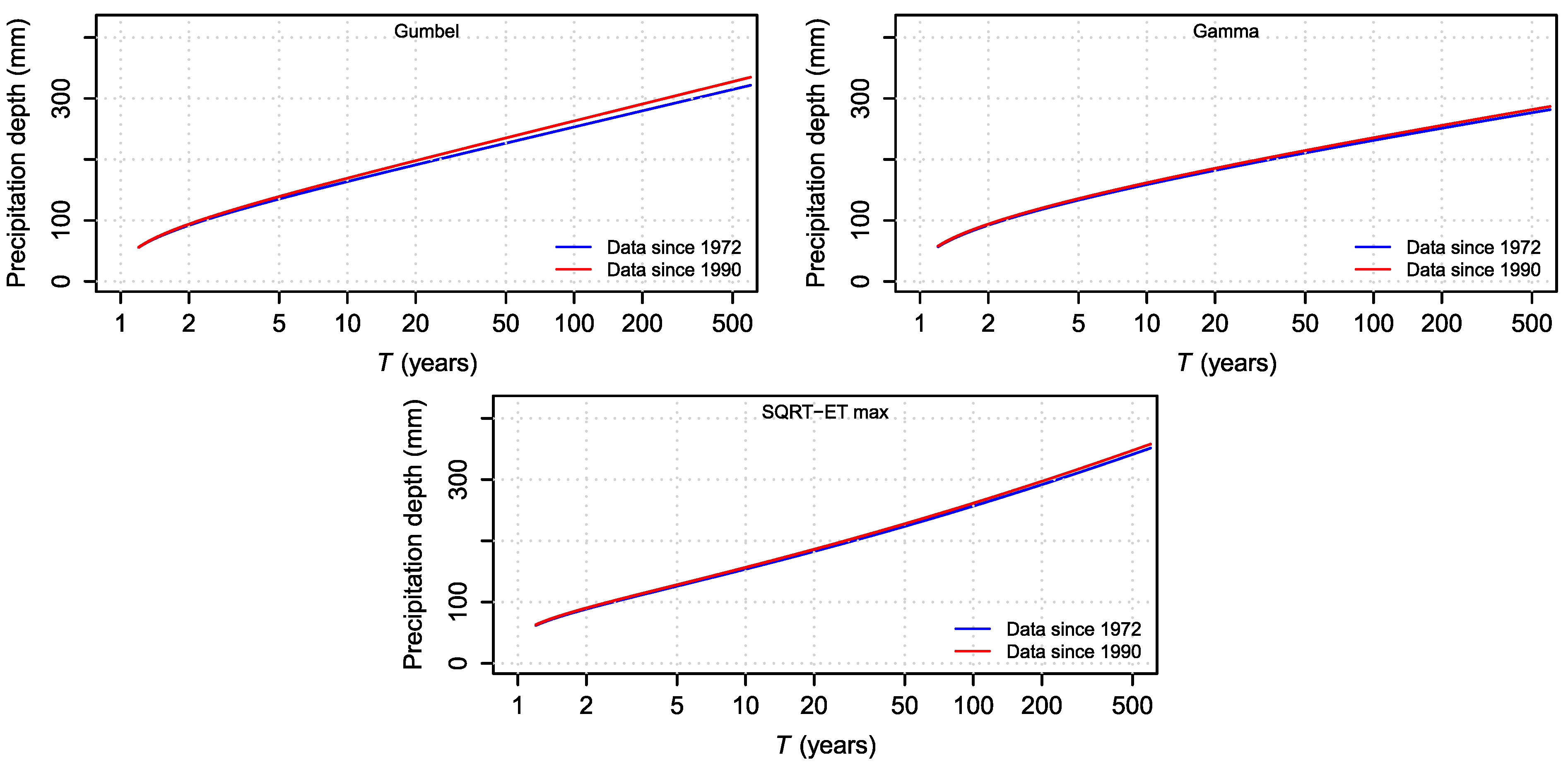
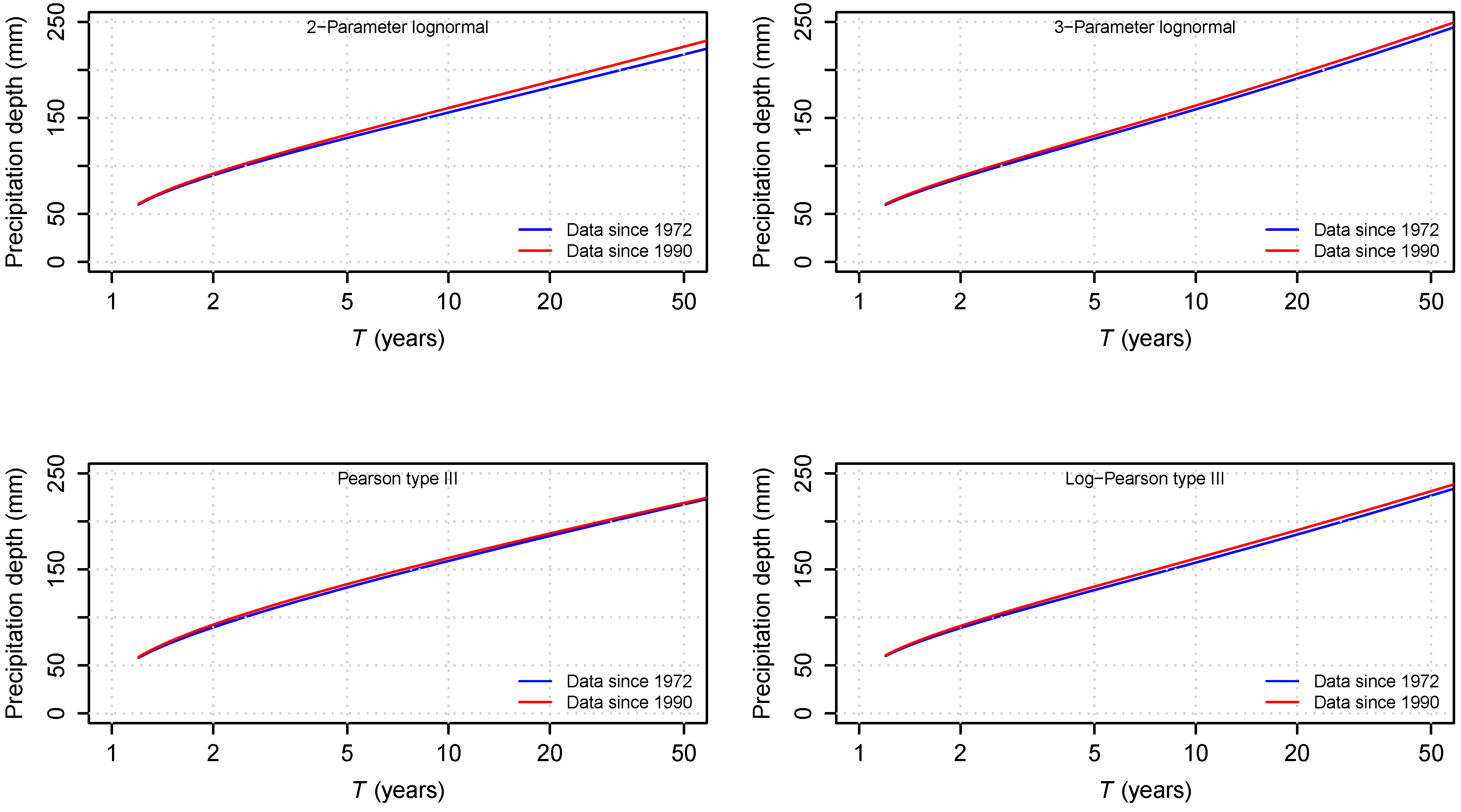
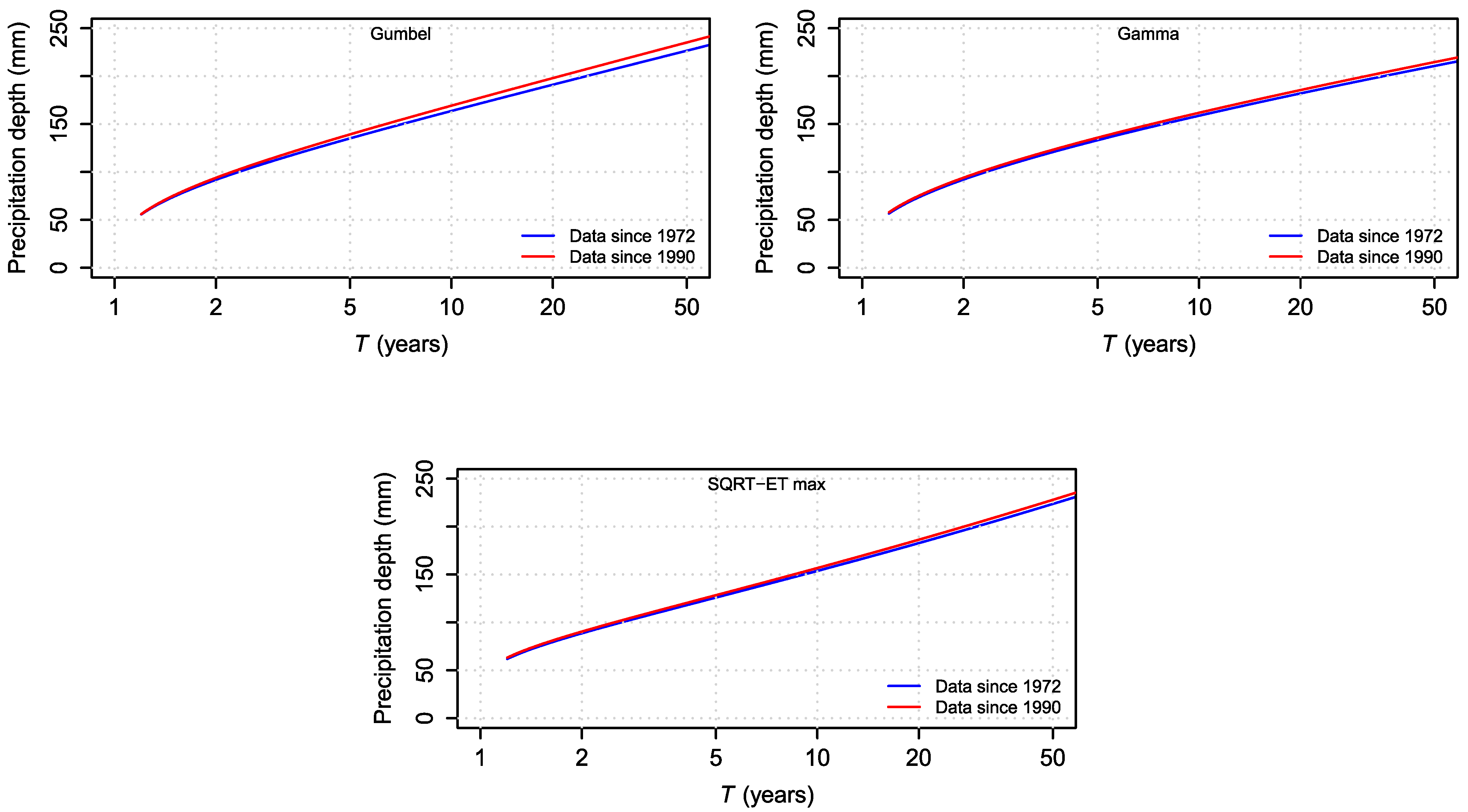
Furthermore, a study comparing data from the Castellar de la Frontera weather station since 1972 with data from the same station since 1990 was conducted in order to detect indicators of the effects of climate change on extreme precipitation events. We detected that the minimum possible value of the annual maximum 24 h rainfall is decreasing, while the annual maximum 24 h rainfall is increasing for the same return period T.

One of the requirements of the procedure adopted in this work is the need to test a high number of probability distribution functions, which a priori are recommended for the type of hydroclimatic variable analysed. The selection criteria for these candidate functions must be adapted to the new published findings, both to include new functions and to discard some of those that have been habitually used. In this sense, it is advisable to include candidate functions belonging to the Lindley family of distributions in future works.

References

1. Hossain, F.; Jeyachandran, I.; Pielke, R., Sr. Dam safety effects due to human alteration of extreme precipitation. Water Resour. Res. 2010, 46. [Google Scholar] [CrossRef]
2. Zhao, X.; Li, H.; Cai, Q.; Pan, Y.; Qi, Y. Managing Extreme Rainfall and Flooding Events: A Case Study of the 20 July 2021 Zhengzhou Flood in China. Climate 2023, 11, 228. [Google Scholar] [CrossRef]
3. Mailhot, A.; Duchesne, S. Design criteria of urban drainage infrastructures under climate change. J. Water Resour. Plan. Manag. 2010, 136, 201–208. [Google Scholar] [CrossRef]
4. Kuo, C.C.; Gan, T.Y. Risk of exceeding extreme design storm events under possible impact of climate change. J. Hydrol. Eng. 2015, 20, 04015038. [Google Scholar] [CrossRef]
5. Kang, W.; So, B.J.; Kim, S.; Lee, J.H.; Jang, E.K.; Kim, H.S. Update of Empirical Models for Predicting Specific Degradation in South Korea and Future Sediment Management Considering Climate Change. KSCE J. Civ. Eng. 2024, 28, 186–196. [Google Scholar] [CrossRef]
6. Greenwood, J.A.; Durand, D. Aids for fitting the gamma distribution by maximum likelihood. Technometrics 1960, 2, 55–65. [Google Scholar] [CrossRef]
7. Reich, B.M. Flood series compared to rainfall extremes. Water Resour. Res. 1970, 6, 1655–1667. [Google Scholar] [CrossRef]
8. Sangal, B.; Biswas, A. The 3-Parameter Log Normal Distribution and Its Applications in Hydrology. Water Resour. Res. 1970, 6, 505–515. [Google Scholar] [CrossRef]
9. Haan, C.T.; Allen, D.M. Comparison of multiple regression and principal component regression for predicting water yields in Kentucky. Water Resour. Res. 1992, 8, 1593–1596. [Google Scholar] [CrossRef]
10. Carey, D.I.; Haan, C.T. Using parametric models of runoff to improve parameter estimates for stochastic models. Water Resour. Res. 1975, 11, 874–878. [Google Scholar] [CrossRef]
11. Lone, S.A.; Sindhu, T.N.; Hassan, M.K.; Abushal, T.A.; Anwar, S.; Shafiq, A. Theoretical Structure and Applications of a Newly Enhanced Gumbel Type II Model. Mathematics 2023, 11, 1797. [Google Scholar] [CrossRef]
12. Reinders, J.B.; Munoz, S.E. Accounting for hydroclimatic properties in flood frequency analysis procedures. Hydrol. Earth Syst. Sci. 2024, 28, 217–227. [Google Scholar] [CrossRef]
13. Ye, X.; Garikapati, V.M.; You, D.; Pendyala, R.M. A practical method to test the validity of the standard Gumbel distribution in logit-based multinomial choice models of travel behavior. Transp. Res. Part Methodol. 2017, 106, 173–192. [Google Scholar] [CrossRef]
14. Lin, H.; Liu, L.; Zhang, Z. Hedging and Evaluating Tail Risks via Two Novel Options Based on Type II Extreme Value Distribution. Symmetry 2021, 13, 1630. [Google Scholar] [CrossRef]
15. Hou, Y.; Wang, X. Extreme and inference for tail Gini functionals with applications in tail risk measurement. J. Am. Stat. Assoc. 2021, 116, 1428–1443. [Google Scholar] [CrossRef]
16. Institute of Hydrology (Great Britain). Flood Studies Report: Hydrological Data; Natural Environment Research Council: Swindon, UK, 1975; Volume 4. [Google Scholar]
17. Ministerio de Fomento. Máximas Lluvias Diarias en la España Peninsular; Centro de Publicaciones, Ministerio de Fomento: Madrid, Spain, 1999; Available online: https://www.mitma.gob.es/recursos_mfom/0610300.pdf (accessed on 19 February 2024).
18. Casas, M.C.; Herrero, M.; Ninyerola, M.; Pons, X.; Rodríguez, R.; Rius, A.; Redaño, A. Analysis and objective mapping of extreme daily rainfall in Catalonia. Int. J. Climatol. 2007, 27, 399–409. [Google Scholar] [CrossRef]
19. Myhre, G.; Alterskjaer, K.; Stjern, C.W. Frequency of extreme precipitation increases extensively with event rareness under global warming. Sci. Rep. 2019, 9, 16063. [Google Scholar] [CrossRef] [PubMed]
20. Sun, Q.; Zhang, X.; Zwiers, F.; Westra, S.; Alexander, L. A Global, Continental, and Regional Analysis of Changes in Extreme Precipitation. J. Clim. 2021, 34, 243–258. [Google Scholar] [CrossRef]
21. Kendon, E.J.; Fischer, E.M.; Short, C.J. Variability conceals emerging trend in 100yr projections of UK local hourly rainfall extremes. Nat. Commun. 2023, 14, 1133. [Google Scholar] [CrossRef]
22. Del Jesus, M.; Diez-Sierra, J. Climate change effects on sub-daily precipitation in Spain. Hydrol. Sci. J. 2023, 68, 1065–1077. [Google Scholar] [CrossRef]
23. Meseguer-Ruiz, O.; Olcina Cantos, J. Climate change in two Mediterranean climate areas (Spain and Chile): Evidences and projections. Investig. Geográficas 2023, 79, 9–31. [Google Scholar] [CrossRef]
24. Cook, L.M.; McGinnis, S.; Samaras, C. The effect of modeling choices on updating intensity-duration-frequency curves and stormwater infrastructure designs for climate change. Clim. Chang. 2020, 159, 289–308. [Google Scholar] [CrossRef]
25. Yan, L.; Xiong, L.; Jiang, C.; Zhang, M.; Wang, D.; Xu, C.Y. Updating intensity–duration–frequency curves for urban infrastructure design under a changing environment. Wiley Interdiscip. Rev. Water 2021, 8, e1519. [Google Scholar] [CrossRef]
26. Crevolin, V.; Hassanzadeh, E.; Bourdeau-Goulet, S. Updating the intensity-duration-frequency curves in major Canadian cities under changing climate using CMIP5 and CMIP6 model projections. Sustain. Cities Soc. 2023, 92, 104473. [Google Scholar] [CrossRef]
27. Mínguez, R.; Herrera, S. Spatial extreme model for rainfall depth: Application to the estimation of IDF curves in the Basque country. Stoch Env. Res. Risk Assess 2023, 37, 3117–3148. [Google Scholar] [CrossRef]
28. WMO. Guide to Hydrological Practices Volume II: Management of Water Resources and Application of Hydrological Practices; WMO Report No 168; World Meteorological Organization: Geneva, Switzerland, 2009. [Google Scholar]
29. Maity, R. Statistical Methods in Hydrology and Hydroclimatology; Springer: Singapore, 2018; Volume 555. [Google Scholar] [CrossRef]
30. Raynal Villaseñor, J.A. Two-Parameters Log-Normal Distribution. In Frequency Analyses of Natural Extreme Events; Earth and Environmental Sciences Library; Springer: Cham, Switzerland, 2021. [Google Scholar] [CrossRef]
31. Singh, V.P. Three-Parameter Lognormal Distribution. In Entropy-Based Parameter Estimation in Hydrology; Water Science and Technology Library; Springer: Dordrecht, The Netherlands, 1998; Volume 30. [Google Scholar] [CrossRef]
32. Dodge, Y. Gamma Distribution. In The Concise Encyclopedia of Statistics; Springer: New York, NY, USA, 2008. [Google Scholar] [CrossRef]
33. Gumbel, E.J. The return period of flood flows. Ann. Math. Stat. 1941, 12, 163–190. Available online: https://www.jstor.org/stable/2235766 (accessed on 30 January 2024). [CrossRef]
34. Chow, V.T.; Maidment, D.R.; Mays, L.W. Applied Hydrology; McGraw-Hill: New York, NY, USA, 1988. [Google Scholar]
35. Gumbel, E.J. Les valeurs extrêmes des distributions statistiques. Ann. L’Inst. Henri Poincare-Anal. 1935, 5, 115–158. Available online: http://www.numdam.org/item/AIHP_1935__5_2_115_0.pdf (accessed on 30 January 2024).
36. Heo, J.H.; Salas, J.D. Estimation of quantiles and confidence intervals for the log-Gumbel distribution. Stoch. Hydrol. Hydraul. 1996, 10, 187–207. [Google Scholar] [CrossRef]
37. Bobee, B.B.; Robitaille, R. The use of the Pearson type 3 and log Pearson type 3 distributions revisited. Water Resour. Res. 1977, 13, 427–443. [Google Scholar] [CrossRef]
38. Pearson, K. Contributions to the mathematical theory of evolution. Philos. Trans. R. Soc. 1894, 185, 71–110. [Google Scholar] [CrossRef]
39. Huynh, N.P.; Thambirajah, J.A. Applications of the log Pearson type-3 distribution in hydrology. J. Hydrol. 1984, 73, 359–372. [Google Scholar]
40. Etoh, T.; Murota, A.; Nakanishi, M. SQRT-exponential type distribution of maximum. In Hydrologic Frequency Modeling; Springer: Dordrecht, The Netherlands, 1987; pp. 253–264. [Google Scholar] [CrossRef]
41. Ferrer, F.J. El Modelo de Función de Distribución SQRT et MAX en el Análisis Regional de Máximos Hidrológicos. Aplicación a Lluvias Diarias. Ph.D. Thesis, Universidad Politécnica de Madrid, Madrid, Spain, 1996. [Google Scholar]
42. Ministerio Para la Transición Ecológica y el Reto Demográfico. Gobierno de España. Agencia Estatal de Meteorología (AEMET). Available online: https://www.aemet.es/en/serviciosclimaticos (accessed on 15 February 2024).
43. Wuensch, K.L. Chi-Square Tests. In International Encyclopedia of Statistical Science; Lovric, M., Ed.; Springer: Berlin/Heidelberg, Germany, 2011. [Google Scholar] [CrossRef]
44. International Commission of Large Dams (ICOLD). Definition of a Large Dam. Available online: https://www.icold-cigb.org/GB/dams/definition_of_a_large_dam.asp (accessed on 15 February 2024).
45. Rodríguez González, C.A.; Rodríguez-Pérez, Á.M.; López, R.; Hernández-Torres, J.A.; Caparrós-Mancera, J.J. Sensitivity Analysis in Mean Annual Sediment Yield Modeling with Respect to Rainfall Probability Distribution Functions. Land 2023, 12, 35. [Google Scholar] [CrossRef]
46. Yuan, J.; Emura, K.; Farnham, C.; Alam, M.A. Frequency analysis of annual maximum hourly precipitation and determination of best fit probability distribution for regions in Japan. Urban Clim. 2018, 24, 276–286. [Google Scholar] [CrossRef]
47. González-Álvarez, Á.; Viloria-Marimón, O.M.; Coronado-Hernández, Ó.E.; Vélez-Pereira, A.M.; Tesfagiorgis, K.; Coronado-Hernández, J.R. Isohyetal maps of daily maximum rainfall for different return periods for the Colombian Caribbean Region. Water 2019, 11, 358. [Google Scholar] [CrossRef]
48. Elsebaie, I.H.; El Alfy, M.; Kawara, A.Q. Spatiotemporal Variability of Intensity–Duration–Frequency (IDF) curves in arid areas: Wadi AL-Lith, Saudi Arabia as a case Study. Hydrology 2021, 9, 6. [Google Scholar] [CrossRef]
49. Alam, M.A.; Emura, K.; Farnham, C.; Yuan, J. Best-fit probability distributions and return periods for maximum monthly rainfall in Bangladesh. Climate 2018, 6, 9. [Google Scholar] [CrossRef]
50. Olofintoye, O.O.; Sule, B.F.; Salami, A.W. Best–fit Probability distribution model for peak daily rainfall of selected Cities in Nigeria. N. Y. Sci. J. 2009, 2, 1–12. [Google Scholar] [CrossRef]
51. Kumar, R.; Bhardwaj, A. Probability analysis of return period of daily maximum rainfall in annual data set of Ludhiana, Punjab. Indian J. Agric. Res. 2015, 49, 160–164. [Google Scholar] [CrossRef]
52. Wagesho, N.; Claire, M. Analysis of rainfall intensity-duration-frequency relationship for Rwanda. J. Water Resour. Prot. 2016, 8, 706. [Google Scholar] [CrossRef]
53. Baghel, H. Frequency analysis of daily rainfall data of Udaipur district. Int. J. Agric. Eng. 2020, 13, 67–73. [Google Scholar] [CrossRef]
54. Basumatary, V.; Sil, B.S. Generation of rainfall intensity-duration-frequency curves for the Barak River Basin. Meteorol. Hydrol. Water Manag. Res. Oper. Appl. 2018, 6, 47–57. [Google Scholar] [CrossRef]
55. R Core Team. R: A Language and Environment for Statistical Computing; R Foundation for Statistical Computing: Vienna, Austria, 2023; Available online: https://www.R-project.org (accessed on 15 February 2024).
56. Témez, J.R. Facetas del cálculo hidrometeorológico y estadístico de máximos caudales. Rev. Obras Públicas 2003, 3430, 47–51. [Google Scholar]
57. Watt, E.; Marsalek, J. Critical review of the evolution of the design storm event concept. Can. J. Civ. Eng. 2013, 40, 105–113. [Google Scholar] [CrossRef]
58. Hussain, T.; Bakouch, H.S.; Iqbal, Z. A new probability model for hydrologic events: Properties and applications. J. Agric. Biol. Environ. Stat. 2018, 23, 63–82. [Google Scholar] [CrossRef]
59. Hamed, D.; Alzaghal, A. New class of Lindley distributions: Properties and applications. J. Stat. Distrib. Appl. 2021, 8, 11. [Google Scholar] [CrossRef]
60. Bakouch, H.S.; Hussain, T.; Chesneau, C.; Jónás, T. A notable bounded probability distribution for environmental and lifetime data. Earth Sci. Inform. 2022, 15, 1607–1620. [Google Scholar] [CrossRef]
61. Irshad, M.R.; Aswathy, S.; Maya, R.; Nadarajah, S. New One-Parameter Over-Dispersed Discrete Distribution and Its Application to the Nonnegative Integer-Valued Autoregressive Model of Order One. Mathematics 2023, 12, 81. [Google Scholar] [CrossRef]
Figure 1. Flow chart of the methodology. Only the main operations are shown.
Mathematics 12 01093 g001
Figure 2. Cumulative probability versus precipitation depth for the probability distribution functions at the Castellar de la Frontera weather station.
Mathematics 12 01093 g002
Figure 3. Cumulative probability versus precipitation depth for the probability distribution functions at the Almodovar reservoir weather station.
Mathematics 12 01093 g003
Figure 4. Cumulative probability versus precipitation depth for the probability distribution functions at the Jimena de la Frontera weather station.
Mathematics 12 01093 g004
Figure 5. Precipitation depth against return period for the probability distribution functions and T from 1.2 to 500 years at the Castellar de la Frontera weather station.
Mathematics 12 01093 g005
Figure 6. Precipitation depth against return period for the probability distribution functions and T from 1.2 to 500 years at the Almodovar reservoir weather station.
Mathematics 12 01093 g006
Figure 7. Precipitation depth against return period for the probability distribution functions and T from 1.2 to 500 years at the Jimena de la Frontera weather station.
Mathematics 12 01093 g007
Figure 8. Precipitation depth against return period for the probability distribution functions and T from 1.2 to 50 years at the Castellar de la Frontera weather station.
Mathematics 12 01093 g008
Figure 9. Precipitation depth against return period for the probability distribution functions and T from 1.2 to 50 years at the Almodovar reservoir weather station.
Mathematics 12 01093 g009
Figure 10. Precipitation depth against return period for the probability distribution functions and T from 1.2 to 50 years at the Jimena de la Frontera weather station.
Mathematics 12 01093 g010
Figure 11. Comparison between two-parameter log-normal, three-parameter log-normal, Pearson type III, and log-Pearson type III distributions for T from 1.2 to 500 years.
Mathematics 12 01093 g011
Figure 12. Comparison between Gumbel, gamma, and SQRT-ET max distributions for T from 1.2 to 500 years.
Mathematics 12 01093 g012
Figure 13. Comparison between two-parameter log-normal, three-parameter log-normal, Pearson type III, and log-Pearson type III distributions for T from 1.2 to 50 years.
Mathematics 12 01093 g013
Figure 14. Comparison between Gumbel, gamma, and SQRT-ET max distributions for T from 1.2 to 50 years.
Mathematics 12 01093 g014