
Simultaneous Bayesian Clustering and Model Selection with Mixture of Robust Factor Analyzers

1
School of Mathematics and Statistics, Northwestern Polytechnical University, Xi’an 710129, China
2
College of Statistics, Xi’an University of Finance and Economics, Xi’an 710100, China
*
Authors to whom correspondence should be addressed.
Mathematics 2024, 12(7), 1091; https://doi.org/10.3390/math12071091
Submission received: 29 February 2024
/
Revised: 29 March 2024
/
Accepted: 2 April 2024
/
Published: 4 April 2024
(This article belongs to the Special Issue Bayesian Inference, Prediction and Model Selection)
Abstract
:Finite Gaussian mixture models are powerful tools for modeling distributions of random phenomena and are widely used for clustering tasks. However, their interpretability and efficiency are often degraded by the impact of redundancy and noise, especially on high-dimensional datasets. In this work, we propose a generative graphical model for parsimonious modeling of the Gaussian mixtures and robust unsupervised learning. The model assumes that the data are generated independently and identically from a finite mixture of robust factor analyzers, where the features’ salience is adjusted by an active set of latent factors to allow a violation of the local independence assumption. For the model inference, we propose a structured variational Bayes inference framework to realize simultaneous clustering, model selection and outlier processing. Performance of the proposed algorithm is evaluated by conducting experiments on artificial and real-world datasets. Moreover, an application on the high-dimensional machine learning task of handwritten alphabet recognition is introduced.
Keywords:
Bayesian inference; feature selection; mixture of factor analyzers; robust clustering; structured variational BayesMSC:
62H30; 62F15; 62H221. Introduction
Finite Gaussian mixture models are powerful tools for modeling distributions of random phenomena. They are widely used for unsupervised classification tasks and lay the foundation for many deep learning-based clustering algorithms, e.g., [1,2]. However, competitive performance of the Gaussian mixture model cannot be expected on high-dimensional datasets due to the curse of dimensionality [3]. The impact of redundancy and noise can degrade the model’s interpretability and efficiency, which is crucial in many application fields such as molecular biology and the clinical medicine [4]. Since the intrinsic dimensions of high-dimensional data are usually much less than their original feature space, it is possible to improve the clustering performance via dimension-reduction methods [5].
Feature-selection approaches are designed to retain a subset of features that are informative and discriminant for clustering. The two-stage methods implement the feature selection and clustering separately, which consider the preselected features as input without regarding the subsequent clustering algorithms [6,7]. But as choosing the feature subset and clustering are highly dependent problems, to circumvent the loss of information, incorporating the feature selection in the clustering algorithms and constructing an integrated objective function is suggested [3,4]. Pan and Shen [8] proposed a penalized likelihood approach for unsupervised feature selection where they used an penalty to shrink the component means. A similar approach was also suggested in [9], where the feature-selection consistency via the penalization was further studied. However, as both approaches are highly dependent on the choosing of penalization parameters, cross-validation or criterion-based model selection is required to tune the parameters.
A different stream of research casts the feature selection as parameter-estimation problems [4,10,11,12], where the random variable “feature saliency” is introduced to quantify the relevance of features to class assignment. This approach is efficient as neither combinatorial search through the feature subsets nor tuning of parameters is required. The feature selection and the clustering can be performed simultaneously in a principled and automatic way. Zhang et al. [13] extended this method to the Student’s t mixture model, which has higher tolerance to outliers and therefore is more robust for clustering and feature selection. As an extension to the work of Zhang et al., Sun and Zhou [14] made a full-Bayesian treatment for the model and proposed the structured variational Bayesian (VB) approach, which takes into consideration the estimation uncertainty of all model parameters and can deliver a tighter bound to the marginal likelihood than the mean-field approximated VB algorithms. Their model was extended further in [3] to consider the class-specific feature saliency for Bayesian feature selection.
Feature-selection approaches commonly assume that the features are conditionally independent given the latent class variable, which is equivalent to adopting a diagonal component covariance matrix structure in the Gaussian mixture model. While this assumption greatly facilitates computational efficiency, it can be easily violated in real-world datasets [15]. For the linear regression analysis, Fan et al. [16] conducted a synthetic study indicating that when the covariates are highly correlated exact recovery of the active set from the solution path of LASSO will be difficult. For classification, as has been mentioned in [17], ignoring the dependence relationship across features may undermine the reliability of the algorithms and lead to misleading conclusions about the features’ salience.
In [18], the local independence assumption for the Gaussian mixture model was relaxed by a block-diagonal specification of the component covariance matrix, where the features are partitioned into several disconnected groups in each class. However, as the total number of block-diagonal structures increases as the Bell number [19], searching for the optimal model can be difficult, especially in the high-dimensional cases. Galimberti and Soffritti [18] proposed a hierarchical aggregative strategy based on the BIC criterion to perform a nonexhaustive search of the structures. But this method cannot promise to find the optimal model. Ruan et al. [20] extended the graphical LASSO method to the context of the Gaussian mixture model and proposed a penalized likelihood approach for a sparse solution of the component covariance matrices. But the penalization parameters still need to be selected.
Different to the block-diagonal specification, the model of mixture of factor analyzers assumes a factor analysis-based decomposition structure for the component covariance matrices, where the local dependence between features is explained by a few latent factors [21,22,23,24]. Typically, the number of factors for each component needs to be specified in advance of the model fitting or the model-selection criterion used to select the optimal number of factors. However, while presetting of the number may lead to over-fitted or over-simplified models, conducting exhaustive searches over the model space is computationally expensive. The shrinkage prior methods were proposed to achieve an automatic latent dimension reduction. Wang and Lan [25] imposed automatic relevance determination prior [26] on the factor loading matrices. Multiplicative Gamma process shrinkage priors [27] in the infinite factor analysis was used by Murphy et al. [28]. They also suggested an adaptive Gibbs sampling algorithm where the factors with negligible loadings are removed gradually during the iterations. Therefore, the computational efficiency can be improved.
In this paper, we develop further the Student’s t mixture model of Sun and Zhou [14] for Bayesian clustering and feature selection to tackle the cases where features are correlated in the mixture component. While the model in [14] defines the feature saliency under the local independence assumption, we introduce the factor-adjusted feature saliency, where the salience of each feature is evaluated by conditioning on the latent factors. Taken as a whole, the extension produces parsimonious, flexible and robust modeling for the mixture of factor analyzers. Moreover, motivated by the Bayesian model selection method in [29] for the linear regression analysis, instead of using the shrinkage priors, we propose an automatic inference scheme for the number of factors by introducing the random variable of factor activity. Then, the problems of feature selection, latent dimension reduction, outlier processing and clustering can be integrated together as the inference for a Bayesian hierarchical latent variable model. We continue the work in [14] to adopt a full Bayesian treatment, where proper prior distributions are assumed for the model parameters. The structured VB inference framework that improves the evidence lower bound (ELBO) for the proposed model is presented, where a “drop-out” sampling technique [30] can be applied immediately to ease the computation.
The rest of this paper is organized as follows: In Section 2, we introduce the Student’s t mixture model proposed by Sun and Zhou [14], which has provided the base of our study. In Section 3, we develop the proposed mixture of robust factor analyzers, which is present as a hierarchical latent variable model for Bayesian inference. In Section 4, the structured VB inference framework for the proposed model is established. Section 5 justifies the performance of the developed model and algorithm on the synthetic data and presents the evaluation results based on some real-world datasets. Section 6 concludes this paper, points out the limitations and suggests future research directions.
2. The Student’s t Mixture Model for Feature Selection
We present the proposed hierarchical latent variable model starting from the Student’s t mixture model defined in [14]. Denote the set of i.i.d. observations as , where is the d-dimensional feature data for the nth individual. The finite mixture model for clustering assumes that the data for each individual are generated from a class-specific distribution but with the class label missing, then it marginally follows a finite mixture distribution. Throughout the paper, we denote the number of mixture components or equally the number of classes as K. The latent class label for the nth individual is denoted as which takes value in . The clustering is realized by assigning each individual the class label where it has the highest posterior probability of belonging.
The Student’s t mixture model given in [14] assumes that the features are conditionally independent given the hidden class label and each follows a Student’s t distribution. Moreover, the relevance or irrelevance of feature to data separation is taken into account by introducing the Bernoulli latent variables , which gives the mixture density of as
is the density function of the Student’s t distribution with mean, precision and degrees of freedom as , and v, respectively. For , , if , then the lth feature is relevant to the class assignment; if , then the lth feature is irrelevant and follows a common distribution independent of the class assignment. For , the parameter ( and ) is the mixing proportion of class k. Let denote the set of unknown parameters in model (1), where , , and .
The prior distribution of is given by
where the ’s are assumed to be mutually independent. The parameter for the Bernoulli distribution of is called the feature saliency [4] of the lth feature. It measures the importance of the feature for class assignment and is estimated to realize a “soft” feature selection. Denote .
The observed-data likelihood function can be obtained by integrating over the latent variables in model (1), which gives
where . Statistical inference directly on the observed-data likelihood is difficult. In [14], the VB inference method was adopted where the complete-data likelihood is given by
At the right-hand side of (4), is the Kronecker delta function. The latent variables are introduced by noting that the Student’s t distribution can be written as a convolution of a Gaussian and a Gamma distribution [3,14]. It follows that
and
represents the Gaussian density function with mean and precision and is the Gamma density function
3. Towards the Mixture of Robust Factor Analyzers
To tackle the cases where features are correlated in the mixture component, we relax the local independence assumption in [14] by specifying for each class a latent factor model. Specifically, for class k, we introduce the latent factors , where ’s are i.i.d. from the distribution and is the number of latent factors. After conditioning on , the features are assumed mutually independent within the class, which corresponds to a modification of model (1) as follows:
where are the factor loadings for the lth feature in class k. Denote and where . In model (8), indicates the relevance of the lth feature to class assignment after adjustment by the latent factors. Correspondingly, that defines the distribution of in (2) represents the factor-adjusted feature saliency.
Typically, in each local factor model, the latent dimensions need to be specified. With overly high dimensions, the model may over-fit the data, yielding poor interpretations and hardening the computation, while with low and inadequate dimensions, the model may not be flexible enough to capture the correlations between features in each class. To enable an automatic determination, we treat the problem as another feature-selection task, but now the “features” become the latent factors. Starting from a sufficiently large , we introduce in class k the Bernoulli latent variables , where with indicating that the factor is active and inactive. Model (8) then becomes
where and we denote . When ’s all equal zero, the model reduces to the Student’s t mixtures of model (1).
The prior distribution of is given by
where we have assumed prior independence between the entries of . Denote and . In accordance with the concept of feature saliency, we call the factor activity. It is the probability that the jth factor in class k is active. The problem of finding latent dimensions then can be cast as a parameter-estimation problem, i.e., the estimation of .
Our modeling of to select the active factors in each class is inspired by the normal-zero model proposed in [29], which introduces the indicators to select automatically the important covariates in linear regression. The difference is that we have defined the indicators as latent variables for each individual, while the normal-zero model introduces the indicators as model parameters. In our model, the parameters that define the Bernoulli distributions of the indicators are the key quantities for model selection and will be inferred under a Bayesian inference framework, while following the normal-zero model are treated as hyper-parameters and typically need to be specified.
Note that the conditional probability of (9) defines a mixture of robust factor analyzers. The factor model for class k can be written as
where is the factor loading matrix. Denote , and . The latent factors follow the distribution of , where is the identity matrix of order . The distributions for and are defined in (2) and (10), separately. , where ’s are mutually independent given and
By introducing the latent variable distributed according to (6), we have
The complete-data likelihood for the proposed hierarchical latent variable model, where can be factorized as
where
corresponding to a modification of conditional probability (5) for the Student’s t mixture model.
In the following, we denote the set of latent variables as where . Then, the complete-data likelihood for the whole dataset can be written as
Full Bayesian treatment to the latent variable model requires specification of the prior distributions associated with the model parameters. We assume that
and
where represents the Beta density function
and
is the Dirichlet density. In the above specifications, the conjugate priors are used. The parameters in the priors, including , , , , , , , , and where and , are considered as hyperparameters. It is noticeable that we do not assume any prior for the degrees of freedom ’s and ’s. Since there are no conjugate priors, we follow the practice in [3,14] to seek for the point estimates for them.
4. Inference on the Model
4.1. Brief Introduction to VB Method
To infer from the posterior distribution of the latent variables and the parameters, computation of the evidence is required. However, the computation involves integration over the latent variables and the parameters, which is intractable for our model. In this paper, we resort to the VB method for model inference. It is designed to maximize a lower bound of . Assuming posterior independence between the latent variables and the parameters, the evidence lower bound (ELBO) is defined by
where and are auxiliary posteriors for the latent variables and the parameters, respectively. A coordinate ascent search method [31] can be applied to iteratively maximize the ELBO. At the tth iteration, it implements the VB expectation (VB-E) step and the VB maximization (VB-M) step as follows:
4.2. Tree-Like Factorization of the Auxiliary Posterior
In this paper, we apply the tree-like factorization proposed in [3,14] to the auxiliary posterior of the latent variables. The resultant structured VB method can be viewed as a partially collapsed VB [32], which can reach a tighter lower bound for than the mean-filed approximated VB method [13].
As the observations are mutually independent, has the form
Tree-like factorization assumes that the auxiliary posterior can be factorized as
As entries of the noise term in the local factor model are assumed to be mutually independent, can be further factorized as
Different from [3,14], we do not keep the posterior dependence of on and when the auxiliary posterior of is assumed to be independent of , though the closed forms of the posteriors are available when retaining the dependencies. We found that the above specifications lead to more robust inference results. As in [29,33], we assume a full factorization for , i.e.,
Additionally, the auxiliary posterior is assumed to be its full factorized form
For ease of exposition, we use n, l, j and k in the following to denote the index of the individual, the feature, the latent factor and the class, respectively. We omit the iteration indexes and and without loss of generosity deliver the update during one iteration of the algorithm. We use to denote the expectation operation with respect to the current auxiliary posteriors.
4.3. Auxiliary Posteriors of the Latent Variables: VB-E Step
The VB-E step updates the auxiliary posterior of the latent variables following the factorizations of (25) and (26).
(i) : Through some mathematical manipulations (see the Supplementary Materials for the details), we obtain
where
and . Note that
where is the precision of posterior and is the precision of . We denote the trace operator as and the Hadamard product operator between two matrices as ⊙.
In the sequel, we use and to distinguish between the expectations regarding and . As with the property of Gamma distribution, we obtain
where is the digamma function.
(ii) : Define
Then, can be obtained by
and . Denote and .
(iii) : The posterior is multivariate Gaussian with precision matrix and mean vector as
where
(iv) : The posterior can be obtained by
and , where
with . The expectations in (37) are taken by fixing . Denote and .
When posterior independence is assumed between and or is observable as in the regression models of [29,33], can be derived analytically and the expectations in (30) regarding can be obtained in closed form using the results:
However, the computation in high-dimensional cases is obstructed as it involves multiplication and inversion of large-scale matrices.
The sparse property of the indicator vector motivates us to resort to a “drop-out” sampling scheme [30], where the conditioning of on does not influence the efficiency of the algorithm. Specifically, we keep a random sample from at each iteration of the algorithm and use it as an imputation for to update the remaining auxiliary posteriors. During this process, the connections to the latent factor with smaller have higher chance of drop out. Simplification of the computation can be realized, for example, in Equation (30),
where the latent dimensions to be tackled are reduced due to the sparse property of the random sample . For the multiplication and inversion computations, only the entries of vector or matrix corresponding to need to be involved.
To obtain a random sample from , we update the entries of one by one through a single turn of Gibbs sampling, where the sampling probability for has the form in (37) but with the expectation replaced by the current imputation of .
(v) : To update , we define the quantity
Then,
4.4. Auxiliary Posteriors of the Parameters: VB-M Step
The VB-M step updates the posterior for the parameters following the factorization in (27). Through mathematical manipulation (see the Supplementary Materials for the details), we have
where
The posterior is given by
where
The posteriors and are given by
where
In addition, the posteriors and are updated as
where
The degrees of freedom can be obtained by solving the nonlinear equation
Similarly, can be obtained by solving
4.5. Algorithm
The developed structured VB algorithm is summarized in Algorithm 1. The optimization process can be monitored via the ELBO (21). The computation of the ELBO is detailed in Appendix A.
| Algorithm 1 Proposed Structured VB Algorithm for Robust Clustering and Model Selection |
|
We apply K-mean clustering for initialization of the VB algorithm and initialize a large p for the latent dimensions of the K local factor models. At each iteration, we randomize the updating order of ’s in the Gibbs sampling step to avoid co-adaptation. To further accelerate the algorithm, we make the number of factors adaptive. The empirical estimator of factor activity, i.e.,
is computed at the end of each iteration. If , then we remove the jth latent factor from the kth local factor model. The pruning is carried out after a burn-in period of the algorithm.
4.6. Interpreting the Model
The expectation of feature saliency can be used to show the informative degree of features after being adjusted by latent factors, which is given by
In addition, the expectation of factor activity can be applied to evaluate the explanatory power of latent factors in each class, which can be obtained as
We also consider the reconstruction performance of the proposed algorithm. The centroid of each class is estimated by
where , and . Then, reconstruction for the nth individual in class k can be computed as
where and is obtained from the VB-E step after the algorithm converges.
5. Experiment Study
5.1. Experiments on Synthetic Data
In this section, we justify the developed model and the structured VB algorithm using controlled experiments. We continue the experiments in [14] with the same synthetic data where the features were generated independently in each component. An additional set of data was generated where we imposed correlation between features within the mixture component. The proposed model and algorithm was compared with the semi-Bayesian clustering model and algorithm in [10], called varFnMS, in which a finite mixture of Gaussian is adopted and a mean-field VB is applied and compared with the full-Bayesian model and algorithm in [14], denoted varFnMS-T, which is based on the mixture of Student’s t distribution and uses the structured VB algorithm.
The synthetic data in [14] contain 800 data points from four well-separated classes. The data are 10-dimensional with two influential features located around the class centers , , and with identity covariance matrices in each class. The remaining eight “noisy” features were sampled from . We made randomly of the data outliers by adding noises sampled uniformly from . The features are mutually independent in each class, which is consistent with the assumption underlying varFnMS and varFnMS-T. In the additional set of data, the local independence assumption is violated. We assigned a four-factor model for class 1, a two-factor model for class 2, a one-factor model for class 3 and no factor in class 4. The mean vector of each factor model remained the same as that in the “locally independent” data. The factor loading matrices were generated randomly with each entry from . The noise term in each class was generated from .
The proposed algorithm, denoted as varFnMS-TFA, the varFnMS and the varFnMS-T were carried out twenty times, separately. The number of clusters K was set as four. The K-mean clustering algorithm was used to initialize the posterior . The feature saliency and factor activity were both initialized as . The hyperparameters , and were set to be and was set as the empirical mean of the feature data. We assumed a nine-factor model for each class at the beginning and initialized the posterior means of the latent factors by sampling from . The algorithm terminates when the difference of the ELBO between two consecutive iterations is less than or the maximum number of iterations () is reached. To avoid the “label switching” problems, we labeled the obtained clusters from the twenty repeated experiments by matching with the true classification of the data.
The ELBO reached and the classification error rate comparing the clustering with the original grouping of the data via the three algorithms with the two synthetic datasets are presented in Table 1. For the dataset where features are mutually independent within class, the classification accuracy of varFnMS-TFA is slightly higher than the other two algorithms, but the difference is not evident. For the dataset generated with correlated features, the proposed algorithm shows significantly higher accuracy than the other two algorithms under the local independence assumption. Moreover, the ELBO reached via varFnMS-TFA is the highest on average in both datasets and the discrepancy is enlarged where the features are locally correlated. As seen in Figure 2, it successfully captures the correlation across features through the latent factors.
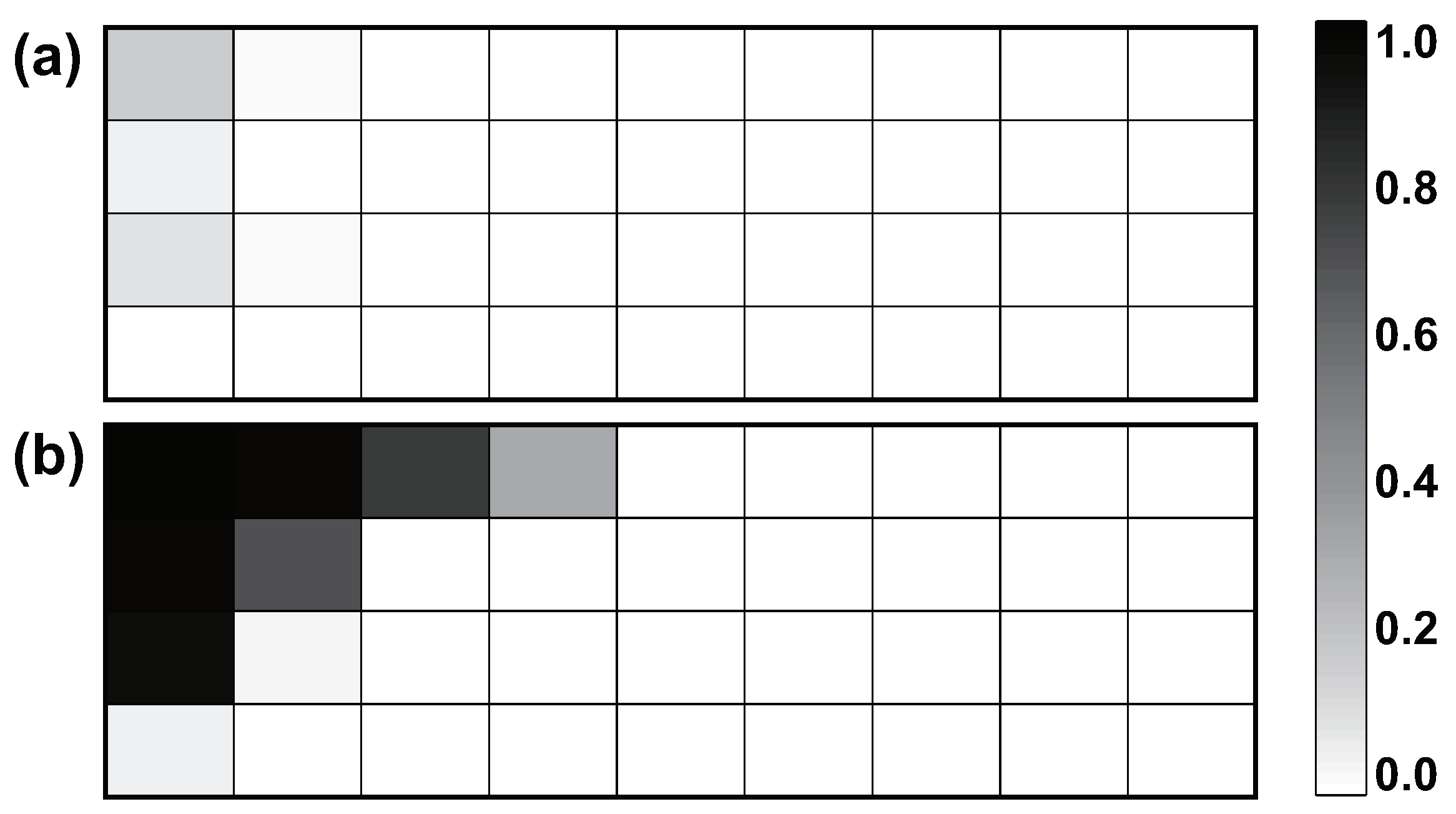
The estimated factor activity in each class by the proposed algorithm (averaged over the twenty repeats) for the two synthetic datasets is presented in Figure 2. Generally, the algorithm recovers the ground truth in both datasets. It can be seen in subplot (a) that there is no significantly active factor across the four classes for the “locally independent” data and the true pattern of factor activity in the “locally correlated” data is recovered as shown in subplot (b).
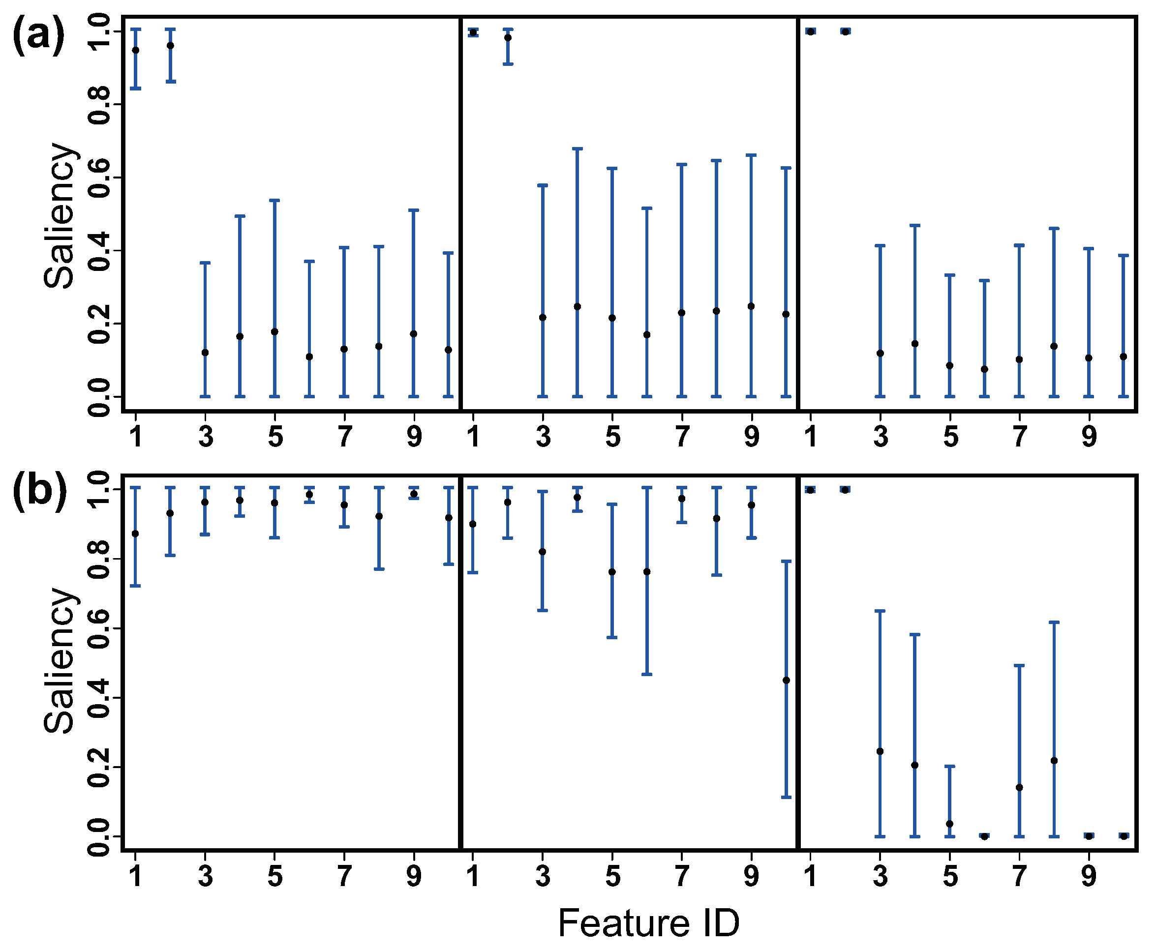
Figure 3 compares the estimated feature saliency for the two synthetic datasets. As shown in subplot (a), the three algorithms make the same good estimation on the feature saliency when the features are independent within class. But when the dependence relationship is imposed, the proposed algorithm shows apparently different behavior from the other two algorithms as shown in subplot (b). While varFnMS and varFnMS-T estimate the salience of a feature that could be confounded by the other features, varFnMS-TFA gives the factor-adjusted feature saliency, where the confounding effects are resolved by the latent factors.
In Table 2, the estimated class centroids in the two synthetic datasets (averaged over the twenty repeats) are present. When features are generated independently within class, the three algorithms exhibit comparable performance and recover the real centroids approximately. But with correlations imposed, the estimation accuracy by varFnMS or varFnMS-T is apparently degraded. In class 1, 2 and 3, they misestimate the means of the first two features that are salient and the variations of estimation are significantly enlarged compared with the results of varFnMS-TFA. In comparison, the varFnMS-TFA algorithm that considers the local dependence relationships gives more accurate and stable estimation results.
5.2. Experiments on Real Datasets
In this section, we apply the proposed model on the benchmark datasets: Iris, Olive, Wine and WDBC. The Iris dataset is obtained from the R package “datasets”. Olive is the Italian olive oil dataset and Wine the Italian wine dataset. They are both obtained from the R package “pgmm”. WDBC is the Wisconsin diagnostic breast cancer dataset downloaded from the UCI machine learning repository (https://doi.org/10.24432/C5DW2B; accessed on 26 May 2023). For each dataset, we repeated each algorithm ten times and retrieved the result with the highest value on ELBO. We set the initial dimensions of latent factors for each dataset as , where d is the number of features in the data. Table 3 presents the basic information for the four datasets and the classification error obtained. There is a significant decrease on the classification error for the Olive data and a slight improvement on the results for Iris and WDBC when using the proposed algorithm. The exception goes to the Wine data, where the proposed algorithm gives results slightly inferior to varFnMS-T.
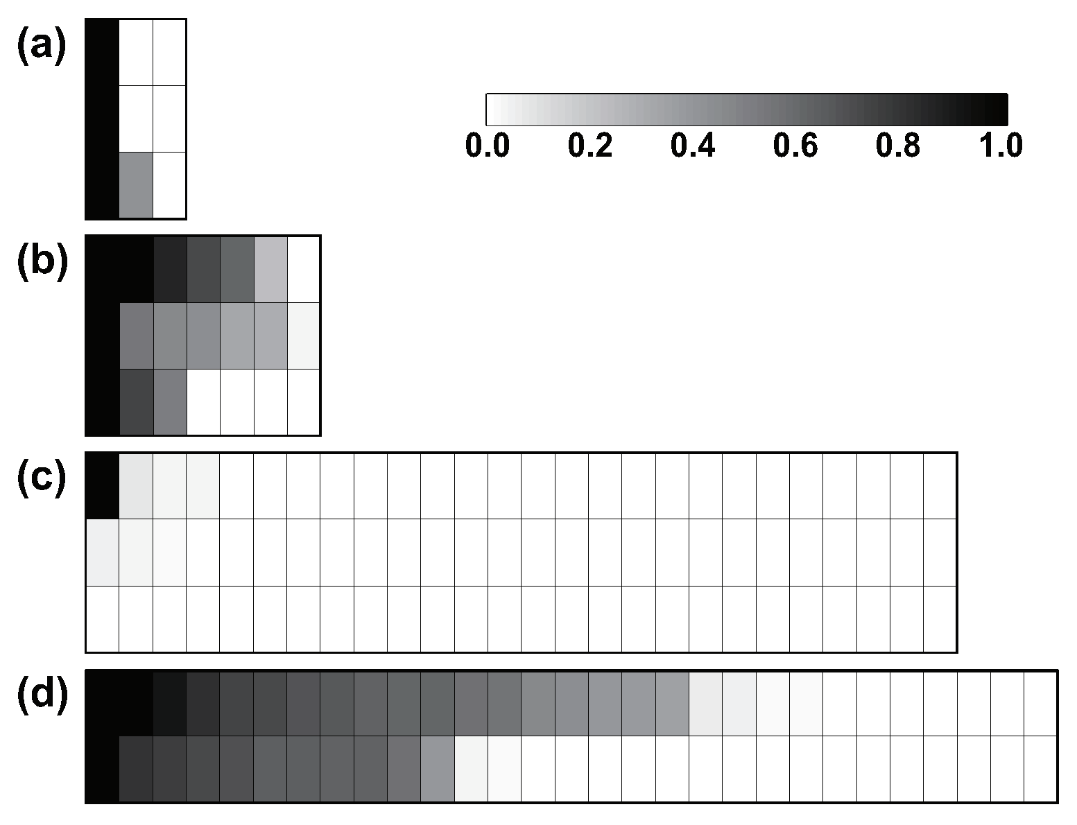
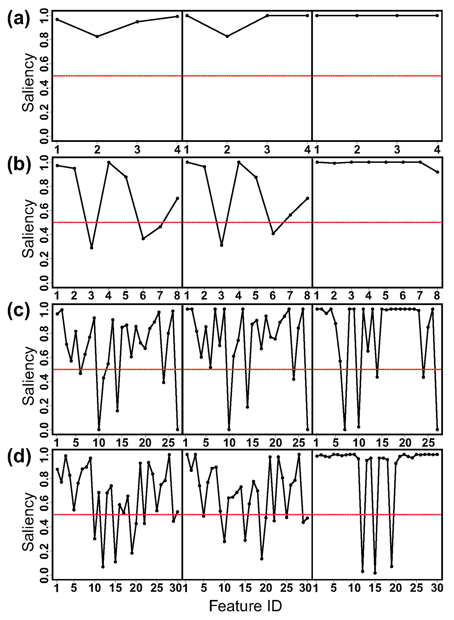
Figure 4 and Figure 5 show the factor activity and feature saliency for the four benchmark datasets. It can be seen from Figure 4 that strong factor activity is detected in Iris, Olive and WDBC data. As shown in Figure 5, the patterns of estimated feature saliency are noticeably changed when applying the proposed algorithm. The combined results indicate that the correlation between features could interfere with our decision about the features’ relevance and the classification of data.
5.3. Application on Handwritten Object Recognition
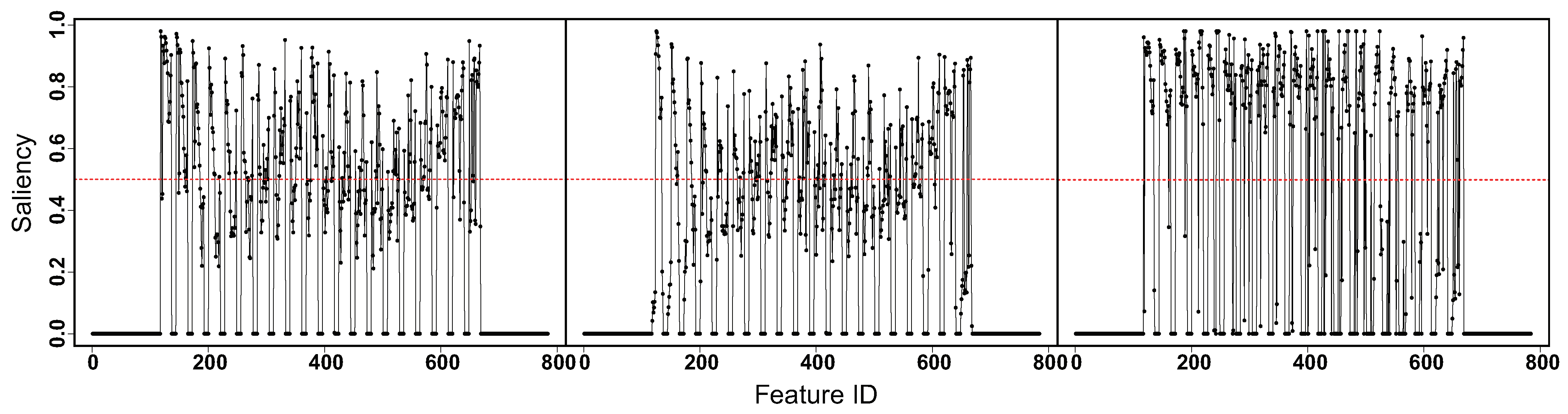
In this section, we apply the developed algorithm to the machine learning task of handwritten alphabet recognition. The handwritten alphabet dataset is obtained from the Kaggle webpage (https://www.kaggle.com/datasets/sachinpatel21/az-handwritten-alphabets-in-csv-format/data; accessed on 26 May 2023). It contains more than 370,000 images for the English alphabets (A–Z). The images are gray-scale in the size of pixels. We focus on separation of the handwritten alphabets A, B and C and reserve randomly 200 images for each of the alphabets. As the variability of some pixels in the image of an alphabet is exactly zero, we may encounter the singularity problem during iterations of the clustering algorithms. Therefore, pre-processing was implemented on the data as detailed in Appendix B. In the proposed algorithm, the initial number of latent factors was set as fifty for each class. The three algorithms attain the same classification error rate as 0.16. The patterns of feature saliency estimated via varFnMS, varFnMS-T and the proposed algorithm are compared in Figure 6. The pixels are arranged along the x-axis column by column in the -pixel image. The saliences for the margin of the image with almost zero variability have been set as zero in the pre-processing stage. As can be seen from Figure 6, for the potentially discriminant part of the image, while the other two algorithms may have ambiguity concerning deciding the relevance of features, the evaluation based on the proposed algorithm is clearer which could be an improvement by extracting the confounding effects through latent factors.
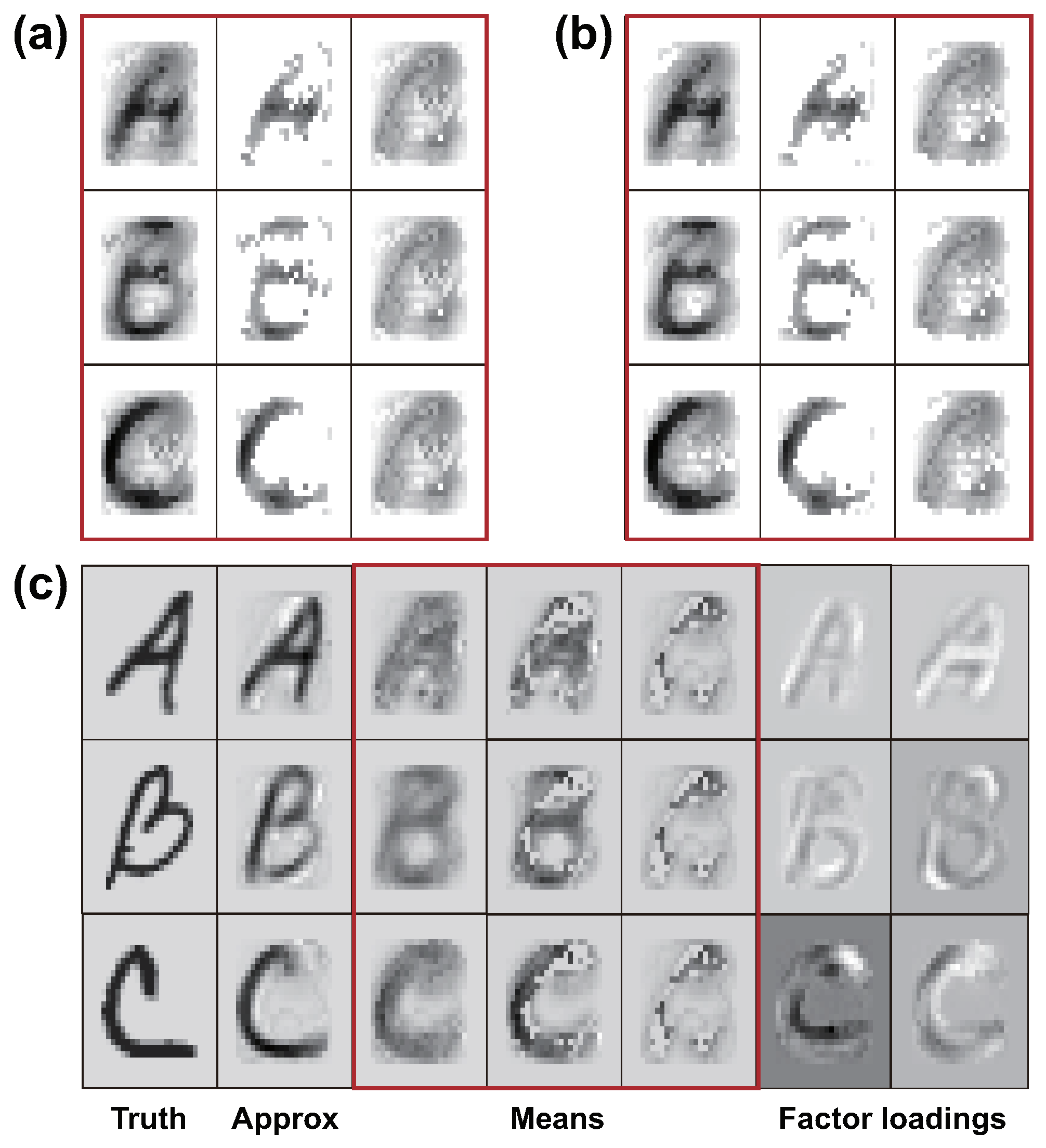
The centroids estimated via the three algorithms are shown in Figure 7, where the reconstruction process of images via the proposed algorithm is also illustrated. The estimated centroid in each class can be calculated following (55), which is a mixing of the class-specific mean and the background. The calculation is outlined by the red box, where the centroid, the class-specific mean and the background are present from left to right, successively. It can be seen that all three algorithms exhibit good performance with respect to characterizing the alphabets. The estimated centroids can sketch the general appearance of the alphabets. But it is noticeable that varFnMS and varFnMS-T make some mistakes on estimation of the background. There should have been no handwritten stroke at the bottom of the background image, since this distinguishes the images of alphabet A. The proposed algorithm performs well with respect to reconstructing the images. An example of reconstruction is present in subplot (c). Additional examples are present in Appendix C. Generally, by adding the influence of latent factors, handwriting on the images becomes legible. The factor loadings on the two most active factors for each alphabet are shown at the right side of subplot (c). As can be seen, the information from latent factors plays an important role in refining the images.
6. Conclusions
In this paper, we developed a hierarchical latent variable model for robust clustering and model selection. We considered the cases where features are correlated within mixture components in a Student’s t mixture model. Factor-adjusted feature saliency was proposed to evaluate the relevance of features to data separation. Automatic latent dimension reduction was achieved by introducing the variables of factor activity. A full Bayesian treatment was adopted and a structured VB inference framework was developed that have enabled a tighter bond to the marginal likelihood and improved the inference accuracy. Controlled experiments on synthetic and real-world datasets showed that the proposed model is able to capture the correlation between features and shows better clustering performance than the models relying on the local independence assumption. Application of the developed algorithm on the high-dimensional handwritten alphabet data showed its applicability and usefulness for image recognition and reconstruction.
In the proposed model, we take the number of clusters (number of components in the mixture model) as fixed and given before inference. An ongoing work is to extend our model to realize automatic selection of the number of clusters. We imposed the Dirichlet prior on the mixing probabilities, which can act as a penalization to drive the mixing probabilities associated with unnecessary components towards extinction. We will also investigate the novel penalization methods proposed in [34] which result in continuous objective functions and can shrink the mixing weights to exactly zero. Other limitations include assuming that features are approximated Gaussian distributed in each component. This assumption can be violated when the features only take positive values or follow skewed distributions. Future work may consider extending the model to tackle these scenarios.
Supplementary Materials
The following supporting information can be downloaded at: https://www.mdpi.com/article/10.3390/math12071091/s1, S1. Deriving the auxiliary posteriors of the latent variables; S2. Deriving the auxiliary posteriors of the parameters.
Author Contributions
Conceptualization, Y.N. and W.X.; methodology, S.F.; software, S.F.; validation, S.F.; formal analysis, S.F.; writing—original draft preparation, S.F.; writing—review and editing, W.X.; visualization, S.F.; supervision, Y.N.; funding acquisition, Y.N. All authors have read and agreed to the published version of the manuscript.
Funding
This research was funded by the National Key R&D Program of China grant number 2020YFA0713603 and the National Natural Science Foundation of China grant number 11971386.
Data Availability Statement
The five datasets used in this study are publicly available. The Iris data can be obtained from the R package “datasets”. (The R software can be downloaded at http://www.r-project.org/; R version is 4.3.1. (accessed on 26 May 2023)) The Olive and Wine data can be obtained from the R package “pgmm”. The Wisconsin diagnostic breast cancer (WDBC) data can be downloaded from the UCI machine learning repository at https://doi.org/10.24432/C5DW2B (accessed on 26 May 2023). The handwritten alphabets data are openly available in the Kaggle webpage: https://www.kaggle.com/datasets/sachinpatel21/az-handwritten-alphabets-in-csv-format/data (accessed on 26 May 2023). The R codes for the developed algorithm are available on request from the authors.
Conflicts of Interest
The authors declare no conflicts of interest.
Appendix A
The evidence lower bound monitoring the optimization process of the proposed algorithm can be evaluated as follows:

Table A1.
Evaluation of the evidence lower bound.
| Expectations of the Logarithm of Priors of the Latent Variables | ||
|---|---|---|
| = | ||
| = | ||
| = | ||
| = | ||
| = | ||
| = | ||
| = | ||
| = | ||
| = | ||
| = | ||
| = | ||
| = | ||
| = | ||
| = | ||
| = | ||
| = | ||
| Expectations of the Logarithm of the Auxiliary Posteriors | ||
| = | ||
| = | ||
| = | ||
| = | ||
| = | ||
| = | ||
| = | ||
| = | ||
| = | ||
| = | ||
| = | ||
| = | ||
| = |
Appendix B
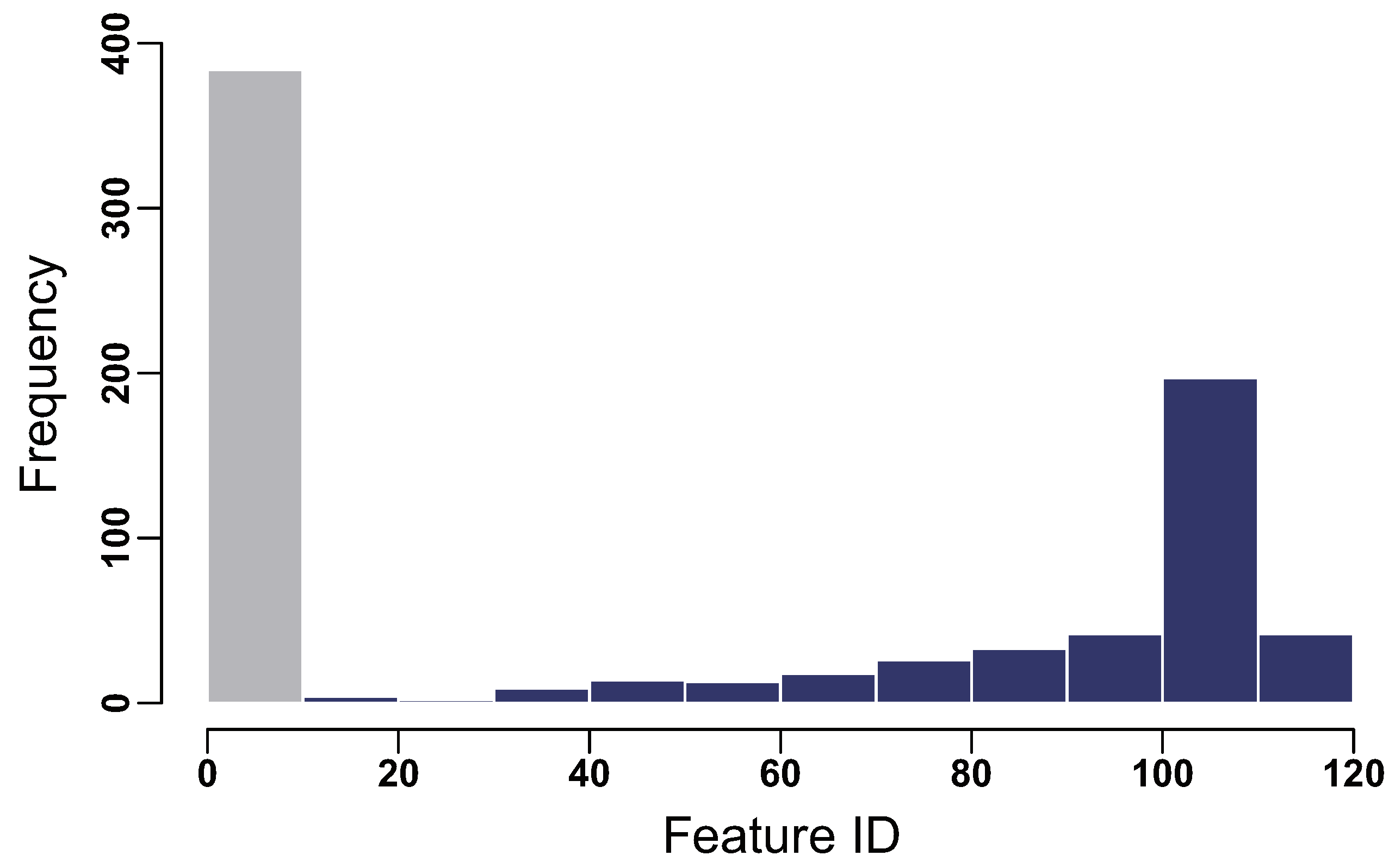
Figure A1 shows the frequency histogram of the standard deviation for features in the handwritten alphabet image. As can be seen, the values of standard deviation range from 0 to 120 and a large proportion of the features have zero variance or comparably small variance. Most of them lie on the marginal area of the image. To improve the computational efficiency, we removed the features with standard deviation smaller than ten at the pre-processing stage which left 400 features for the clustering task.
In addition, we observed the singularity problem during iterations of the clustering algorithms as the variability of some pixels in the image of an alphabet is exactly zero. This happens when the clustering of the images gets close to their original grouping. To tackle the problem, we put a noise mask on the data. Each element of the noise mask was generated from .
Figure A1.
Frequency histogram of the standard deviation for the features in the handwritten alphabet data. The frequency bar corresponding to the standard deviation below 10 is marked in grey.
Figure A1.
Frequency histogram of the standard deviation for the features in the handwritten alphabet data. The frequency bar corresponding to the standard deviation below 10 is marked in grey.

Appendix C
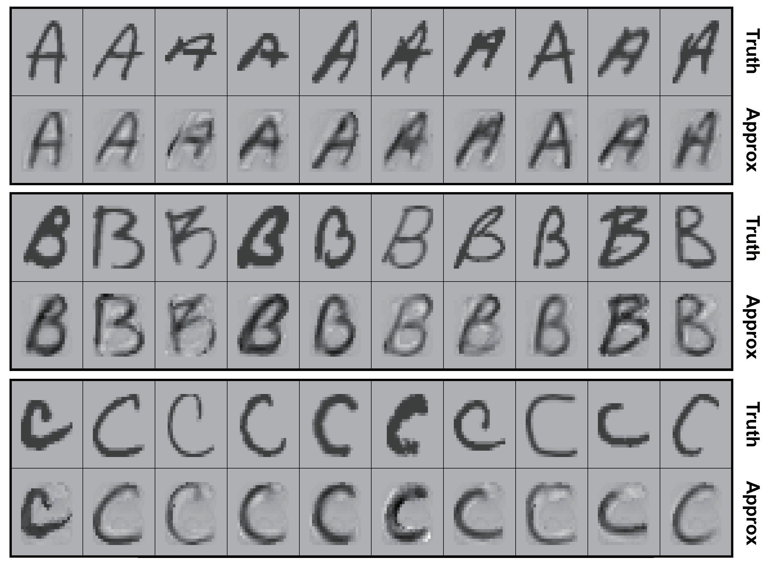
Figure A2 presents the reconstructed images for the alphabet A, B and C by the proposed algorithm.
Figure A2.
Reconstructed images for the handwritten alphabet A, B and C by the proposed algorithm.

References
- Jiang, Z.; Zheng, Y.; Tan, H.; Tang, B.; Zhou, H. Variational deep embedding: An unsupervised and generative approach to clustering. In Proceedings of the 26th International Joint Conference on Artificial Intelligence, Melbourne, Australia, 19–25 August 2017; pp. 1965–1972. [Google Scholar]
- Yang, L.; Cheung, N.M.; Li, J.; Fang, J. Deep clustering by Gaussian mixture variational autoencoders with graph embedding. In Proceedings of the 2019 IEEE/CVF International Conference on Computer Vision (ICCV), Seoul, Republic of Korea, 27 October–2 November 2019; pp. 6440–6449. [Google Scholar]
- Sun, J.; Zhou, A.; Keates, S.; Liao, S. Simultaneous Bayesian clustering and feature selection through student’s t mixtures model. IEEE Trans. Neural Netw. Learn. Syst. 2018, 29, 1187–1199. [Google Scholar] [CrossRef] [PubMed]
- Law, M.H.C.; Figueiredo, M.A.T.; Jain, A.K. Simultaneous feature selection and clustering using mixture models. IEEE Trans. Pattern Anal. Mach. Intell. 2004, 26, 1154–1166. [Google Scholar] [CrossRef] [PubMed]
- Bouveyron, C.; Brunet-Saumard, C. Model-based clustering of high-dimensional data: A review. Comput. Stat. Data Anal. 2014, 71, 52–78. [Google Scholar] [CrossRef]
- Dash, M.; Liu, H. Feature selection for clustering. In Proceedings of the 4th International Conference on the Practical Application of Knowledge Discovery and Data Mining, Crowne Plaza Midland Hotel, Manchester, UK, 11–13 April 2000; Springer: Berlin/Heidelberg, Germany, 2000; pp. 110–121. [Google Scholar]
- Mitra, P.; Murthy, C.; Pal, S. Unsupervised feature selection using feature similarity. IEEE Trans. Pattern Anal. Mach. Intell. 2002, 24, 301–312. [Google Scholar] [CrossRef]
- Pan, W.; Shen, X. Penalized model-based clustering with application to variable selection. J. Mach. Learn. Res. 2007, 8, 1145–1164. [Google Scholar]
- Bhattacharya, S.; McNicholas, P.D. A LASSO-penalized BIC for mixture model selection. Adv. Data Anal. Classif. 2014, 8, 45–61. [Google Scholar] [CrossRef]
- Constantinopoulos, C.; Titsias, M.K.; Likas, A. Bayesian feature and model selection for Gaussian mixture models. IEEE Trans. Pattern Anal. Mach. Intell. 2006, 28, 1013–1018. [Google Scholar] [CrossRef] [PubMed]
- Li, Y.; Dong, M.; Hua, J. Simultaneous localized feature selection and model detection for Gaussian mixtures. IEEE Trans. Pattern Anal. Mach. Intell. 2009, 31, 953–960. [Google Scholar]
- Hong, X.; Li, H.; Miller, P.; Zhou, J.; Li, L.; Crookes, D.; Lu, Y.; Li, X.; Zhou, H. Component-based feature saliency for clustering. IEEE Trans. Knowl. Data Eng. 2021, 33, 882–896. [Google Scholar] [CrossRef]
- Zhang, H.; Wu, Q.M.J.; Nguyen, T.M. Variational Bayes and localized feature selection for student’s t-mixture models. Int. J. Pattern Recognit. Artif. Intell. 2013, 27, 1350016. [Google Scholar] [CrossRef]
- Sun, J.; Zhou, A. Unsupervised robust Bayesian feature selection. In Proceedings of the 2014 International Joint Conference on Neural Networks, Beijing, China, 6–11 July 2014; pp. 558–564. [Google Scholar]
- Perthame, E.; Friguet, C.; Causeur, D. Stability of feature selection in classification issues for high-dimensional correlated data. Stat. Comput. 2016, 26, 783–796. [Google Scholar] [CrossRef]
- Fan, J.; Ke, Y.; Wang, K. Factor-adjusted regularized model selection. J. Econom. 2020, 216, 71–85. [Google Scholar] [CrossRef] [PubMed]
- Mai, Q.; Zou, H.; Yuan, M. A direct approach to sparse discriminant analysis in ultra-high dimensions. Biometrika 2012, 99, 29–42. [Google Scholar] [CrossRef]
- Galimberti, G.; Soffritti, G. Using conditional independence for parsimonious model-based Gaussian clustering. Stat. Comput. 2013, 23, 625–638. [Google Scholar] [CrossRef]
- Devijver, E.; Gallopin, M. Block-diagonal covariance selection for high-dimensional Gaussian graphical models. J. Am. Stat. Assoc. 2018, 113, 306–314. [Google Scholar] [CrossRef]
- Ruan, L.; Yuan, M.; Zou, H. Regularized parameter estimation in high-dimensional Gaussian mixture models. Neural Comput. 2011, 23, 1605–1622. [Google Scholar] [CrossRef] [PubMed]
- McLachlan, G.J.; Bean, R.W.; Jones, L.B.T. Extension of the mixture of factor analyzers model to incorporate the multivariate t-distribution. Comput. Stat. Data Anal. 2007, 51, 5327–5338. [Google Scholar] [CrossRef]
- Archambeau, C.; Delannay, N.; Verleysen, M. Mixtures of robust probabilistic principal component analyzers. Neurocomputing 2008, 71, 1274–1282. [Google Scholar] [CrossRef]
- McNicholas, P.D.; Murphy, T.B. Model-based clustering of microarray expression data via latent Gaussian mixture models. Bioinformatics 2010, 26, 2705–2712. [Google Scholar] [CrossRef]
- Andrews, J.L.; McNicholas, P.D. Extending mixtures of multivariate t-factor analyzers. Stat. Comput. 2011, 21, 361–373. [Google Scholar] [CrossRef]
- Wang, Z.; Lan, C. Towards a hierarchical Bayesian model of multi-view anomaly detection. In Proceedings of the 29th International Joint Conference on Artificial Intelligence, Yokohama, Japan, 7–15 January 2020; pp. 2420–2426. [Google Scholar]
- Mackay, D.J.C. Probable networks and plausible predictions—A review of practical Bayesian methods for supervised neural networks. Netw. Comput. Neural Syst. 1995, 6, 469–505. [Google Scholar] [CrossRef]
- Bhattacharya, A.; Dunson, D.B. Sparse Bayesian infinite factor models. Biometrika 2011, 98, 291–306. [Google Scholar] [CrossRef] [PubMed]
- Murphy, K.; Viroli, C.; Gormley, I.C. Infinite mixtures of infinite factor analysers. Bayesian Anal. 2020, 15, 937–963. [Google Scholar] [CrossRef]
- Ormerod, J.T.; You, C.; Müller, S. A variational Bayes approach to variable selection. Electron. J. Stat. 2017, 11, 3549–3594. [Google Scholar] [CrossRef]
- Gal, Y.; Ghahramani, Z. Dropout as a Bayesian approximation: Representing model uncertainty in deep learning. In Proceedings of the 33rd International Conference on International Conference on Machine Learning, New York, NY, USA, 19–24 June 2016; Volume 48, pp. 1050–1059. [Google Scholar]
- Beal, M.J.; Ghahramani, Z. The variational Bayesian EM algorithm for incomplete data: With application to scoring graphical model structures. In Bayesian Statistic 7: Proceedings of the Seventh Valencia International Meeting; Oxford University Press: Oxford, UK, 2003; pp. 453–463. [Google Scholar]
- Teh, Y.W.; Newman, D.; Welling, M. A collapsed variational Bayesian inference algorithm for latent Dirichlet allocation. In Advances in Neural Information Processing Systems 19 Proceedings of the 2006 Conference; MIT Press: Cambridge, MA, USA, 2006; pp. 1353–1360. [Google Scholar]
- Zhang, C.X.; Xu, S.; Zhang, J.S. A novel variational Bayesian method for variable selection in logistic regression models. Comput. Stat. Data Anal. 2019, 133, 1–19. [Google Scholar] [CrossRef]
- Huang, T.; Peng, H.; Zhang, K. Model selection for Gaussian mixture models. Stat. Sin. 2017, 27, 147–169. [Google Scholar] [CrossRef]
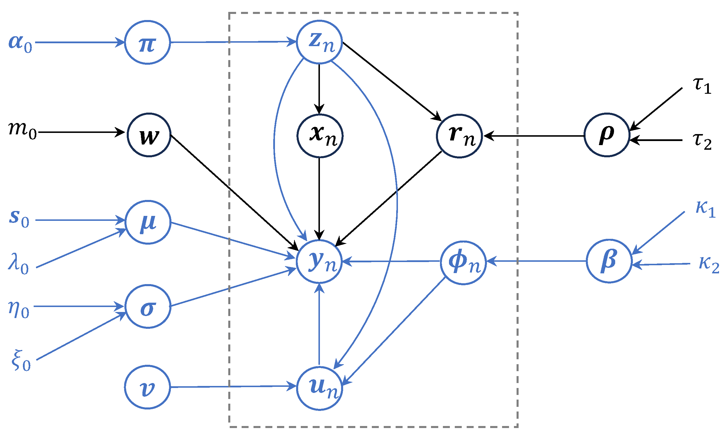
Figure 1.
Plate diagram of the proposed hierarchical latent variable model.

Figure 2.
Factor activity estimated by the proposed algorithm for the two synthetic datasets where the features are locally (a) independent and (b) correlated, separately.
Figure 2.
Factor activity estimated by the proposed algorithm for the two synthetic datasets where the features are locally (a) independent and (b) correlated, separately.

Figure 3.
Feature saliency estimated via varFnMS (left), varFnMS-T (middle) and varFnMS-TFA (right) for the two synthetic datasets where the features are locally (a) independent and (b) correlated, separately.
Figure 3.
Feature saliency estimated via varFnMS (left), varFnMS-T (middle) and varFnMS-TFA (right) for the two synthetic datasets where the features are locally (a) independent and (b) correlated, separately.

Figure 4.
Factor activity estimated via the proposed algorithm for the four benchmark datasets: (a) Iris, (b) Olive, (c) Wine and (d) WDBC.
Figure 4.
Factor activity estimated via the proposed algorithm for the four benchmark datasets: (a) Iris, (b) Olive, (c) Wine and (d) WDBC.

Figure 5.
Feature saliency estimated via varFnMS (left), varFnMS-T (middle) and varFnMS-TFA (right) for the four benchmark datasets: (a) Iris, (b) Olive, (c) Wine and (d) WDBC. The saliency level at 0.5 is marked by the red dotted line.
Figure 5.
Feature saliency estimated via varFnMS (left), varFnMS-T (middle) and varFnMS-TFA (right) for the four benchmark datasets: (a) Iris, (b) Olive, (c) Wine and (d) WDBC. The saliency level at 0.5 is marked by the red dotted line.

Figure 6.
Feature saliency estimated via varFnMS (left), varFnMS-T (middle) and varFnMS-TFA (right) for the handwritten alphabet data. The saliency level at 0.5 is marked by the red dotted line.
Figure 6.
Feature saliency estimated via varFnMS (left), varFnMS-T (middle) and varFnMS-TFA (right) for the handwritten alphabet data. The saliency level at 0.5 is marked by the red dotted line.

Figure 7.
Reconstruction of the handwritten alphabet image via varFnMS (a), varFnMS-T (b) and varFnMS-TFA (c). The estimated centroids are outlined with a red box, where the centroid, the class-specific mean and the background are present from left to right, successively.
Figure 7.
Reconstruction of the handwritten alphabet image via varFnMS (a), varFnMS-T (b) and varFnMS-TFA (c). The estimated centroids are outlined with a red box, where the centroid, the class-specific mean and the background are present from left to right, successively.

Table 1.
Evidence lower bound (ELBO) and classification error obtained via varFnMS, varFnMS-T and varFnMS-TFA for the two synthetic datasets where the features are locally independent and correlated, separately.
Table 1.
Evidence lower bound (ELBO) and classification error obtained via varFnMS, varFnMS-T and varFnMS-TFA for the two synthetic datasets where the features are locally independent and correlated, separately.
| Independent | Correlated | |||
|---|---|---|---|---|
| Algorithm | ELBO | Error | ELBO | Error |
| varFnMS | −13,320.803 | 0.076 | −16,868.400 | 0.351 |
| (136.822) | (0.118) | (113.338) | (0.071) | |
| varFnMS-T | −13,140.178 | 0.073 | −16,468.433 | 0.302 |
| (763.027) | (0.111) | (135.973) | (0.083) | |
| varFnMS-TFA | −9082.876 | 0.071 | −8854.751 | 0.051 |
| (3320.315) | (0.109) | (2696.577) | (0.053) | |
Table 2.
The centroids estimated via varFnMS, varFnMS-T and varFnMS-TFA for the two synthetic datasets where the features are locally independent and correlated, separately.
Table 2.
The centroids estimated via varFnMS, varFnMS-T and varFnMS-TFA for the two synthetic datasets where the features are locally independent and correlated, separately.
| Independent | Correlated | |||||
|---|---|---|---|---|---|---|
| Class 1 | varFnMS | varFnMS-T | varFnMS-TFA | varFnMS | varFnMS-T | varFnMS-TFA |
| 0.405 (0.791) | 0.399 (0.910) | 0.392 (0.906) | 0.739 (1.056) | 0.064 (0.569) | 0.019 (0.140) | |
| 3.289 (0.664) | 3.178 (0.471) | 3.223 (0.670) | 3.922 (1.405) | 1.771 (1.270) | 3.093 (0.201) | |
| 0.000 (0.037) | −0.107 (0.497) | −0.116 (0.490) | −0.314 (0.760) | −1.730 (0.952) | −0.001 (0.121) | |
| −0.007 (0.049) | 0.041 (0.178) | −0.027 (0.096) | −0.009 (0.776) | −1.053 (0.814) | −0.025 (0.078) | |
| 0.002 (0.043) | −0.025 (0.098) | 0.000 (0.044) | −0.271 (0.915) | −1.748 (0.869) | −0.020 (0.041) | |
| 0.005 (0.044) | −0.086 (0.393) | −0.031 (0.121) | 0.011 (0.210) | −0.390 (0.428) | 0.000 (0.000) | |
| −0.016 (0.043) | −0.073 (0.292) | −0.017 (0.046) | −0.185 (0.543) | 0.060 (0.537) | −0.014 (0.046) | |
| −0.007 (0.039) | −0.051 (0.194) | −0.032 (0.119) | −0.004 (0.448) | 0.340 (0.670) | −0.052 (0.180) | |
| 0.034 (0.050) | 0.075 (0.228) | 0.015 (0.032) | 0.019 (0.866) | 1.410 (0.979) | −0.012 (0.028) | |
| −0.021 (0.040) | −0.168 (0.662) | −0.034 (0.125) | 0.026 (0.422) | 0.262 (0.237) | −0.004 (0.030) | |
| Class 2 | varFnMS | varFnMS-T | varFnMS-TFA | varFnMS | varFnMS-T | varFnMS-TFA |
| 1.332 (0.650) | 1.096 (0.447) | 1.058 (0.282) | 2.000 (0.939) | 1.129 (0.678) | 1.049 (0.151) | |
| 8.798 (0.802) | 8.875 (0.478) | 8.793 (0.862) | 6.712 (1.229) | 6.762 (0.863) | 9.012 (0.101) | |
| 0.100 (0.472) | 0.136 (0.622) | 0.040 (0.209) | −0.024 (0.984) | 0.340 (0.315) | 0.008 (0.066) | |
| 0.002 (0.057) | 0.015 (0.047) | 0.008 (0.035) | 0.071 (0.738) | 0.487 (0.792) | 0.042 (0.091) | |
| −0.207 (0.926) | −0.228 (1.006) | −0.192 (0.865) | −0.028 (0.647) | 0.394 (0.321) | −0.011 (0.028) | |
| −0.049 (0.138) | −0.049 (0.167) | −0.012 (0.037) | −0.107 (0.566) | 0.124 (0.305) | 0.004 (0.019) | |
| −0.034 (0.200) | −0.053 (0.231) | −0.001 (0.027) | −0.293 (0.578) | −0.468 (0.615) | −0.007 (0.031) | |
| −0.083 (0.367) | −0.094 (0.423) | −0.093 (0.417) | −0.052 (0.684) | −0.213 (0.314) | 0.008 (0.067) | |
| 0.036 (0.189) | 0.039 (0.202) | 0.004 (0.033) | −0.340 (0.611) | −0.702 (0.637) | −0.009 (0.027) | |
| 0.009 (0.129) | 0.018 (0.193) | 0.040 (0.245) | −0.099 (0.550) | −0.147 (0.160) | 0.002 (0.032) | |
| Class 3 | ||||||
| 5.684 (1.136) | 5.691 (0.998) | 5.758 (0.767) | 4.773 (1.507) | 5.313 (1.603) | 6.013 (0.158) | |
| 4.392 (0.843) | 4.514 (1.246) | 4.553 (1.464) | 3.962 (0.782) | 3.644 (0.726) | 4.174 (0.656) | |
| −0.082 (0.504) | 0.056 (0.402) | 0.064 (0.215) | 0.206 (0.502) | 0.127 (0.454) | 0.018 (0.049) | |
| 0.114 (0.570) | −0.015 (0.722) | −0.063 (0.631) | 0.053 (0.466) | −0.204 (0.516) | 0.006 (0.037) | |
| −0.025 (0.289) | −0.015 (0.330) | 0.062 (0.305) | 0.197 (0.517) | 0.131 (0.428) | −0.011 (0.019) | |
| −0.181 (0.557) | −0.032 (0.632) | −0.087 (0.854) | 0.076 (0.390) | 0.064 (0.196) | 0.002 (0.008) | |
| −0.137 (0.646) | −0.176 (0.761) | −0.213 (0.649) | 0.269 (0.495) | 0.703 (0.619) | −0.005 (0.051) | |
| −0.241 (0.744) | −0.332 (0.946) | −0.141 (0.465) | −0.170 (0.599) | 0.216 (0.427) | 0.010 (0.034) | |
| 0.030 (0.270) | −0.030 (0.196) | −0.017 (0.158) | −0.023 (0.711) | 0.468 (0.629) | −0.012 (0.033) | |
| −0.309 (0.771) | −0.304 (0.767) | −0.142 (0.416) | −0.017 (0.512) | 0.068 (0.156) | −0.001 (0.030) | |
| Class 4 | ||||||
| 6.792 (0.752) | 6.966 (0.130) | 6.960 (0.123) | 5.443 (1.236) | 6.329 (0.899) | 6.709 (1.289) | |
| 9.857 (0.521) | 9.830 (0.689) | 9.831 (0.688) | 9.039 (1.183) | 9.649 (0.623) | 9.741 (0.995) | |
| 0.002 (0.051) | −0.007 (0.060) | −0.005 (0.045) | 0.075 (0.100) | 0.034 (0.079) | −0.006 (0.046) | |
| 0.000 (0.053) | 0.005 (0.036) | 0.000 (0.021) | −0.072 (0.111) | −0.061 (0.129) | 0.380 (1.725) | |
| 0.008 (0.043) | 0.009 (0.041) | 0.002 (0.032) | 0.043 (0.175) | −0.013 (0.096) | −0.015 (0.027) | |
| −0.003 (0.041) | −0.003 (0.037) | −0.006 (0.025) | −0.017 (0.095) | −0.044 (0.084) | 0.002 (0.008) | |
| −0.025 (0.063) | −0.011 (0.058) | 0.002 (0.026) | 0.111 (0.117) | 0.079 (0.098) | −0.097 (0.425) | |
| −0.003 (0.051) | −0.005 (0.045) | −0.004 (0.031) | −0.053 (0.106) | −0.026 (0.077) | 0.081 (0.434) | |
| 0.029 (0.055) | 0.021 (0.051) | 0.016 (0.032) | 0.071 (0.118) | 0.050 (0.106) | −0.011 (0.035) | |
| −0.026 (0.048) | −0.027 (0.049) | −0.011 (0.036) | −0.001 (0.059) | 0.015 (0.053) | −0.001 (0.031) | |
Table 3.
Classification error obtained via varFnMS, varFnMS-T and varFnMFAS-T for the four benchmark datasets.
Table 3.
Classification error obtained via varFnMS, varFnMS-T and varFnMFAS-T for the four benchmark datasets.
| Dataset | N | d | K | varFnMS | varFnMS-T | varFnMS-TFA |
|---|---|---|---|---|---|---|
| Iris | 150 | 4 | 3 | 0.093 | 0.093 | 0.020 |
| Olive | 572 | 8 | 3 | 0.203 | 0.199 | 0.042 |
| Wine | 178 | 27 | 3 | 0.079 | 0.062 | 0.073 |
| WDBC | 569 | 30 | 2 | 0.095 | 0.095 | 0.088 |
Disclaimer/Publisher’s Note: The statements, opinions and data contained in all publications are solely those of the individual author(s) and contributor(s) and not of MDPI and/or the editor(s). MDPI and/or the editor(s) disclaim responsibility for any injury to people or property resulting from any ideas, methods, instructions or products referred to in the content. |
© 2024 by the authors. Licensee MDPI, Basel, Switzerland. This article is an open access article distributed under the terms and conditions of the Creative Commons Attribution (CC BY) license (https://creativecommons.org/licenses/by/4.0/).
Share and Cite
MDPI and ACS Style
Feng, S.; Xie, W.; Nie, Y. Simultaneous Bayesian Clustering and Model Selection with Mixture of Robust Factor Analyzers. Mathematics 2024, 12, 1091. https://doi.org/10.3390/math12071091
AMA Style
Feng S, Xie W, Nie Y. Simultaneous Bayesian Clustering and Model Selection with Mixture of Robust Factor Analyzers. Mathematics. 2024; 12(7):1091. https://doi.org/10.3390/math12071091
Chicago/Turabian StyleFeng, Shan, Wenxian Xie, and Yufeng Nie. 2024. "Simultaneous Bayesian Clustering and Model Selection with Mixture of Robust Factor Analyzers" Mathematics 12, no. 7: 1091. https://doi.org/10.3390/math12071091
Note that from the first issue of 2016, this journal uses article numbers instead of page numbers. See further details here.