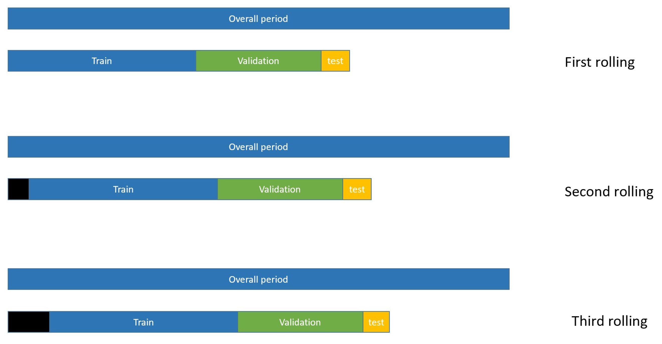
Figure 1.
Split data into training period, validation period, and test period on a rolling basis. For each rolling (colored bars), one BTPB is fit on the training period, and the validation period is used for hyperparameter tuning. Black bars indicate the historical period that is not included in the current windows.
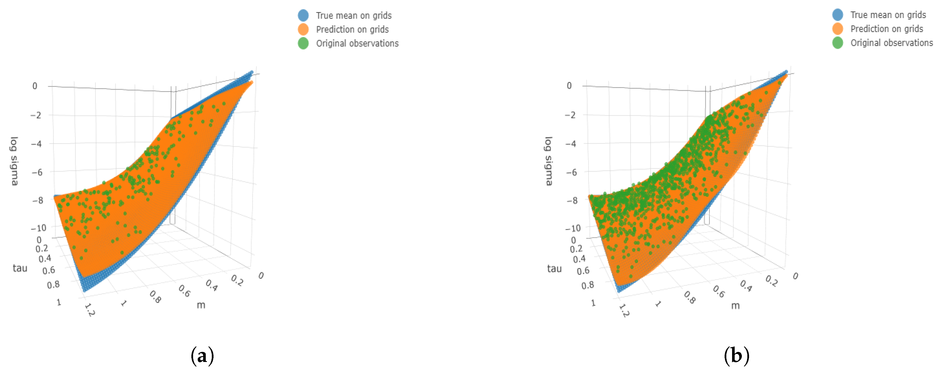
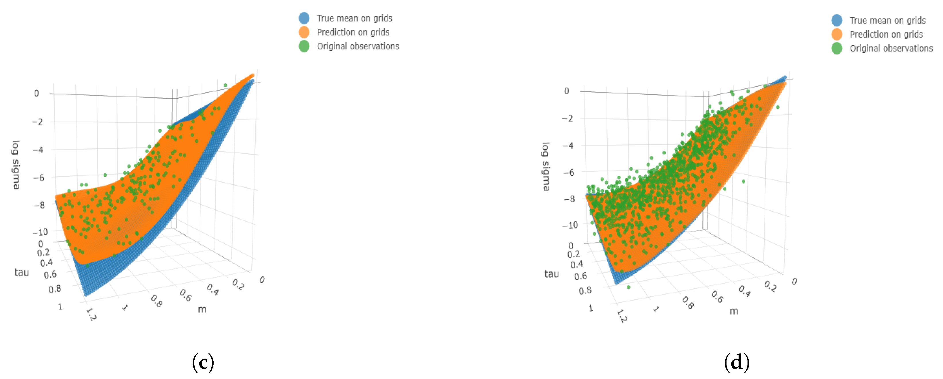
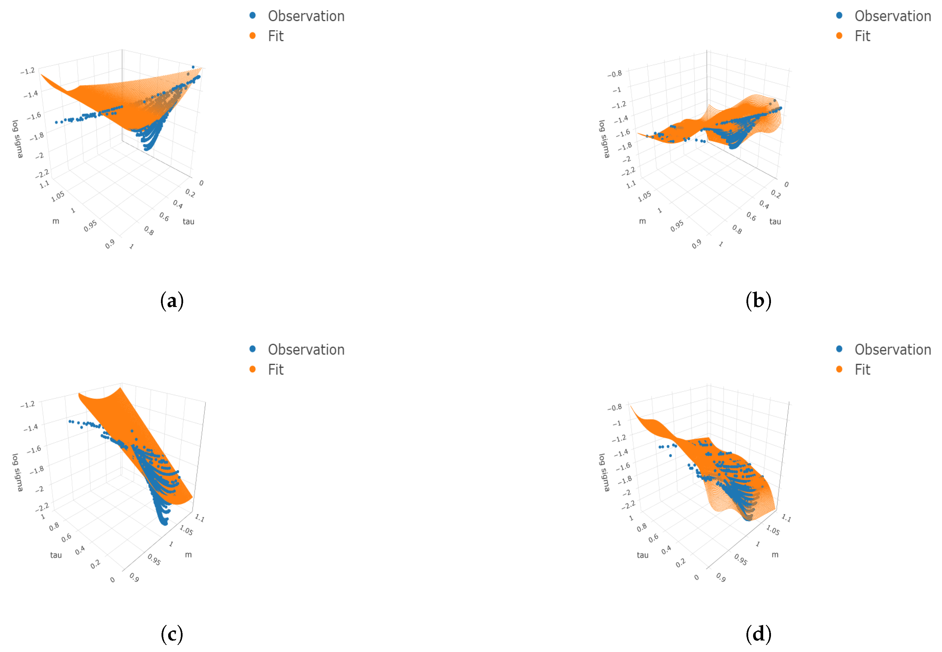
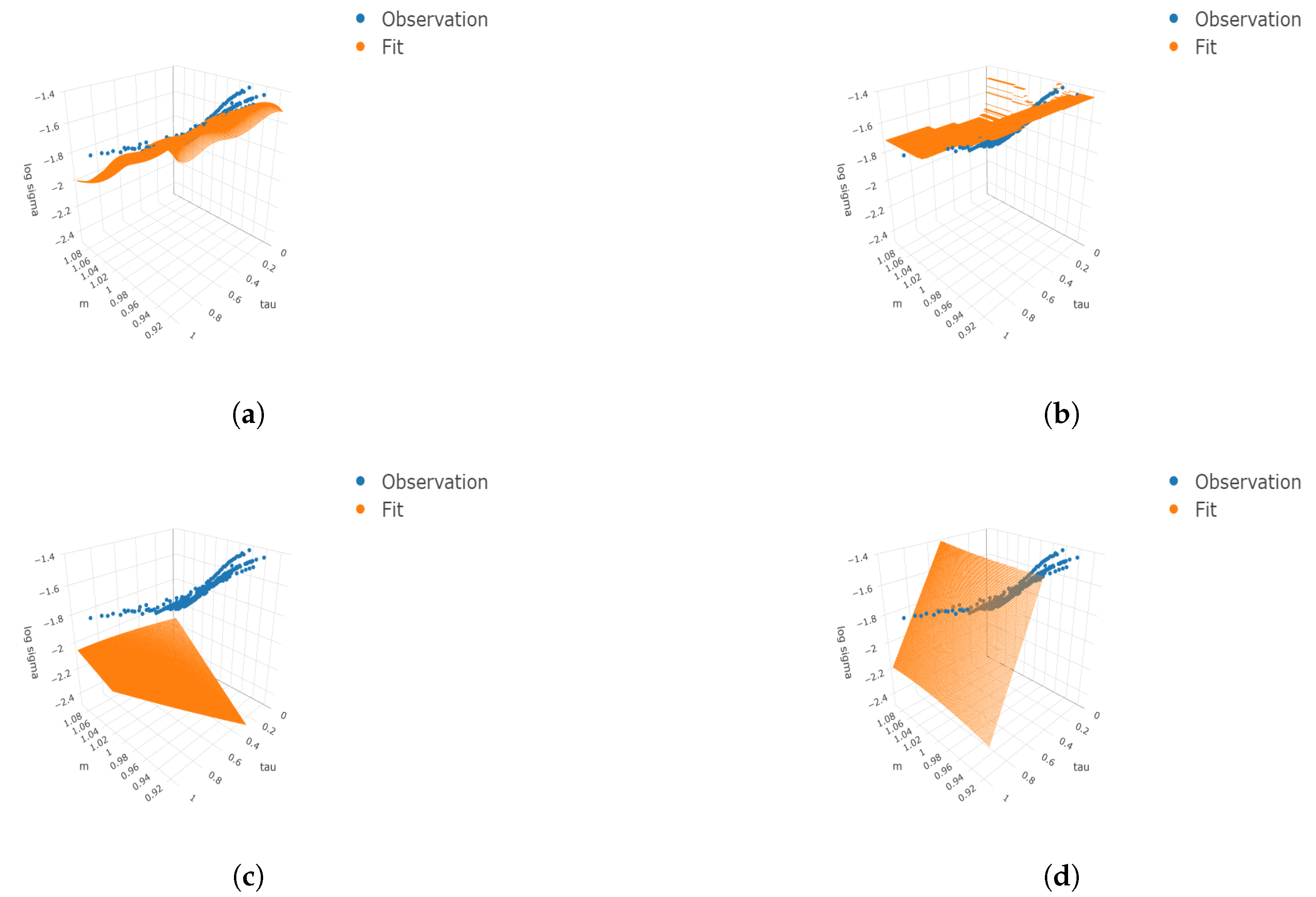
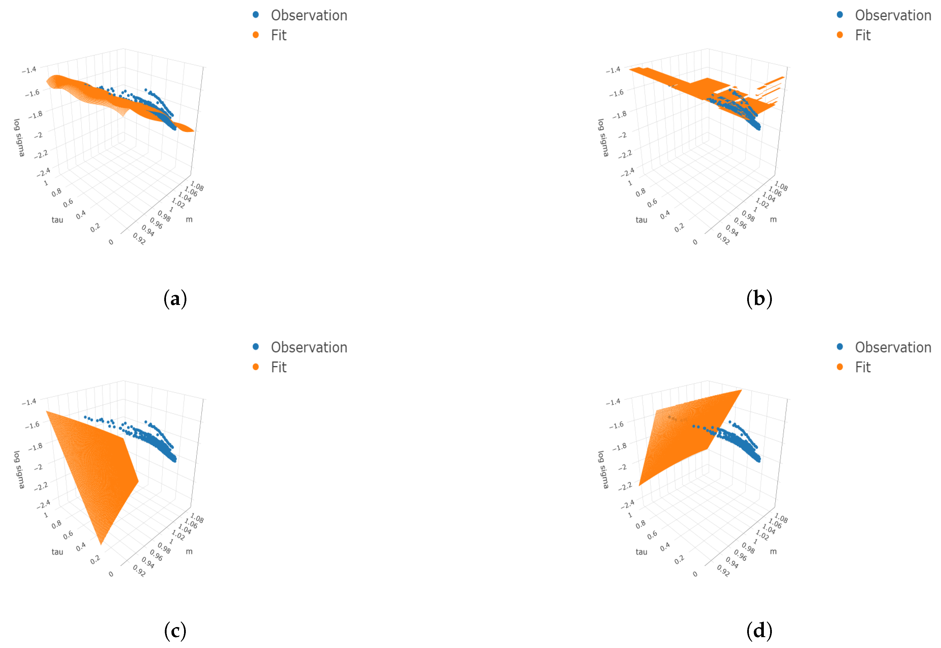
Figure 2.
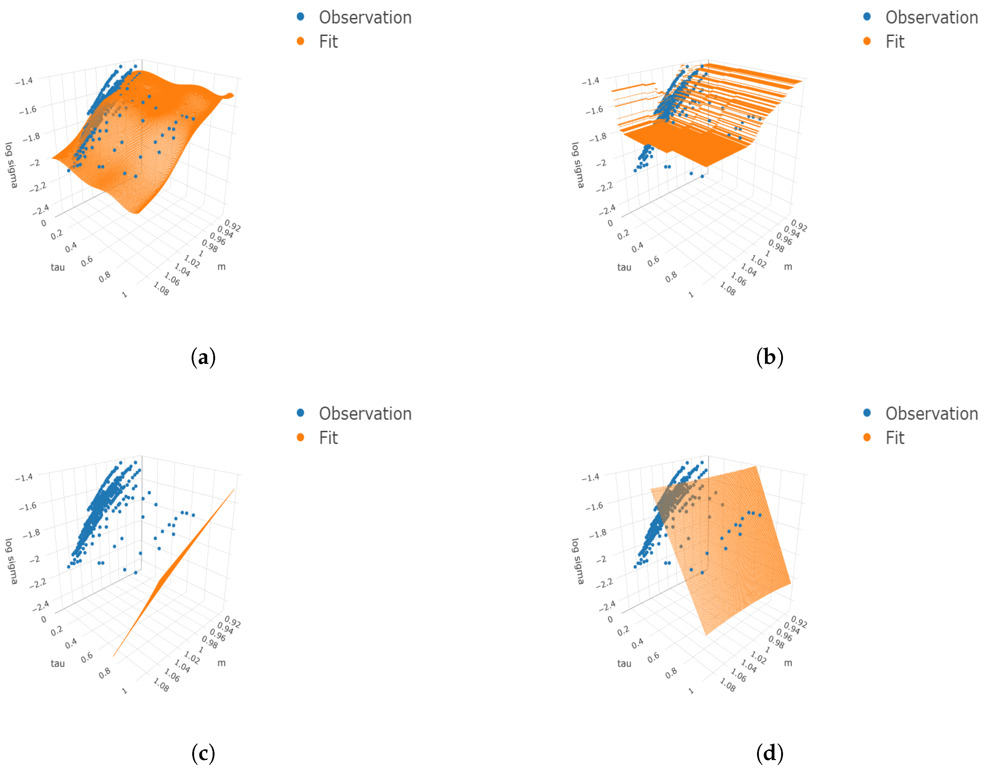
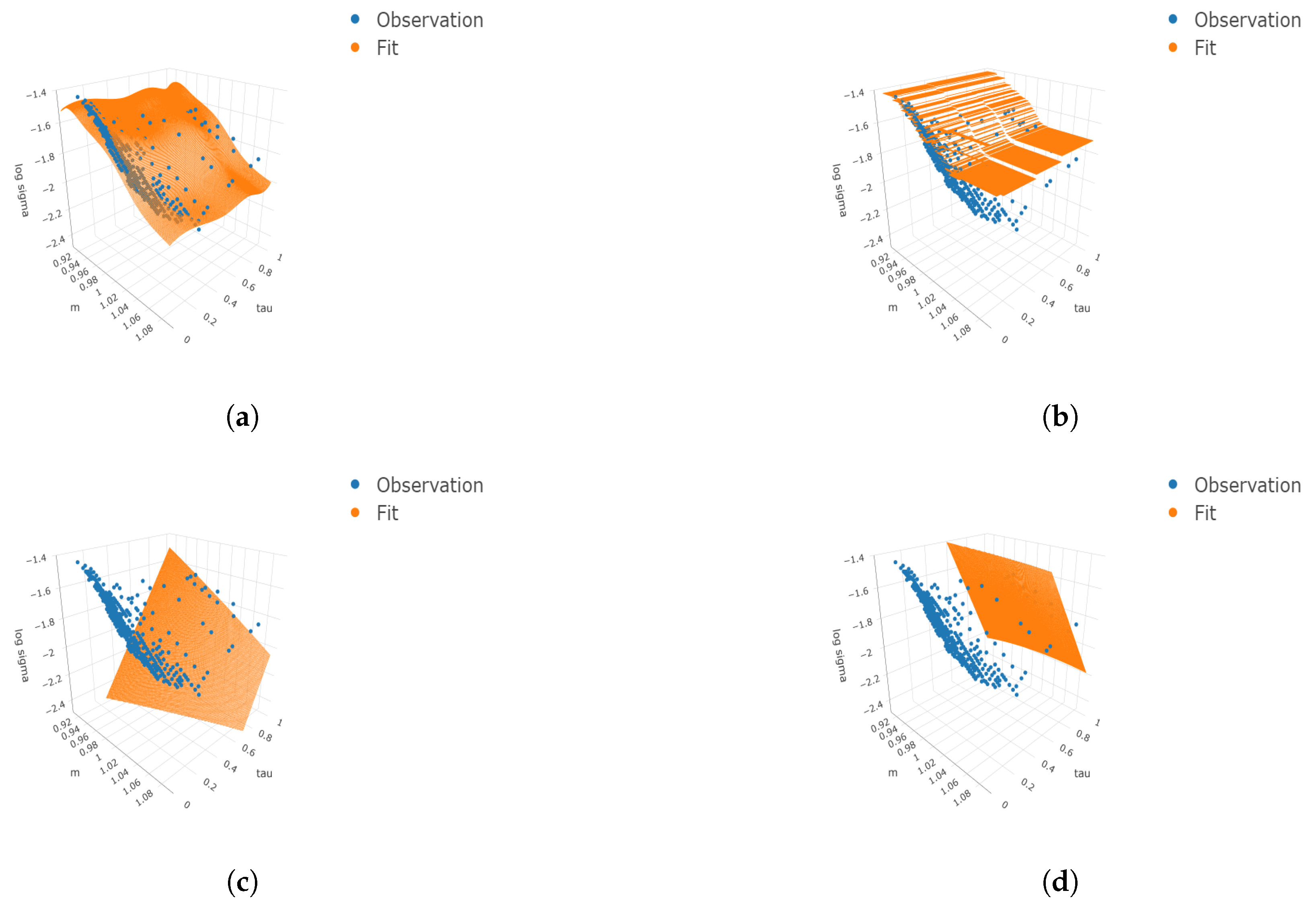
Three-dimensional surface plots under four cases. We consider the finer grids 100 and 50 for and respectively. The true means, simulated observations, and predicted values are plotted on the finer grids as well as the simulated observations. (a) ; (b) ; (c) ; (d) .
Figure 2.
Three-dimensional surface plots under four cases. We consider the finer grids 100 and 50 for and respectively. The true means, simulated observations, and predicted values are plotted on the finer grids as well as the simulated observations. (a) ; (b) ; (c) ; (d) .
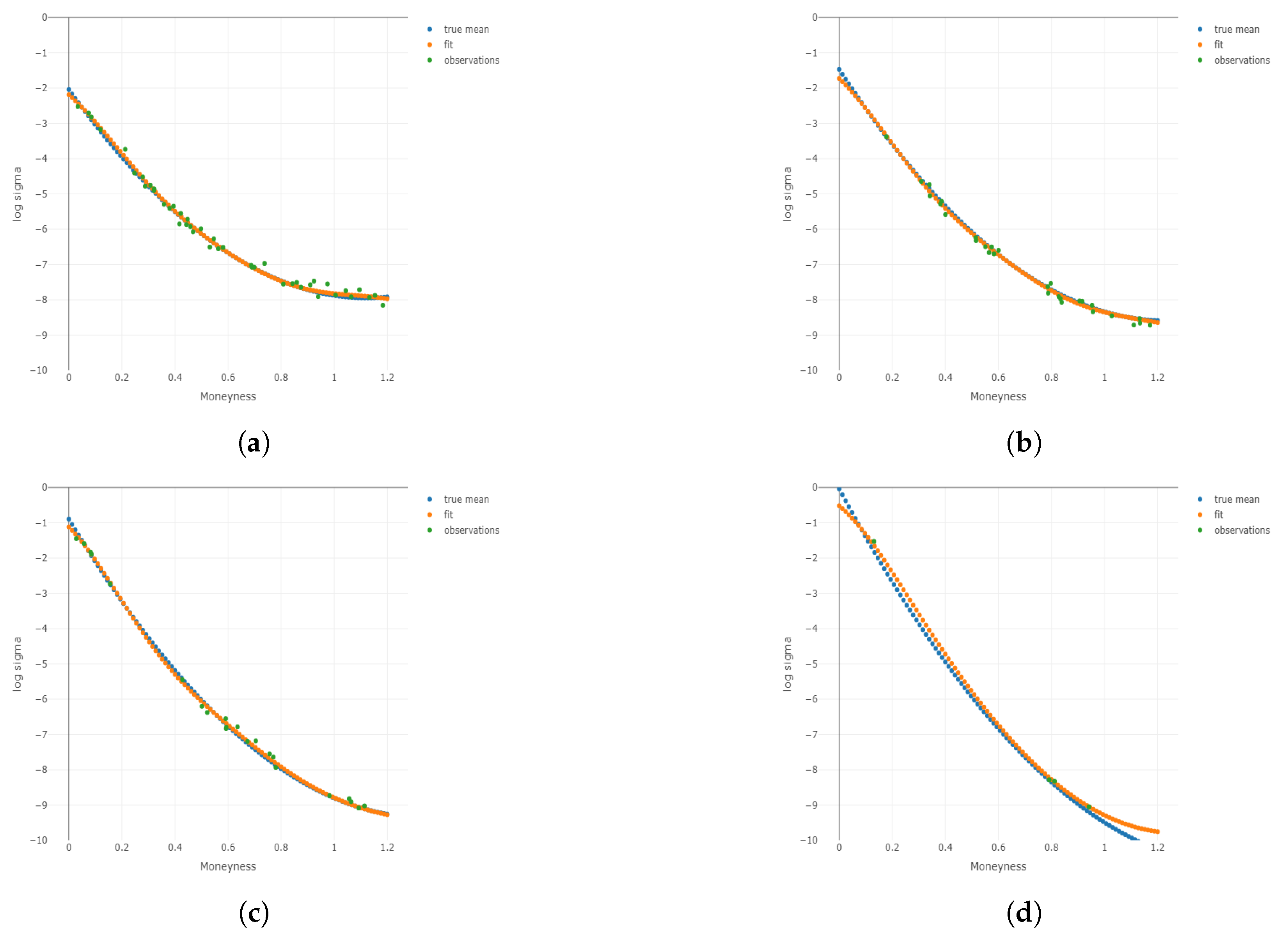
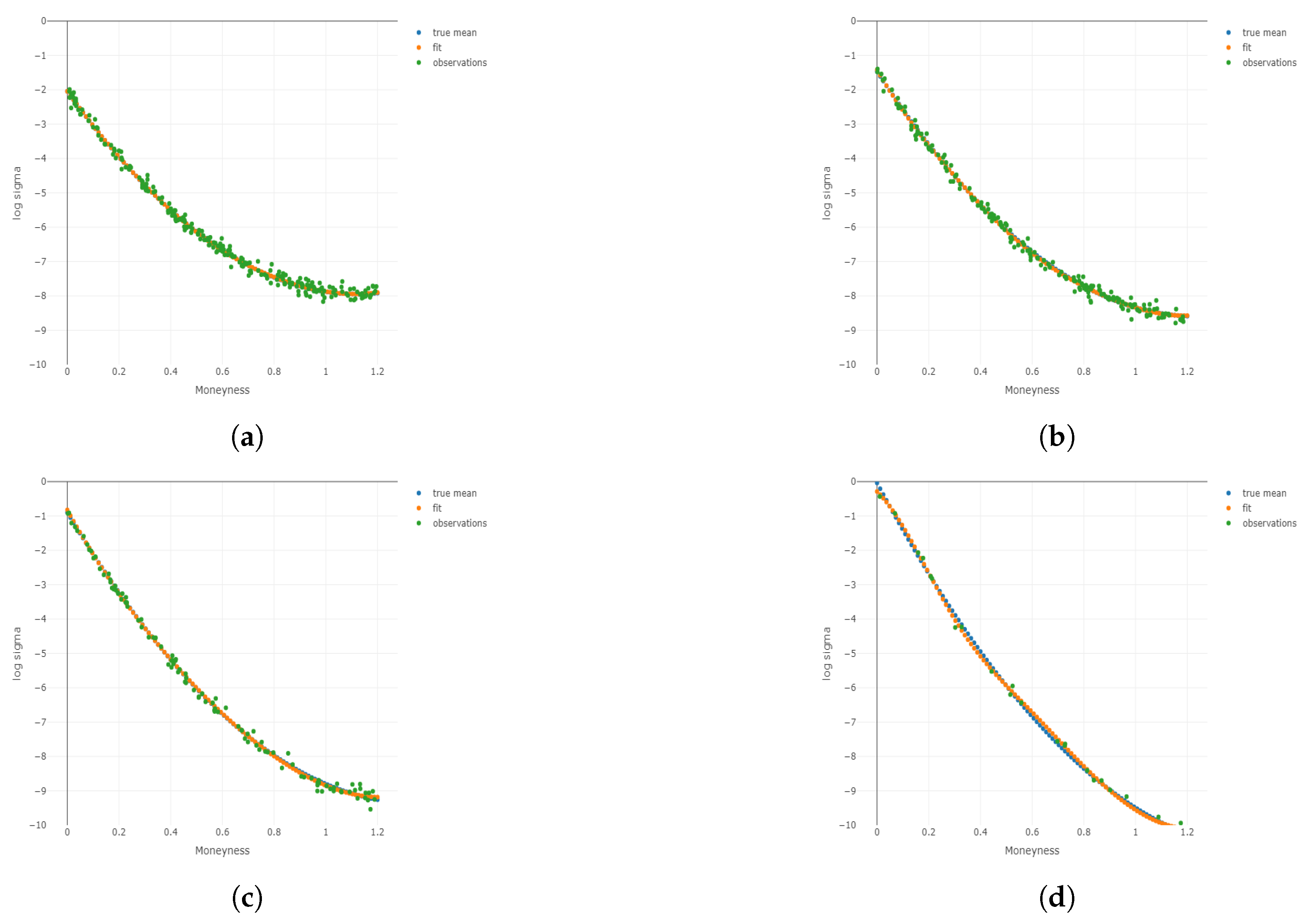
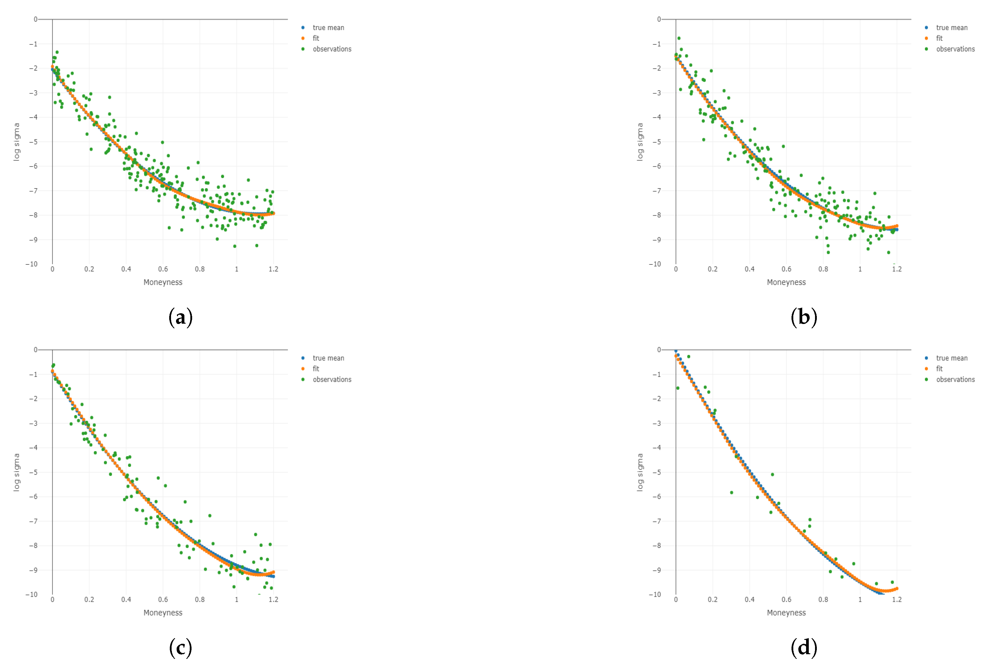
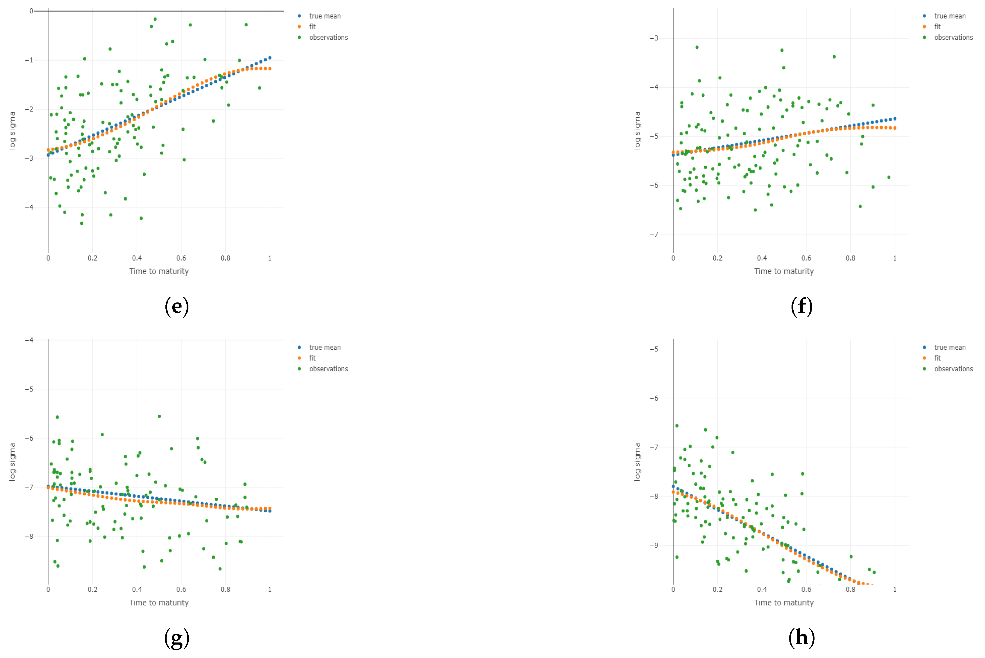
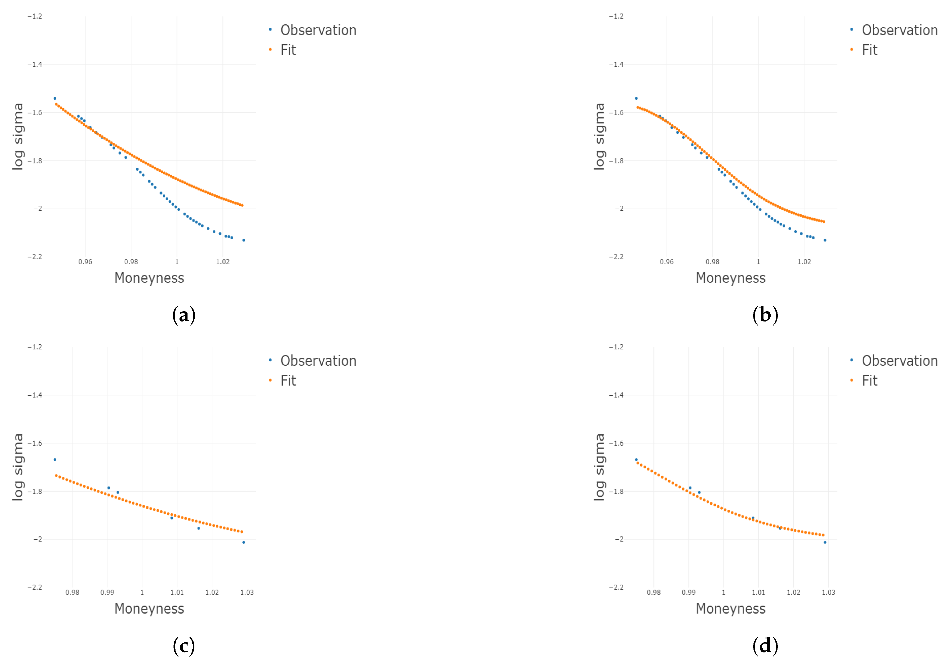
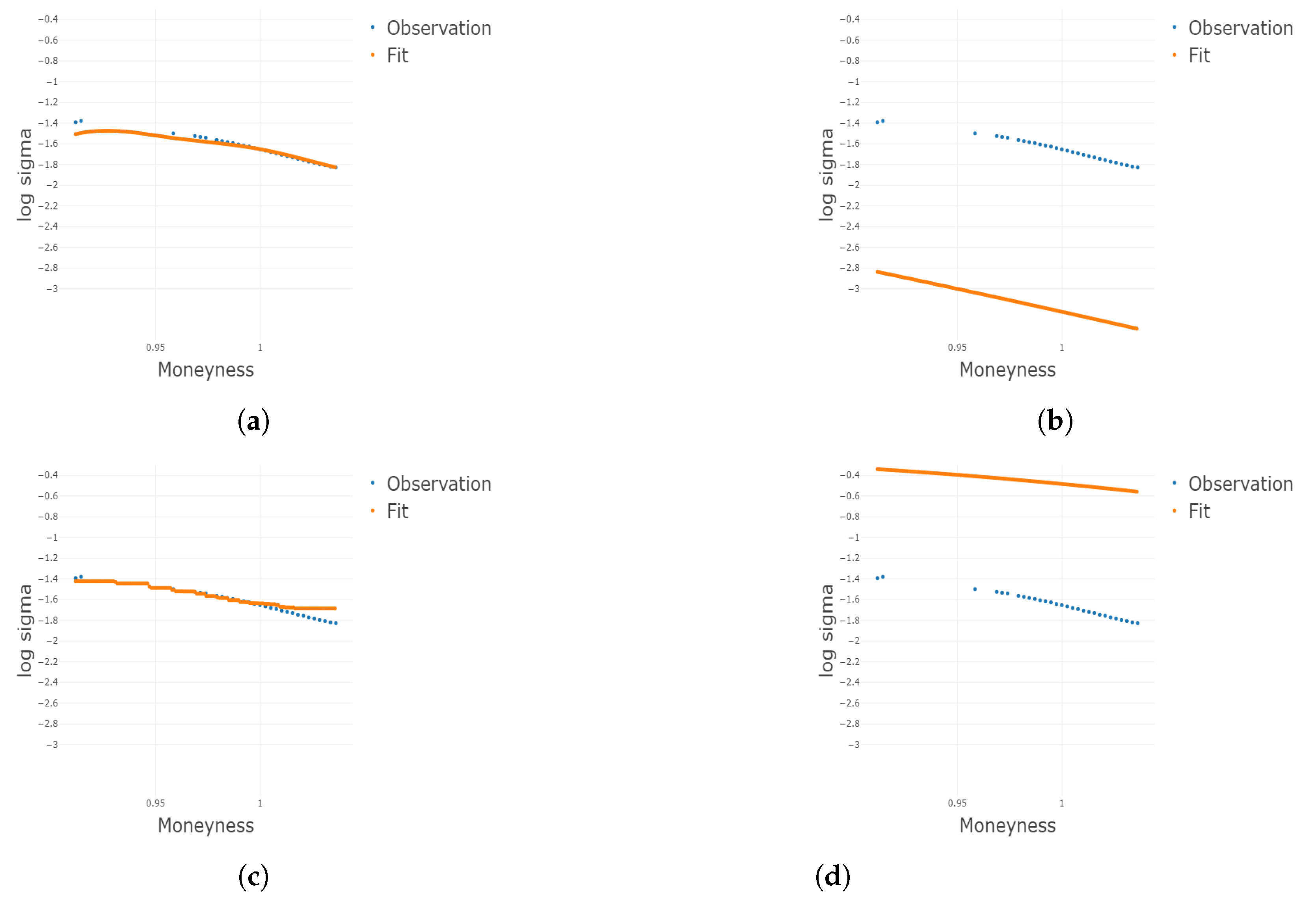
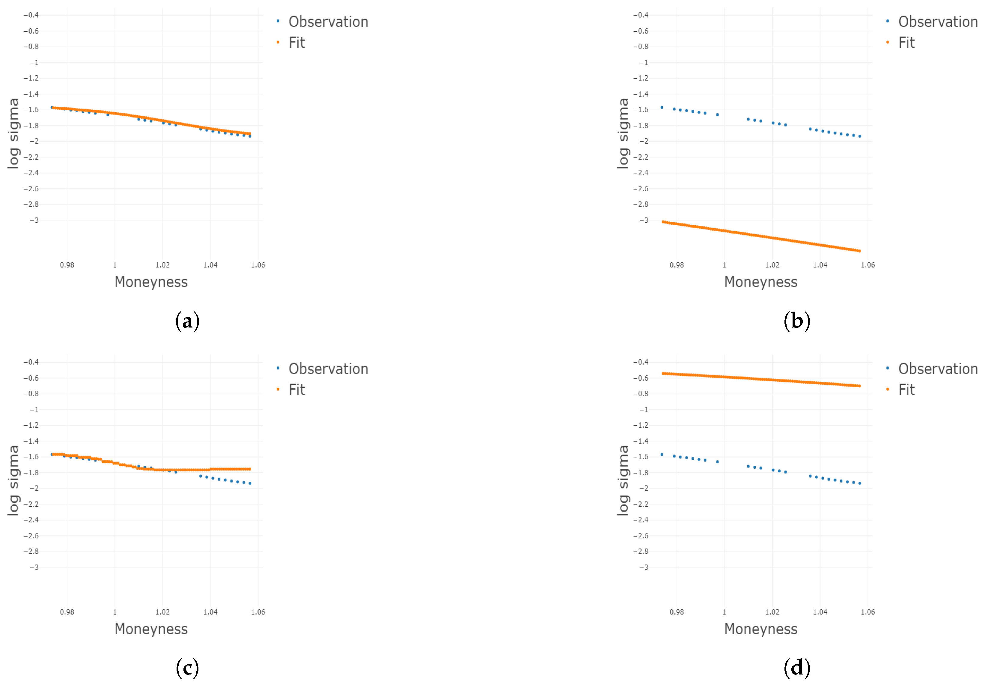
Figure 3.
Two-dimensional plots for different conditional on different and m under . Plots for the 1st, 3rd, 5th, and 8th group are shown conditional on and m, respectively. (a) Two-dimensional plots conditional on the center of the 1st group of ; (b) 2D plots conditional on the center of the 3rd group of ; (c) 2D plots conditional on the center of the 5th group of ; (d) 2D plots conditional on the center of the 8th group of ; (e) 2D plots conditional on the center of the 1st group of m; (f) 2D plots conditional on the center of the 3rd group of m; (g) 2D plots conditional on the center of the 5th group of m; (h) 2D plots conditional on the center of the 8th group of m.
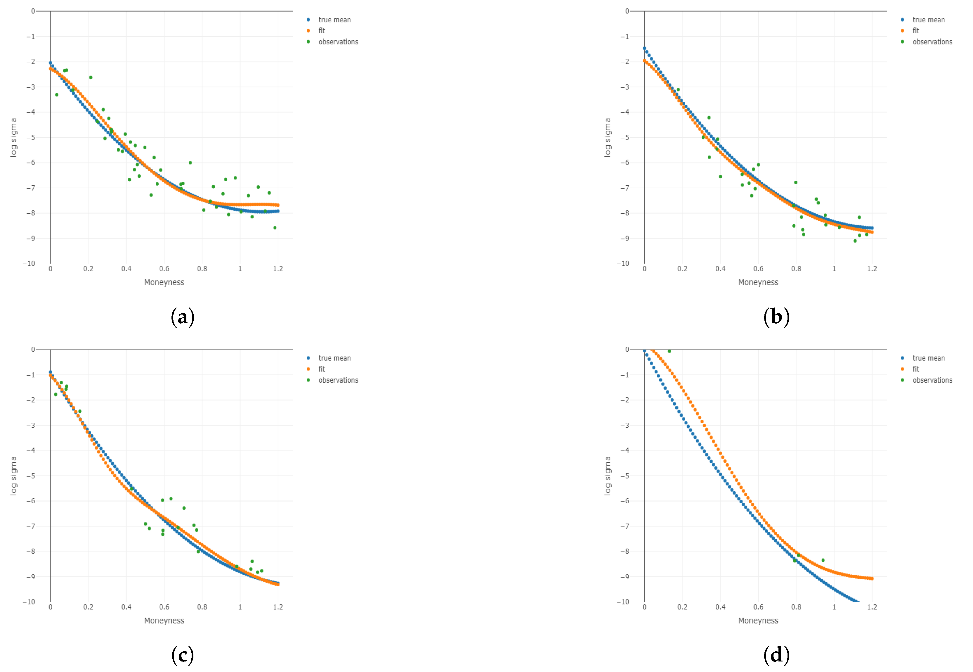
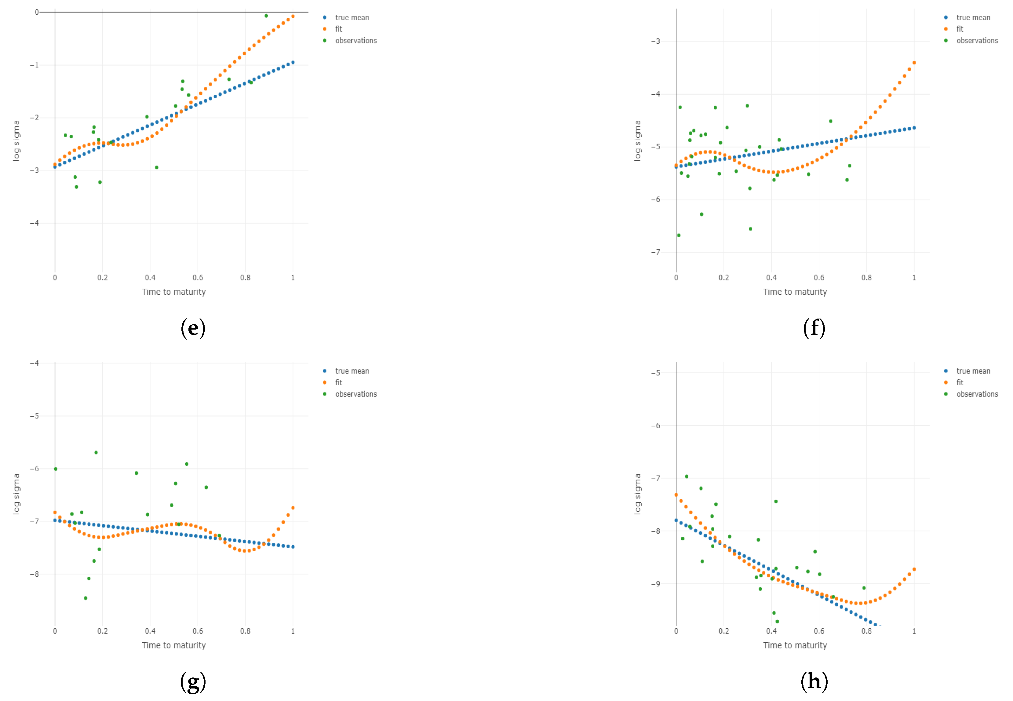
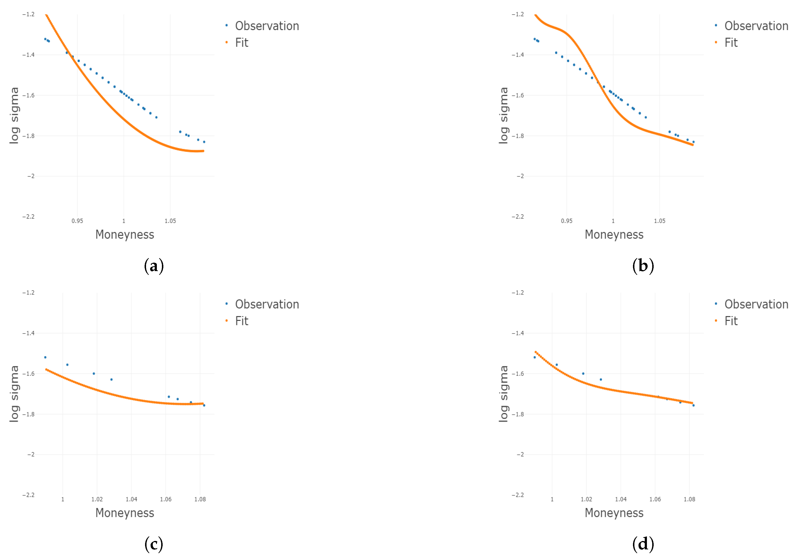
Figure 4.
Two-dimensional plots for different conditional on different and m under . Plots for the 1st, 3rd, 5th, and 8th group are shown conditional on and m, respectively. (a) Two-dimensional plots conditional on the center of the 1st group of ; (b) 2D plots conditional on the center of the 3rd group of ; (c) 2D plots conditional on the center of the 5th group of ; (d) 2D plots conditional on the center of the 8th group of ; (e) 2D plots conditional on the center of the 1st group of m; (f) 2D plots conditional on the center of the 3rd group of m; (g) 2D plots conditional on the center of the 5th group of m; (h) 2D plots conditional on the center of the 8th group of m.
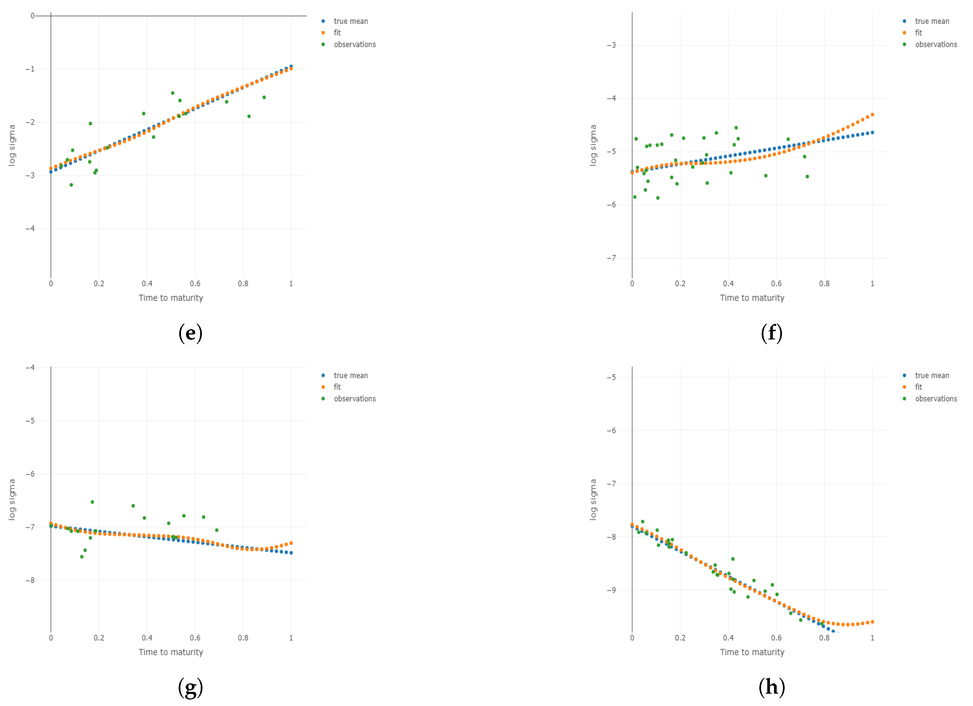
Figure 5.
Two-dimensional plots for different conditional on different and m under . Plots for the 1st, 3rd, 5th, and 8th group are shown conditional on and m, respectively. (a) Two-dimensional plots conditional on the center of the 1st group of ; (b) 2D plots conditional on the center of the 3rd group of ; (c) 2D plots conditional on the center of the 5th group of ; (d) 2D plots conditional on the center of the 8th group of ; (e) 2D plots conditional on the center of the 1st group of m; (f) 2D plots conditional on the center of the 3rd group of m; (g) 2D plots conditional on the center of the 5th group of m; (h) 2D plots conditional on the center of the 8th group of m.
Figure 6.
Two-dimensional plots for different conditional on different and m under . Plots for the 1st, 3rd, 5th, and 8th group are shown conditional on and m, respectively. (a) Two-dimensional plots conditional on the center of the 1st group of ; (b) 2D plots conditional on the center of the 3rd group of ; (c) 2D plots conditional on the center of the 5th group of ; (d) 2D plots conditional on the center of the 8th group of ; (e) 2D plots conditional on the center of the 1st group of m; (f) 2D plots conditional on the center of the 3rd group of m; (g) 2D plots conditional on the center of the 5th group of m; (h) 2D plots conditional on the center of the 8th group of m.
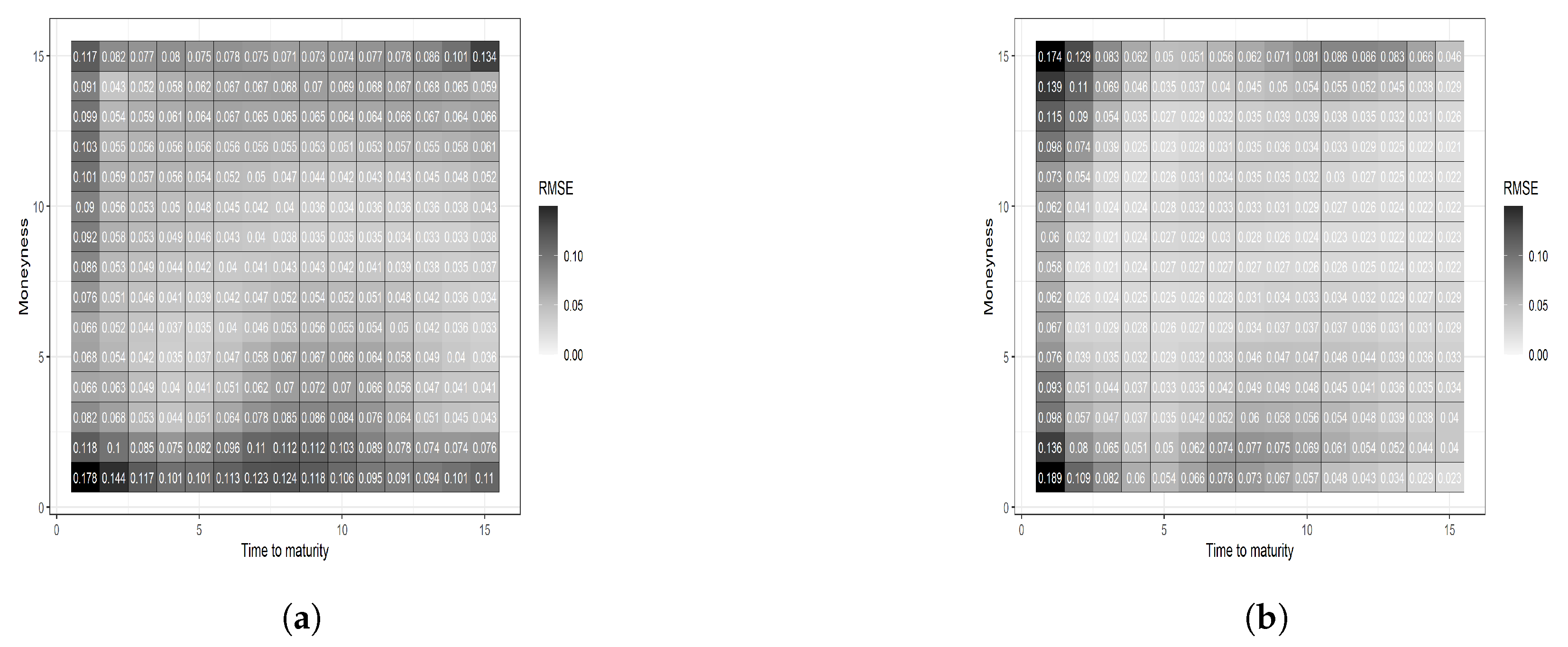
Figure 7.
Two heatmaps are based on a 15 by 15 grid determined by equal-spaced percentiles in moneyness and time to maturity. The parametric benchmark model has a darker area than the additive B-splines model in the bottom, indicating a poorer fit when the moneyness is close its lower boundary. (a) Parametric benchmark; (b) additive B-spline.
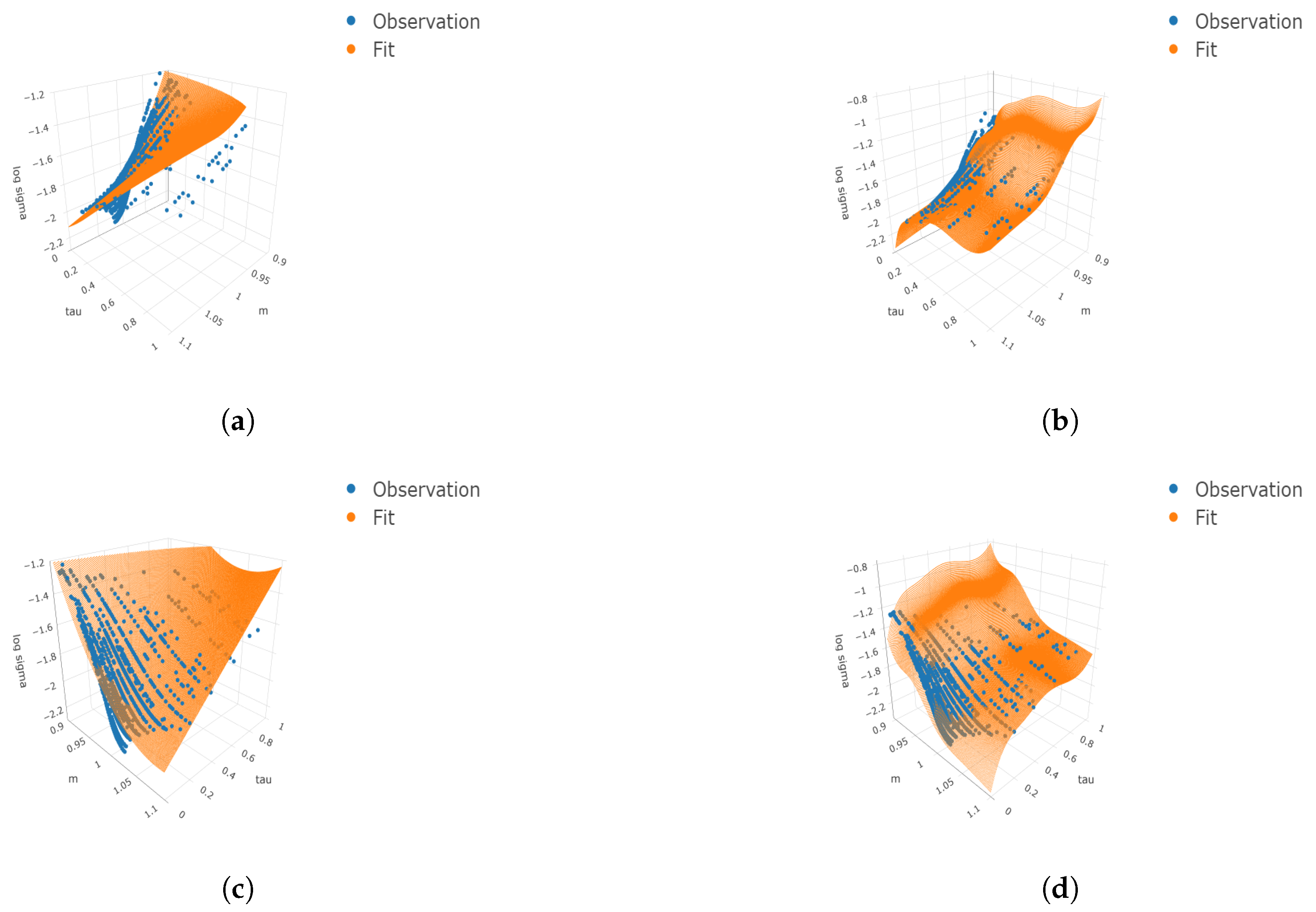
Figure 8.
Four 3D plots with angle 1 and angle 2 compare the in-sample fit of IVS from the parametric benchmark and additive B-splines model on the date 5 February 2021. The additive B-splines model has a better fit to the data. (a) Angle 1 for parametric benchmark, (b) angle 1 for additive B-splines, (c) angle 2 for parametric benchmark, and (d) Angle 2 for additive B-splines.
Figure 9.
Four 3D plots with angle 3 and angle 4 compare the in-sample fit of IVS from the parametric benchmark and additive B-splines model on the date 5 February 2021. The additive B-splines model has a better fit to the data. (a) Angle 3 for parametric benchmark, (b) angle 3 for additive B-splines, (c) angle 4 for parametric benchmark, and (d) angle 4 for additive B-splines.
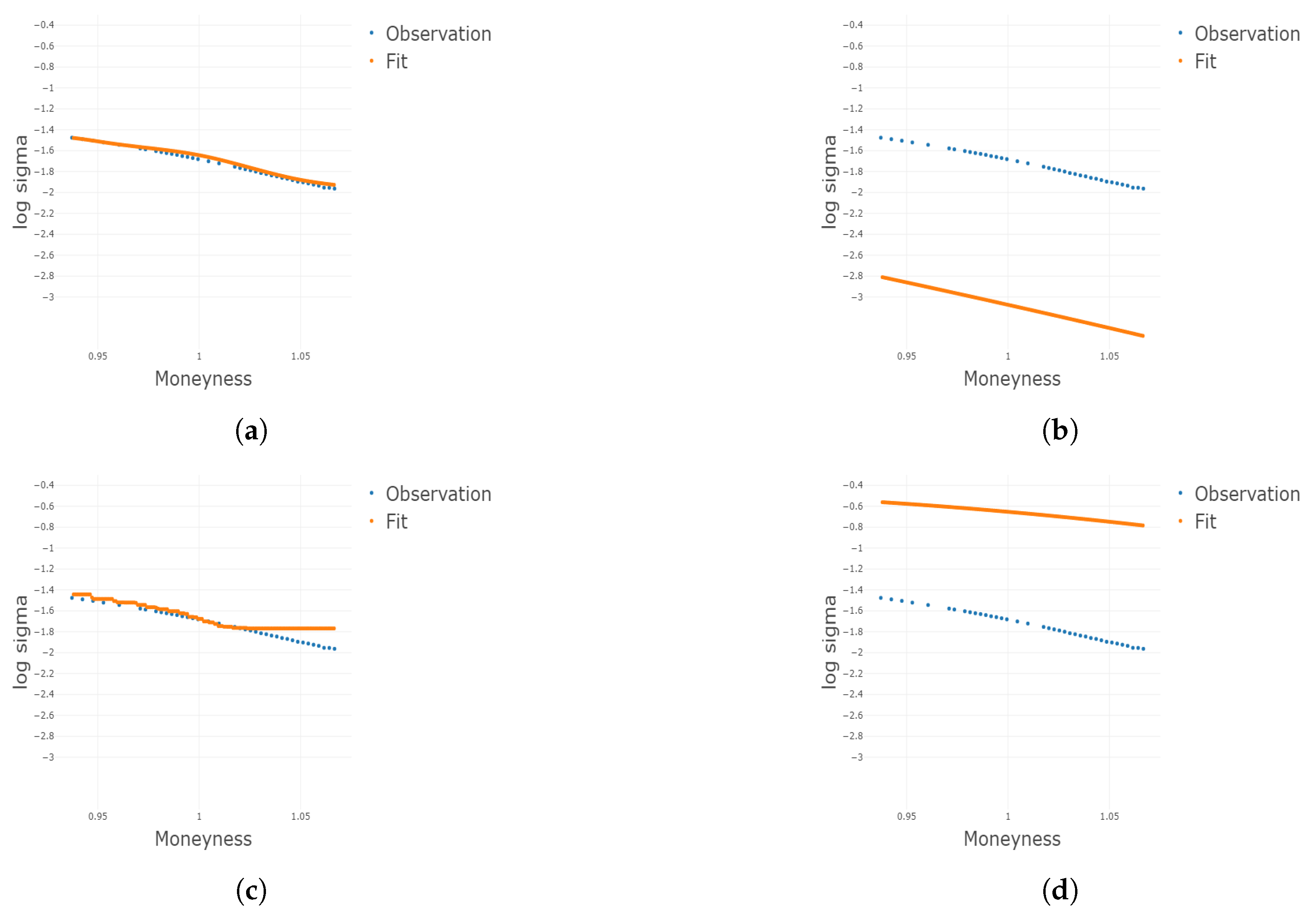
Figure 10.
Four 2D plots conditional on the 20th and 35th percentile of compare the in-sample fit of IVS from the parametric benchmark and additive B-splines model on the date 5 February 2021. The additive B-splines model has a better fit to the data. (a) Parametric benchmark model fit conditional on the 20th percentile, (b) additive B-splines model fit conditional on the 20th percentile, (c) parametric benchmark model fit conditional on the 35th percentile, and (d) additive B-splines model fit conditional on the 35th percentile.
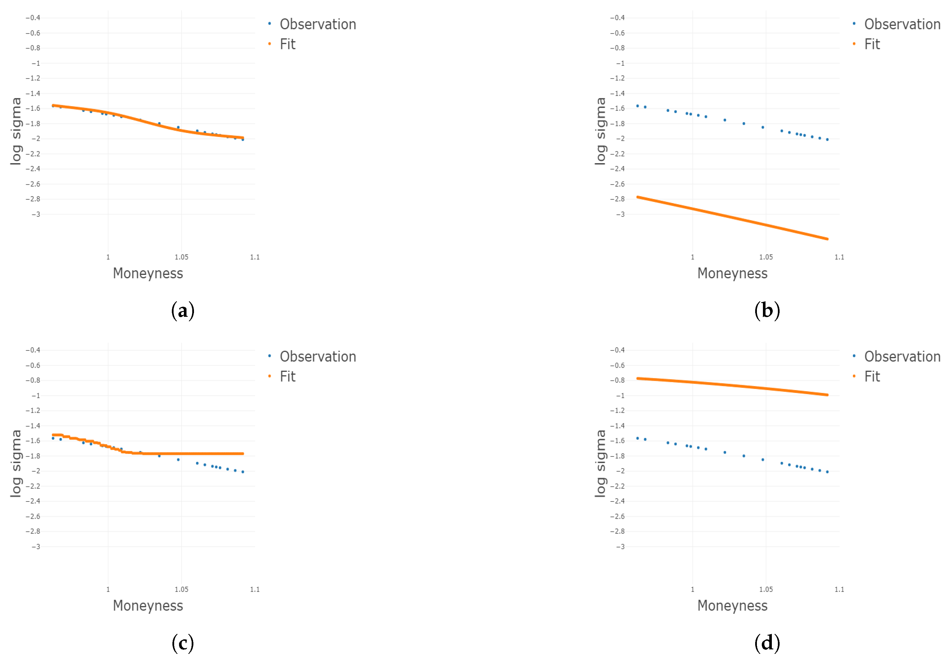
Figure 11.
Four 2D plots conditional on the 65th and 80th percentile of compare the in-sample fit of IVS from the parametric benchmark and additive B-splines model on the date 5 February 2021. The additive B-splines model has a better fit to the data. (a) Parametric benchmark model fit conditional on the 65th percentile, (b) additive B-splines model fit conditional on the 65th percentile, (c) parametric benchmark model fit conditional on the 80th percentile, and (d) additive B-splines model fit conditional on the 80th percentile.
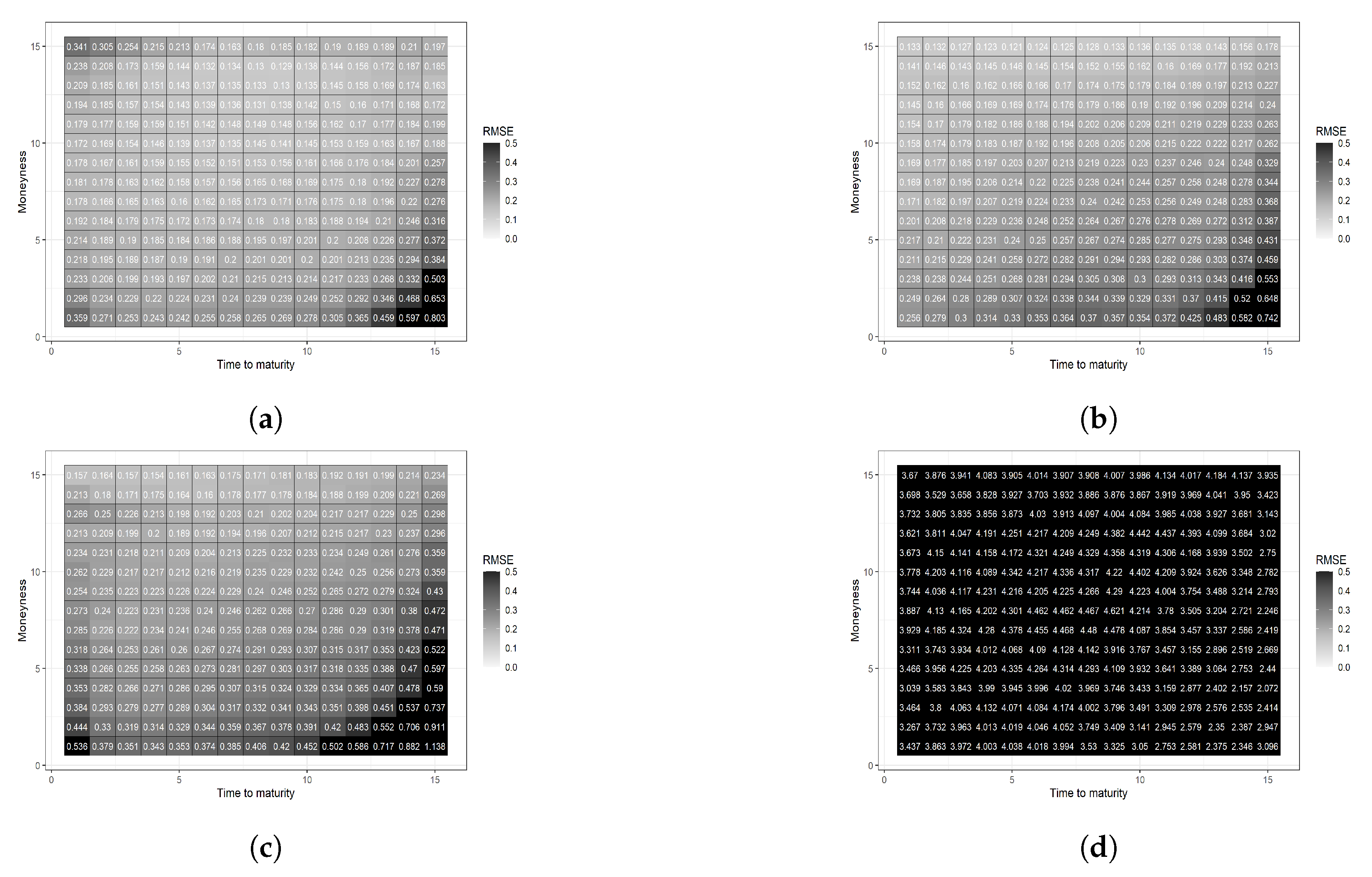
Figure 12.
Four heatmaps are based on a 15 by 15 grid determined by equal-spaced percentiles in moneyness and time to maturity. The dynamic parametric benchmark has the darkest heatmap, while the dynamic additive B-splines model has the brightest, indicating the best fit among the four models. (a) Dynamic additive B-splines model, (b) nonparametric benchmark, (c) parametric benchmark, and (d) dynamic parametric benchmark.
Figure 13.
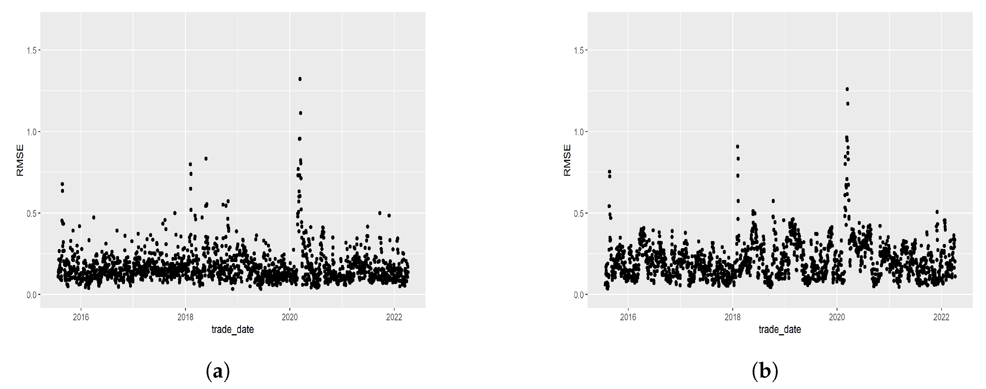
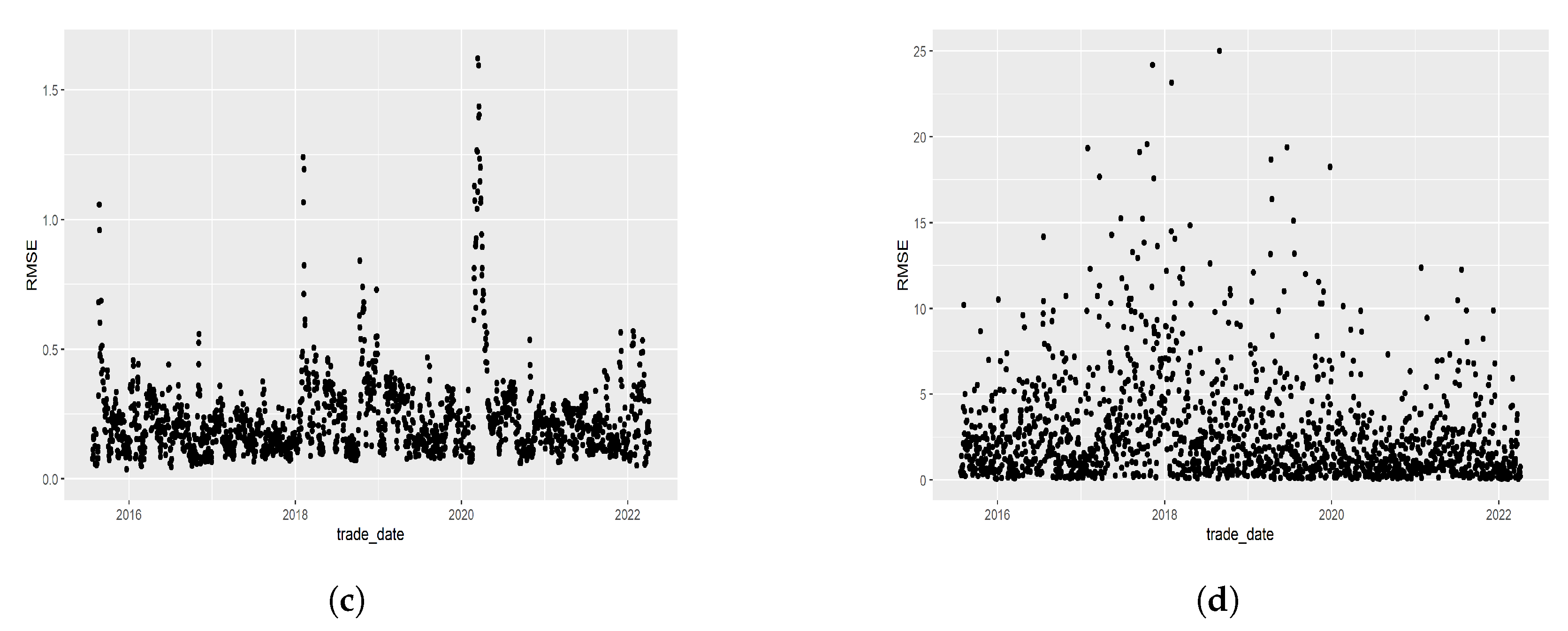
Compare the RMSE time series across the trade date for the four models. The dynamic additive B-splines model has the most stable time series with the narrowest band and fewest extremes, while the dynamic parametric benchmark has the largest spread. (a) RMSE time series for dynamic additive B-splines, (b) RMSE time series for nonparametric benchmark, (c) RMSE time series for parametric benchmark, and (d) RMSE time series for dynamic parametric benchmark.
Figure 13.
Compare the RMSE time series across the trade date for the four models. The dynamic additive B-splines model has the most stable time series with the narrowest band and fewest extremes, while the dynamic parametric benchmark has the largest spread. (a) RMSE time series for dynamic additive B-splines, (b) RMSE time series for nonparametric benchmark, (c) RMSE time series for parametric benchmark, and (d) RMSE time series for dynamic parametric benchmark.
Figure 14.
Four 3D plots with angle 1 compare the in-sample fit of IVS from four models on the date 24 February 2016. The dynamic additive B-splines model has the best fit to the data. (a) Angle 1 for the dynamic additive B-splines model, (b) angle 1 for nonparametric benchmark, (c) angle 1 for parametric benchmark, and (d) angle 1 for dynamic parametric benchmark.
Figure 15.
Four 3D plots with angle 2 compare the in-sample fit of IVS from four models on the date 24 February 2016. The additive B-splines model has the best fit to the data. (a) Angle 2 for the dynamic additive B-splines model, (b) angle 2 for nonparametric benchmark, (c) angle 2 for parametric benchmark, and (d) angle 2 for dynamic parametric benchmark.
Figure 16.
Four 3D plots with angle 3 compare the in-sample fit of IVS from four models on the date 24 February 2016. The dynamic additive B-splines model has the best fit to the data. (a) Angle 3 for the dynamic additive B-splines model, (b) angle 3 for nonparametric benchmark, (c) angle 3 for parametric benchmark, and (d) angle 3 for dynamic parametric benchmark.
Figure 17.
Four 3D plots with angle 4 compare the in-sample fit of IVS from four models on the date 24 February 2016. The dynamic additive B-splines model has the best fit to the data. (a) Angle 4 for the dynamic additive B-splines model, (b) angle 4 for nonparametric benchmark, (c) angle 4 for parametric benchmark, and (d) angle 4 for dynamic parametric benchmark.
Figure 18.
Four 2D plots conditional on the 20th percentile of compare the out-of-sample fit of IVS from four models on the date 24 February 2016. The dynamic additive B-splines model has the best fit to the data. (a) Dynamic additive B-splines model fit conditional on the 20th percentile, (b) parametric benchmark model fit conditional on the 20th percentile, (c) nonparametric benchmark model fit conditional on the 20th percentile, and (d) dynamic parametric benchmark model fit conditional on the 20th percentile.
Figure 19.
Four 2D plots conditional on the 35th percentile of compare the out-of-sample fit of IVS from four models on the date 24 February 2016. The dynamic additive B-splines model has the best fit to the data. (a) Dynamic additive B-splines model fit conditional on the 35th percentile, (b) parametric benchmark model fit conditional on the 35th percentile, (c) nonparametric benchmark model fit conditional on the 35th percentile, and (d) dynamic parametric benchmark model fit conditional on the 35th percentile.
Figure 20.
Four 2D plots conditional on the 45th percentile of τ compare the out-of-sample fit of IVS from four models on the date 24 February 2016. The dynamic additive B-splines model has the best fit to the data. (a) Dynamic additive B-splines model fit conditional on the 45th percentile, (b) parametric benchmark model fit conditional on the 45th percentile, (c) nonparametric benchmark model fit conditional on the 45th percentile, and (d) dynamic parametric benchmark model fit conditional on the 45th percentile.
Figure 21.
Four 2D plots conditional on the 65th percentile of compare the out-of-sample fit of IVS from four models on the date 24 February 2016. The dynamic additive B-splines model has the best fit to the data. (a) Dynamic additive B-splines model fit conditional on the 65th percentile, (b) parametric benchmark model fit conditional on the 65th percentile, (c) nonparametric benchmark model fit conditional on the 65th percentile, and (d) dynamic parametric benchmark model fit conditional on the 65th percentile.
Table 1.
Relative RMSE for four cases of two sample sizes and two levels. There is no significant difference between the different sample sizes under the same level. Therefore, the model performance on the sample is not too sensitive to the sample size.
Table 1.
Relative RMSE for four cases of two sample sizes and two levels. There is no significant difference between the different sample sizes under the same level. Therefore, the model performance on the sample is not too sensitive to the sample size.
| | | |
|---|
| | |
| | |
Table 2.
Relative on grid for four cases of two sample sizes and two levels. Notice that the relative is significantly lower when we have compared with under the same level because the more data, the better fit to the underlying true surface.
Table 2.
Relative on grid for four cases of two sample sizes and two levels. Notice that the relative is significantly lower when we have compared with under the same level because the more data, the better fit to the underlying true surface.
| | | |
|---|
| | |
| | |
Table 3.
This table shows summary statistics for call options in the real data. Note that the time to maturity has the largest skewness and kurtosis, indicating the heavy tail distribution.
Table 3.
This table shows summary statistics for call options in the real data. Note that the time to maturity has the largest skewness and kurtosis, indicating the heavy tail distribution.
| | Mean | Volatility | Skewness | Kurtosis | Min | Max |
|---|
| Implied volatility | −1.9106 | 0.3827 | 0.4528 | 0.5749 | −3.2729 | 0.1913 |
| Moneyness | 1.0086 | 0.0329 | −0.0294 | 0.5207 | 0.8780 | 1.0998 |
| Time to maturity | 0.1439 | 0.1620 | 2.7109 | 8.4048 | 0.0164 | 1.0000 |
Table 4.
The RMSE and relative RMSE are provided for the additive B-splines model and the parametric benchmark model. The additive B-splines model has significantly lower (relative) RMSE and hence provides a better fit of the IVS than the parametric benchmark model.
Table 4.
The RMSE and relative RMSE are provided for the additive B-splines model and the parametric benchmark model. The additive B-splines model has significantly lower (relative) RMSE and hence provides a better fit of the IVS than the parametric benchmark model.
| | Additive B-Splines | Parametric Benchmark |
|---|
| RMSE | 0.0532 | 0.0702 |
| Relative RMSE | 0.0279 | 0.0368 |
Table 5.
Calculate the RMSE for the in-the-money (ITM) options and out-of-money options (OTM) under two models. The additive B-splines model has consistently smaller RMSE.
Table 5.
Calculate the RMSE for the in-the-money (ITM) options and out-of-money options (OTM) under two models. The additive B-splines model has consistently smaller RMSE.
| | Additive B-Splines | Parametric Benchmark |
|---|
| ITM (m < 1) | 0.0424 | 0.0665 |
| OTM (m > 1) | 0.0665 | 0.0756 |
Table 6.
Calculate the RMSE for the overvalued options and undervalued options under two models. The additive B-splines model has consistently smaller RMSE.
Table 6.
Calculate the RMSE for the overvalued options and undervalued options under two models. The additive B-splines model has consistently smaller RMSE.
| | Additive B-Splines | Parametric Benchmark |
|---|
| Overvalued | 0.0564 | 0.0742 |
| Undervalued | 0.0502 | 0.0663 |
Table 7.
The RMSE and relative RMSE are provided for the dynamic additive B-splines, nonparametric benchmark, parametric benchmark, and dynamic parametric benchmark model. The dynamic additive B-splines model has lowest (relative) RMSE, followed by the nonparametric benchmark, parametric benchmark, and dynamic parametric benchmark model.
| | Dynamic Additive B-Splines | Nonparametric Benchmark | Parametric Benchmark | Dynamic Parametric Benchmark |
|---|
| RMSE | 0.2016 | 0.2455 | 0.2962 | 3.8606 |
| Relative RMSE | 0.1057 | 0.1287 | 0.1553 | 2.0242 |
Table 8.
Calculate the RMSE for the in-the-money (ITM) options and out-of-money options (OTM) under the four models. The dynamic additive B-splines model consistently has the lowest RMSE.
Table 8.
Calculate the RMSE for the in-the-money (ITM) options and out-of-money options (OTM) under the four models. The dynamic additive B-splines model consistently has the lowest RMSE.
| | Dynamic Additive B-Splines | Nonparametric Benchmark | Parametric Benchmark | Dynamic Parametric Benchmark |
|---|
| ITM () | 0.2011 | 0.2588 | 0.30971 | 3.7824 |
| OTM () | 0.2022 | 0.2234 | 0.2742 | 3.9781 |
Table 9.
Calculate the RMSE for the overvalued options and undervalued options under two models. The dynamic additive B-splines model has a consistently smaller RMSE. The option is overvalued when the predicted implied volatility is greater than the observed implied volatility.
Table 9.
Calculate the RMSE for the overvalued options and undervalued options under two models. The dynamic additive B-splines model has a consistently smaller RMSE. The option is overvalued when the predicted implied volatility is greater than the observed implied volatility.
| | Dynamic Additive B-Splines | Nonparametric Benchmark | Parametric Benchmark | Dynamic Parametric Benchmark |
|---|
| Overvalued | 0.1813 | 0.2319 | 0.2193 | 3.8242 |
| Undervalued | 0.2303 | 0.2733 | 0.3669 | 3.9086 |


