Analysis of Queueing System with Dynamic Rating-Dependent Arrival Process and Price of Service

Abstract

We consider a multi-server queueing system with a visible queue and an arrival flow that is dynamically dependent on the system’s rating. This rating reflects the level of customer satisfaction with the quality and price of the provided service. A higher rating implies a higher arrival rate, which motivates the service provider to increase the price of the service. A steady-state analysis of this system using the proposed mechanism for changing the rating and a threshold strategy for changing the price is performed. This is carried out via the consideration of a suitably constructed multidimensional Markov chain. The impact of the variation in the threshold defining the strategy for changing the price on the key performance indicators is numerically illustrated. The results can be used to make managerial decisions, leading to an increase in the effectiveness of system operations.

1. Introduction

Currently, there is a high level of competition between service providers in various fields: mobile communications, restaurants, hotels, entertainment, insurance, retail businesses, air transportation, etc. Customers have a wide range of instruments to help them in choosing between providers of similar kinds of services. Among them, the Internet plays an essential role, where a lot of versatile information about the ratings of different providers is available. Platforms such as Google Reviews, Amazon Customer Reviews, TripAdvisor, Skytrax, Traveler, Trustpilot, Zomato, Yelp, Booking, etc., should be mentioned. Ratings are also formed through Web-based consumer opinion platforms (e.g., epinions.com (accessed on 1 April 2024)). The Internet enables customers to share their opinions on, and experiences with, goods and services with a multitude of other consumers, that is, to engage in electronic word-of-mouth (eWOM) communication; see [1]. The concept of eWOM was introduced in the mid-1990s, when the Internet was beginning to change how consumers interacted with each other. eWOM can generally be defined as the sharing and exchange of information among consumers about a product or company via the Internet, social media, and mobile communication.

The rating of any service system reflects customer satisfaction as a measure of the divergence between what customers anticipate from a service or product before they buy it and how they feel about it after using it. Ratings may shift consumers toward higher-rated sellers while simultaneously causing congestion in their service facilities, in particular, long waiting times, refusals in service provisioning, etc. The tasks relating to the account of these phenomena can be solved with the help of queueing theory.

The influence of ratings on the performance of different service providers accounting for possible congestion is widely analyzed in the vast existing literature; see, e.g., [2,3,4,5,6,7,8,9,10,11,12,13]. In [2], the influence of daily deal promotions on online ratings was investigated. In [3], it is noted that customers have to wait for service in many service industries. When customers have a choice, this waiting may influence their service experience, sojourn time, and, ultimately, spending, reneging, and return behavior. The results of [3], based on real statistics, show that a longer waiting time relates to reneging behavior, with a longer time until a customer returns to the system again. The authors of [4] studied the demand and capacity management problem in a restaurant system. A queueing-based optimization model with an underlying state-dependent quasi-birth-and-death process was developed to address the dynamic and nonlinearity difficulties. In particular, the model considered in [4] explicitly captures the demand changes with respect to the system’s congestion state on a near-real-time dynamic basis. In [5], a situation is considered wherein a service provider serves two types of customers: sophisticated and naive. Sophisticated customers are well informed of service-related information and make their joining-or-balking decisions strategically, whereas naive customers do not have such information and rely on online rating information to make such decisions. It is demonstrated that, under certain conditions, a service provider can increase its profitability by simply ‘dancing’ its price, that is, replacing the static pricing strategy with a high–low cyclic pricing strategy. In [6], the relationship between reviews and sales is examined, and the role of reviewer identity disclosure in electronic markets is clarified. The authors of [7] proposed a model to assess service availability based on user tolerance. The availability of a given service is calculated by using the waiting time for it, as well as the varying tolerances that different people have for the waiting time. The findings of [8] reveal that queueing time and staff courtesy are the most important factors (besides cleanliness, seating areas, signage, food services, retail options, and Wi-Fi availability) influencing the overall airport service rating. The research implemented in [8] offers a resource for improving service quality and operational efficiency in the airport industry. In [9], specific guidelines are provided for managerial interventions to improve service quality and guests’ satisfaction for each grading category in hotels in South Africa whose star grading differs. In [10], the multi-server queueing model with additional servers (assistants) providing help to the main servers when they encounter problems is considered a model of real-world systems with customers’ self-service. An arrival flow is assumed to be the essential generalization of the known Markov arrival process in the case of the dynamic dependence of the parameters on the rating of the system. The rating is the process defined at any moment by the quality of service of previously arrived customers. The possibilities of customers’ balking and impatience are taken into account. In [11], a queueing model wherein two service provider systems compete for customers is considered. The comparative rating of two providers is introduced, and customers make a choice between two providers based on this rating. The possibility of increasing the revenue of the service provider via a suitable price alteration corresponding to the change in the rating, which is the focus of the current paper, was not explored in [10,11]. A few summaries of the pertinent literature are available in all the mentioned papers, as well as in [12]. In [12], along with an extensive literature review, a situation is analyzed wherein companies compete with each other on the basis of the waiting time that their customers experience, along with the price they charge for their service.

Besides global ratings, each service provider can create an internal rating. This rating can combine the global rating of the provider available on the Internet with its evaluation of customer satisfaction. Internal ratings can be created in the form of online digital questionnaires, allowing the collection of feedback directly from customers to compile detailed information about several facets of the customer experience. Data from user-generated online material, such as social networking platforms and review websites, can be scraped by the provider. Also, the provider can make the customer survey in different forms: via selective personal oral or written communication, the completion of a questionnaire selectively distributed by the service provider, a customer’s voluntary visit to the provider’s website, etc.

A high global rating of a provider can help to attract more potential customers. The disadvantage of the global rating is that it is formed outside of the provider, and the exact mechanism of rating formation is hardly known. The local rating supported by the provider can be counted using its algorithm and is easily and permanently available to the provider. The analysis of data obtained from customers allows the system manager to identify problems and customer needs, as well as evaluate the effectiveness of system operation. Depending on the customer’s answers, the rating of the system can either increase or decrease. The rating can be used by the provider for the effective management of customer service in the following way. We suppose that information about customer satisfaction (and the rating) is dynamically updated and used by the service provider’s manager. In general, a high rating of the service system is profitable for the service provider. A higher rating causes a higher customer arrival rate, with the potential to obtain greater revenue from each customer service, given a fixed price in this period. At the same time, a high rating of the system is a good reason for the provider to increase the price of the service to obtain more revenue beyond that attributable to the increased arrival rate. Sooner or later, after the rating increases, it may decrease. The reasons for that are clear. The higher arrival rate caused by the rating increase implies, given a fixed number of service devices and service rates, a worse quality of service and, in particular, a higher probability of customer loss due to a refusal to enter the overcrowded system (balking) and due to impatience (abandonment or reneging during the waiting time). Balking and reneging are inherent features of the majority of real-world systems. Balking and reneging, in combination with a higher service price, may eventually lead to a decrease in the rating. This, in turn, will cause a decrease in the arrival rate and the necessity to reduce the price. The dependence of system revenue on the rating and price is quite complicated, and good decisions can hardly be made just based on the experience and intuition of the system manager. Thus, if the system manager would like to choose the appropriate moments at which the price can be increased or has to be decreased, a thorough mathematical analysis of the variants of rating and price choice is required.

In this paper, we consider a reasonable mechanism for local rating counting and a policy for price-level control depending on the current rating of the service system. The system is analyzed via an investigation of a suitably constructed multidimensional Markov chain. The methodology of the implemented analysis can be adopted for various modifications of the mechanisms for rating determination based on counting the admission or rejection of a customer and his or her opinion about the quality of the received service and its price adequacy.

A brief outline of this article’s presentation is as follows. Rating and price formation mechanisms are described in Section 2. The queueing model with rating-dependent arrivals under study is also formulated in this section. In Section 3, a description of the system’s Markov process is given. The block-structured generator of this process is derived, and the derivation is explained. The calculation of the stationary distribution of the system states is briefly covered in Section 4. Formulas for the calculation of its performance measures are also presented in this section. Section 5 contains a numerical example and an illustration of how the obtained results can be used for the optimization of the system operation via the appropriate choice of the thresholds defining the policy for price adjustment. The conclusion is presented in Section 6.

2. Rating and Price Formation Mechanisms and Queueing Model

We consider a queueing system consisting of an infinite buffer and N independent, identical servers. The structure of the system operation and its main components are shown in Figure 1.

We assume that customers arrive at the system in a flow defined by the rating-dependent Markov arrival process ($RMAP$). The $RMAP$ is a generalization of the standard Markov arrival process ($MAP$) (see, e.g., [14,15,16,17,18,19]), which, in turn, is recognized as an essentially general and better model of flows in many real-world scenarios than the stationary Poisson arrival process, which is widely used in the queueing literature. The $MAP$ model of arrivals makes it possible to account for variations in the instantaneous arrival rate and possible dependence on inter-arrival times.

The customer arrival intensity dynamically depends on the current value of the rating of the system. Such a rating is an integer number, which varies in the range from 1 to $R,$ where R is the maximum rating. The arrivals in the $RMAP$ are governed by the irreducible underlying Markov chain ($MC$) ${\nu }_t,t\ge 0,$ whose transition rates depend on the parameter $r,r=\overline{1,R},$ which defines the current rating of the system. The state space of $MC$${\nu }_t$ is the set $\{1,2,\dots ,W\}.$ If the rating of the system is $r,$ then the transition rates are defined by the matrices $D_0^{\left(r\right)}$ and $D_1^{\left(r\right)}$ of size $W.$ The matrix $D_0^{\left(r\right)}$ defines the transition rates of the process ${\nu }_t$ at which customers do not arrive. The matrix $D_1^{\left(r\right)}$ defines the transition rates of the process ${\nu }_t$ at which customer arrivals occur. The average arrival rate of the $RMAP,$ when the rating of the system is $r,$ is denoted by ${\lambda }_r$, which can be defined by

$${\lambda }_r={\mathit{\theta }}^{\left(r\right)}{D}_1^{\left(r\right)}\mathbf{e},r=\overline{1,R},$$

where ${\mathit{\theta }}^{\left(r\right)}$ is an invariant probability vector of the $MAP$ defined by the matrices $D_0^{\left(r\right)}$ and $D_1^{\left(r\right)}$, and $\mathbf{e}={(1,1,\dots ,1)}^T.$ Here and below, a notation like $r=\overline{1,R}$ means that the variable r takes values from the set $\{1,2,\dots ,R\}$.

We do not specify the concrete form of the matrices $D_0^{\left(r\right)}$ and $D_1^{\left(r\right)}.$ We only assume that an increase in rating cannot imply a decrease in the average arrival rate; i.e., we assume the following inequalities to be satisfied:

$${\lambda }_1\le {\lambda }_2\le \dots \le {\lambda }_R.$$

The rating of the system and the price of the service may dynamically change depending on the results of the customer survey. We assume that an arbitrary arriving customer will give his or her opinion, which will be accounted for in the rating update, with the probability b and that the customer will not participate in the survey with the complementary probability $1-b$.

It is assumed that the customer participating in the survey evaluates two items: the length of the queue and the price of the service. The mechanism for changing the rating of the system is as follows. The queue in the system is visible. An arriving customer observes the current length of the queue. This can occur by visually observing the queue, by receiving information from the provider in verbal form, by comparing the number printed on his or her ticket with the number of customers receiving service displayed on the screen, etc. If there are i customers in the system at the arrival moment, the customer joins the system with the probability $q_i$ or refuses to wait and leaves the system forever (balks) with the complementary probability $1-q_i$.

If an interviewed customer enters the buffer when there are i customers in the system, then the following three scenarios are possible. With the probability $a_i^{\left(1\right)},$ the customer judges the queue length as short and increases the system rating by one. With the probability $a_i^{\left(2\right)},$ he or she judges the queue as too long and decreases the rating by one. With the probability $1-a_i^{\left(1\right)}-a_i^{\left(2\right)},$ the customer judges the queue length as acceptable and does not change the rating. If the surveyed customer leaves the system upon arrival, the customer always decreases the system rating by one.

The price of services in the system is dynamically changed as well. The system’s price level is changed in the range from 1 to P, where P corresponds to the maximum price level. At a fixed price level $p,p=\overline{1,P},$ if an interviewed customer is satisfied with the price level, the rating of the system increases by one with the probability $c_p^{\left(1\right)}$. With the probability $c_p^{\left(2\right)},$ an interviewed customer states that the prices are too high, and the rating of the system decreases by one. With the probability $1-c_p^{\left(1\right)}-c_p^{\left(2\right)},$ the interviewed customers are indifferent to the price level, and the rating is not changed.

The mechanism of the dynamic change in pricing is as follows. The current price remains unaltered for an amount of time that is exponentially distributed with the parameter $\gamma ,\gamma >0.$ After this time, the system revises its prices depending on the current rating. The policy of revision is defined by the two integer thresholds $r_1$ and $r_2,$$1\le r_1<r_2\le R.$ If the current rating belongs to the interval $[1,r_1]$ (the rating is relatively low), then the price level is decreased by one if it is not already the minimum. If the current rating is in the interval $[r_2,R]$ (the rating is relatively high), the price level is increased by one if it is not the maximum. The prices are not changed if the system’s rating is in the interval $(r_1,r_2),$ i.e., if the rating is in the middle of the interval.

The customer service time has an exponential distribution with the parameter $\mu ,\mu >0.$

We assume that customers can be impatient and leave the buffer and depart from the system after an exponentially distributed amount of time with the parameter $\alpha$, $\alpha >0.$ Impatience is an important feature of many real-world systems, and, therefore, its consideration is mandatory for building an adequate model of a real system. The literature related to queueing models with customer impatience is quite extensive; see, e.g., [20,21,22,23,24,25].

The quantitative effect of variations in the thresholds $r_1$ and $r_2$ is difficult to estimate intuitively. Therefore, a mathematical analysis of the system is necessary to evaluate this effect if we would like to optimize the quality of the system operation. We provide such an analysis below.

3. The Markov Process Describing the System and the Derivation of Its Generator

Let

$i_t,$$i_t\ge 0,$ be the number of customers in the system;

$r_t,$$r_t=\overline{1,R},$ be the system’s rating,

$p_t,p_t=\overline{1,P},$ be the price level;

${\nu }_t,{\nu }_t=\overline{1,W},$ be the state of the underlying process of the $RMAP$ at time $t,t\ge 0.$

The behavior of the queueing system under study is described by a regular irreducible $MC$ with continuous time:

$${\xi }_t=\{i_t,r_t,p_t,{\nu }_t\},t\ge 0.$$

The irreducibility of this $MC$ follows from the usually imposed assumption of irreducibility of the underlying process ${\nu }_t$ describing the mechanisms for changing ratings and prices, the component $i_t$ is able to transition from any state i to the neighboring states $i-1$ and $i+1.$

Let us renumber the states of the $MC$${\xi }_t$ in the direct lexicographical order of the components $(i_t,r_t,p_t,{\nu }_t)$ and refer to the set of states of the chain having the value i for the first component of the $MC$ as level $i,i\ge 0.$ The set of states of the chain having the values $(i,r)$ for the first and second components of the $MC$ is called the macrostate $(i,r),i\ge 0,r=\overline{1,R}.$

Let us introduce the following denotations.

⊗ is the symbol of the Kronecker product of matrices; see, for example, [26].

${\delta }_{r,r^{\prime }}$ denotes Kronecker’s delta. It is equal to 1 if $r=r^{\prime }$ and equal to 0 otherwise.

$I_n$ is the identity matrix, and $O_n$ is the zero matrix, the dimension of which is indicated by a subscript n if necessary.

$\mathrm{diag}\{c_1,c_2,\dots ,c_n\}$ is the diagonal matrix with the diagonal elements $c_1,c_2,\dots ,c_n.$

$I_r^{-},$$I_r^{+},$ and $I_r^0,r=\overline{1,R},$ are the square matrices of size P and are defined as follows:

$$I_r^{-}=\left\{\begin{array}{cc}\left(\begin{array}{cccccc}1& 0& 0& \dots & 0& 0\\ 1& 0& 0& \dots & 0& 0\\ 0& 1& 0& \dots & 0& 0\\ ⋮& ⋮& ⋮& \ddots & ⋮& ⋮\\ 0& 0& 0& \dots & 1& 0\end{array}\right),\hfill & r=\overline{1,r_1},\hfill \\ O_P,\hfill & r=\overline{r_1+1,R},\hfill \end{array}\right.$$

$$I_r^{+}=\left\{\begin{array}{cc}{O}_P,\hfill & r=\overline{1,r_2-1},\hfill \\ \left(\begin{array}{cccccc}0& 1& 0& \dots & 0& 0\\ 0& 0& 1& \dots & 0& 0\\ ⋮& ⋮& ⋮& \ddots & ⋮& ⋮\\ 0& 0& 0& \dots & 0& 1\\ 0& 0& 0& \dots & 0& 1\end{array}\right),\hfill & r=\overline{r_2,R},\hfill \end{array}\right.$$

$$I_r^0=\left\{\begin{array}{cc}{I}_P,\hfill & r=\overline{r_1+1,r_2-1},\hfill \\ O_P,\hfill & r=\overline{1,r_1}\bigcup r=\overline{r_2,R}.\hfill \end{array}\right.$$

The following assertion is valid.

Theorem 1.

The generator Q of the $MC$${\xi }_t,t\ge 0,$ has the following block tridiagonal structure:

$$Q=\left(\begin{array}{cccccc}{Q}_{0,0}& Q_{0,1}& O& O& O& \dots \\ Q_{1,0}& Q_{1,1}& Q_{1,2}& O& O& \dots \\ O& Q_{2,1}& Q_{2,2}& Q_{2,3}& O& \dots \\ O& O& Q_{3,2}& Q_{3,3}& Q_{3,4}& \dots \\ ⋮& ⋮& ⋮& ⋮& ⋮& \ddots \end{array}\right)$$

(1)

where the non-zero blocks $Q_{i,j},|i-j|\le 1,$ contain the intensities of transitions from level i to level $j.$ They, in turn, consist of sub-blocks ${\left(Q_{i,j}\right)}_{r,r^{\prime }}$ that determine the transition rates from the macrostate $(i,r)$ to the macrostate $(j,r^{\prime }).$

These blocks and sub-blocks are defined as follows:

The diagonal blocks $Q_{i,i},i\ge 0,$ have the form $Q_{i,i}={\left(Q_{i,i}\right)}_{r,r^{\prime }},r,r^{\prime }=\overline{1,R},$ where the non-zero blocks ${\left(Q_{i,i}\right)}_{r,r^{\prime }}$ are given by

$${\left(Q_{i,i}\right)}_{r,r}=I_P\otimes D_0^{\left(r\right)}+(1-b)(1-q_i)I_P\otimes D_1^{\left(r\right)}-\mu \min \{i,N\}{I}_{PW}-\alpha \max \{0,i-N\}{I}_{PW}-$$

$$-\gamma I_{PW}+\gamma (I_r^{-}+I_r^{+}+I_r^0)\otimes I_W+{\delta }_{r,1}b(1-q_i)I_P\otimes D_1^{\left(1\right)},r=\overline{1,R},$$

$${\left(Q_{i,i}\right)}_{r,r-1}=b(1-q_i)I_P\otimes D_1^{\left(r\right)},r=\overline{2,R},$$

The upper diagonal blocks $Q_{i,i+1},i\ge 0,$ have the form $Q_{i,i+1}={\left(Q_{i,i+1}\right)}_{r,r^{\prime }},|r-r^{\prime }|\le 1,r,r^{\prime }=\overline{1,R},$ where the non-zero blocks are given by

$${\left(Q_{i,i+1}\right)}_{r,r}=(1-b)q_i{I}_P\otimes D_1^{\left(r\right)}+{\delta }_{r,1}b{q}_i{a}_i^{\left(2\right)}{I}_P\otimes D_1^{\left(1\right)}+$$

$$+(1-{\delta }_{r,R})b{q}_i(1-a_i^{\left(1\right)}-a_i^{\left(2\right)})I_P\otimes D_1^{\left(r\right)}+{\delta }_{r,R}b{q}_i(1-a_i^{\left(2\right)})I_P\otimes D_1^{\left(R\right)},r=\overline{1,R},$$

$${\left(Q_{i,i+1}\right)}_{r,r+1}=b{q}_i{a}_i^{\left(1\right)}{I}_P\otimes D_1^{\left(r\right)},r=\overline{1,R-1},$$

$${\left(Q_{i,i+1}\right)}_{r,r-1}=b{q}_i{a}_i^{\left(2\right)}{I}_P\otimes D_1^{\left(r\right)},r=\overline{2,R},$$

The subdiagonal blocks $Q_{i,i-1},i\ge 1,$ have the form $Q_{i,i-1}={\left(Q_{i,i-1}\right)}_{r,r^{\prime }},|r-r^{\prime }|\le 1,r,r^{\prime }=\overline{1,R},$ where the non-zero blocks are defined as

$${\left(Q_{i,i-1}\right)}_{r,r}=\alpha \max \{0,i-N\}{I}_{PW}+(1-b)\mu \min \{i,N\}{I}_{PW}+$$

$$+b\mu \min \{i,N\}\mathrm{diag}\{1-c_p^{\left(1\right)}-c_p^{\left(2\right)},p=\overline{1,P}\}\otimes I_W+$$

$$+{\delta }_{r,1}b\mu \min \{i,N\}\mathrm{diag}\{c_p^{\left(2\right)},p=\overline{1,P}\}\otimes I_W+$$

$$+{\delta }_{r,R}b\mu \min \{i,N\}\mathrm{diag}\{c_p^{\left(1\right)},p=\overline{1,P}\}\otimes I_W,r=\overline{1,R},$$

$${\left(Q_{i,i-1}\right)}_{r,r-1}=b\mu \min \{i,N\}\mathrm{diag}\{c_p^{\left(2\right)},p=\overline{1,P}\}\otimes I_W,r=\overline{2,R},$$

$${\left(Q_{i,i-1}\right)}_{r,r+1}=b\mu \min \{i,N\}\mathrm{diag}\{c_p^{\left(1\right)},p=\overline{1,P}\}\otimes I_W,r=\overline{1,R-1}.$$

Proof. 

The theorem is proved by analyzing the intensities of all possible transitions of the $MC$${\xi }_t$ during an infinitesimal period. Since, during such a period, customers enter and are serviced in the system one at a time, the matrices $Q_{i,j},i,j\ge 0,$ are zero matrices for all $i,j$ such that $|i-j|>1.$ This explains the presence of only three block diagonals in formula (1) of the generator $Q.$

The blocks $Q_{i,j},|i-j|\le 1,$ are built from the matrices ${\left(Q_{i,j}\right)}_{r,r^{\prime }}$ containing the transition rates of the $MC$${\xi }_t$ from the macrostate $(i,r)$ to the macrostate $(j,r^{\prime })$, $r,r^{\prime }=\overline{1,R}$.

Let us explain the forms of all these blocks.

The matrices $Q_{i,i},i\ge 0,$ have the non-zero diagonal blocks ${\left(Q_{i,i}\right)}_{r,r},r=\overline{1,R},$ and subdiagonal blocks ${\left(Q_{i,i}\right)}_{r,r-1},r=\overline{2,R}.$ This is explained by the fact that when the number of customers does not change during an interval of infinitesimal length, the system rating can only decrease or remain the same.

The diagonal elements of the diagonal blocks ${\left(Q_{i,i}\right)}_{r,r},r=\overline{1,R},$ of the $Q_{i,i}$ matrices are negative. Their modules determine the intensity of departure of the $MC$${\xi }_t$ from the respective state. The $MC$${\xi }_t$ can exit from its current state in the following cases:

• The underlying process ${\nu }_t$ of the customer’s arrival leaves the current state. The corresponding transition intensities are determined by the modules of the diagonal entries of the matrices $I_P\otimes D_0^{\left(r\right)},r=\overline{1,R}.$
• A customer is serviced. The corresponding transition rates are given by the matrices $\mu \min \{i,N\}{I}_{PW},$$r=\overline{1,R}.$
• A customer reneges (leaves the buffer) due to impatience. The matrices $\alpha \max \{0,i-N\}{I}_{PW},r=\overline{1,R},$ set the corresponding intensities.
• The price level is changed. The transition rates are determined by the diagonal entries of the matrix $\gamma I_{PW}-\gamma (I_r^{-}+I_r^{+}+I_r^0)\otimes I_W,r=\overline{1,R}.$

Note that if the underlying process ${\nu }_t$ makes a transition from some state $\nu$ to the same state with the generation of a customer and (i) the arriving customer refuses to wait, balks (leaves the system), and does not participate in the survey or (ii) the arriving customer refuses to wait, leaves the system, and participates in the survey when the rating of the system is already the lowest ($r=1$), the state of the $MC$${\xi }_t$ does not change. To this end, to the diagonal entries of the matrices ${\left(Q_{i,i}\right)}_{r,r}$, we have to add the diagonal entries of the matrices $(1-b)(1-q_i)I_P\otimes D_1^{\left(r\right)}$ in case (i) and matrices ${\delta }_{r,1}b(1-q_i)I_P\otimes D_1^{\left(1\right)},r=\overline{1,R},$ in case (ii) that define the corresponding intensities.

The off-diagonal entries of the matrices ${\left(Q_{i,i}\right)}_{r,r},r=\overline{1,R},$ of the matrices $Q_{i,i}$ determine the transition rates of the $MC$${\xi }_t$ without changing the values of the components i and r. These transitions are defined by the following:

• The off-diagonal entries of the matrices $I_P\otimes D_0^{\left(r\right)},r=\overline{1,R},$ when the underlying process ${\nu }_t$ makes a jump without a customer generation;
• The off-diagonal entries of the matrices $(1-b)(1-q_i)I_P\otimes D_1^{\left(r\right)},r=\overline{1,R},$ when an arriving customer abandons the system at the entrance and he or she is not surveyed;
• The off-diagonal entries of the matrices ${\delta }_{r,1}b(1-q_i)I_P\otimes D_1^{\left(1\right)},r=\overline{1,R},$ when an arriving customer abandons the system at the entrance and he or she is surveyed, but the system already has the lowest rating;
• The off-diagonal entries of the matrices $\gamma (I_r^{-}+I_r^{+}+I_r^0)\otimes I_W,r=\overline{1,R},$ when the system changes its price level.

The blocks ${\left(Q_{i,i}\right)}_{r,r-1},r=\overline{2,R},$ given by the matrices $b(1-q_i)I_P\otimes D_1^{\left(r\right)}$ contain the rates of transitions of the $MC$${\xi }_t$ occurring when the system rating decreases by one. This can happen only when an arriving customer leaves the system at the entrance due an unwillingness to wait, participates in the survey, and decreases the system rating.

The matrices $Q_{i,i+1},i\ge 0,$ have the non-zero diagonal blocks ${\left(Q_{i,i+1}\right)}_{r,r},$$r=\overline{1,R},$ subdiagonal blocks ${\left(Q_{i,i+1}\right)}_{r,r-1},$$r=\overline{2,R},$ and upper diagonal blocks ${\left(Q_{i,i+1}\right)}_{r,r+1},$$r=\overline{1,R-1}.$ Let us explain the expressions for these blocks.

First, consider the diagonal blocks ${\left(Q_{i,i+1}\right)}_{r,r},r=\overline{1,R},$ that contain the transition rates of the $MC$${\xi }_t$ when the number of customers increases while the system rating remains the same. This can occur when an arriving customer joins the system and one of the following occurs:

• The customer does not participate in the survey. The corresponding transition rates are given by the entries of the matrices $(1-b)q_i{I}_P\otimes D_1^{\left(r\right)},r=\overline{1,R}.$
• The customer participates in the survey and (i) states that the queue length is acceptable and does not change the rating; (ii) considers the queue length too long and wants to decrease the rating, but the system already has the lowest rating; (iii) considers the queue length short and wants to increase the rating, but the system already has the highest rating. The corresponding rates are given by the matrices $(1-{\delta }_{r,R})b{q}_i(1-a_i^{\left(1\right)}-a_i^{\left(2\right)})I_P\otimes D_1^{\left(r\right)}$ in case (i), matrices ${\delta }_{r,1}b{q}_i{a}_i^{\left(2\right)}{I}_P\otimes D_1^{\left(1\right)}$ in case (ii), and matrices ${\delta }_{r,R}b{q}_i(1-a_i^{\left(2\right)})I_P\otimes D_1^{\left(R\right)}$ in case (iii).

Then, consider the blocks ${\left(Q_{i,i+1}\right)}_{r,r+1},r=\overline{1,R-1},$ and ${\left(Q_{i,i+1}\right)}_{r,r-1},r=\overline{2,R},$ defined by the matrices $b{q}_i{a}_i^{\left(1\right)}{I}_P\otimes D_1^{\left(r\right)}$ and $b{q}_i{a}_i^{\left(2\right)}{I}_P\otimes D_1^{\left(r\right)}$, respectively, which specify the transition intensity of the $MC$${\xi }_t$ in the case where an arriving customer joins the system and considers that the system’s rating should be increased or decreased based on the survey’s results.

The subdiagonal blocks $Q_{i,i-1},i\ge 1,$ contain the rates of the $MC$${\xi }_t$ transitions when the number of customers decreases by one. This can occur when a customer leaves the buffer due to impatience or a customer receives service in the system.

The non-zero diagonal blocks ${\left(Q_{i,i-1}\right)}_{r,r},r=\overline{1,R},$ that suit the occasion when the system’s rating does not change are specified by the following matrices:

(a) $\alpha \max \{0,i-N\}{I}_{PW}$ if a customer reneges (leaves the buffer) due to impatience;

(b) $(1-b)\mu \min \{i,N\}{I}_{PW}$ if a customer who received service is not interviewed;

(c) $b\mu \min \{i,N\}\mathrm{diag}\{1-c_p^{\left(1\right)}-c_p^{\left(2\right)},p=\overline{1,P}\}\otimes I_W$ if a customer interviewed after service is indifferent to the price level;

(d) ${\delta }_{r,1}b\mu \min \{i,N\}\mathrm{diag}\{c_p^{\left(2\right)},p=\overline{1,P}\}\otimes I_W$ if a customer interviewed after service states that the prices are too high and the rating of the system can be decreased by one, but the system already has the lowest rating,

(e) ${\delta }_{r,R}b\mu \min \{i,N\}\mathrm{diag}\{c_p^{\left(1\right)},p=\overline{1,P}\}\otimes I_W$ if a customer interviewed after service is satisfied with the price level and the rating of the system can be increased by one, but the system already has the highest rating.

The blocks ${\left(Q_{i,i-1}\right)}_{r,r+1},r=\overline{1,R-1},$ and ${\left(Q_{i,i-1}\right)}_{r,r-1},r=\overline{2,R},$ defined by the matrices $b\mu \min \{i,N\}\mathrm{diag}\{c_p^{\left(1\right)},p=\overline{1,P}\}\otimes I_W$ and $b\mu \min \{i,N\}\mathrm{diag}\{c_p^{\left(2\right)},p=\overline{1,P}\}\otimes I_W$, respectively, contain the transition intensities of the $MC$${\xi }_t$ in the case where the system rating increases or decreases based on the results of the survey of the serviced customer.

The theorem has been proven. □

4. The Stationary Distribution of the System States and the Calculation of Its Performance Measures

The generator Q of the $MC$${\xi }_t$ defined by Formula (1) is a block tridiagonal matrix of infinite size. Therefore, this $MC$ can be classified as a quasi-birth-and-death ($QBD$) process; for a definition, see, e.g., [17,19,27]. Unfortunately, due to the dependence of some probabilities ($q_i,a_i^{\left(1\right)},$ and $a_i^{\left(2\right)}$) defining the behavior of the system on the number of customers present in the system and due to the impatience of customers, the generator does not possess a quasi-Toeplitz property. This means that the values of the blocks $Q_{i,j}$ depend not only on the difference $j-i$ but also on i and j separately. Thus, the constructed $QBD$ does not fit the class of the level-independent $QBD$, for which a coherent theory was formulated by M. Neuts; see his seminal book [27] and also books [17,19].

Fortunately, it is clear that in real-world applications, the mentioned probabilities $q_i,a_i^{\left(1\right)},$ and $a_i^{\left(2\right)}$ have to possess, when the number i of customers staying in the system tends to infinity, the following asymptotic properties: the probability $q_i$ that the customer chooses to enter the system tends to some value q, the probability $a_i^{\left(1\right)}$ that the customer judges the queue length as short tends to some value $a^{\left(1\right)}$, and the probability $a_i^{\left(2\right)}$ that the customer judges the queue length as too long tends to some value $a^{\left(2\right)}.$ The most realistic values of these limit values are $q=0,a^{\left(1\right)}=0,a^{\left(2\right)}=1.$

After imposing the assumption about these limits’ existence, it is possible to prove the following statement.

Lemma 1.

The $MC$${\xi }_t$ falls to the class of Asymptotically Quasi-Toeplitz Markov Chains ($AQTMCs$) introduced in [28]; see also the book [19].

Proof. 

Essentially, the definition of an $AQTMC$ given in [28] requires the existence of limiting matrices ${\mathcal{Q}}_0,{\mathcal{Q}}_1,$ and ${\mathcal{Q}}_2$, defined by

$${\mathcal{Q}}_k=-\underset{i\to \infty }{lim}{(I\circ Q_{i,i})}^{-1}{Q}_{i,i+k-1}+{\delta }_{k,1}I,k=0,1,2,$$

where ∘ means Hadamard’s product of matrices (see, e.g., [29]). Using the explicit form of the blocks of the generator Q, it is possible to check that these limits exist for the $MC$${\xi }_t$ and are defined by the formula

$${\mathcal{Q}}_0=I,{\mathcal{Q}}_1=O,{\mathcal{Q}}_2=O.$$

Thus, the $MC$${\xi }_t$ satisfies the definition of an $AQTMC$. Lemma 1 isproven. □

Theorem 2.

The $MC$${\xi }_t$ is ergodic for all values of parameters of the queueing system under study.

Proof. 

According to [28], the sufficient condition for the ergodicity of an $AQTMC$ is the fulfillment of the inequality

$$\mathbf{y}{\mathcal{Q}}_0\mathbf{e}>\mathbf{y}{\mathcal{Q}}_2\mathbf{e}$$

where the row vector $\mathbf{y}$ is the unique solution of the system

$$\mathbf{y}=\mathbf{y}({\mathcal{Q}}_0+{\mathcal{Q}}_1+{\mathcal{Q}}_2),\mathbf{y}\mathbf{e}=1.$$

Because ${\mathcal{Q}}_0=I$ and ${\mathcal{Q}}_2=O,$ the required inequality is trivially fulfilled. Theorem 2 is proven. □

This implies that the $MC$${\xi }_t$ has a stationary distribution.

Let ${\mathit{\pi }}_i$ be the row vector of stationary probabilities of the states of the $MC$${\xi }_t,$ which constitute the level $i,i\ge 0,$ and let $\mathit{\pi }(i,r)$ be the row vector of stationary probabilities of the states of the $MC$${\xi }_t,$ which constitute the macrostate $(i,r),i\ge 0,r=\overline{1,R}.$ Let the vector $\mathit{\pi }(i,r)$ be partitioned into sub-vectors: $\mathit{\pi }(i,r)=\left(\mathit{\pi }\right(i,r,1),\mathit{\pi }(i,r,2),\dots ,\mathit{\pi }(i,r,P\left)\right).$

The problem of the computation of the vectors of the stationary probabilities ${\mathit{\pi }}_i,i\ge 0,$ as the solution of the infinite system of Chapman–Kolmogorov equations is pretty difficult. But because the $MC$${\xi }_t$ belongs to the class of $AQMTCs$, the numerically stable algorithm developed in [28] can be adopted for the computation of these vectors. More recent modifications of this effective method can be found, e.g., in [30,31].

After computing the vectors ${\mathit{\pi }}_i,i\ge 0,$ it is feasible to calculate several performance metrics for the considered queueing system.

The mean number of customers in the buffer is calculated using the formula

$$L_{buf}=\sum _{i=N+1}^{\infty }(i-N){\mathit{\pi }}_i\mathbf{e}.$$

It is worth noting that, here, the multiplication of the row vector ${\mathit{\pi }}_i$ by the column vector $\mathbf{e}$ corresponds to the summation of the probabilities of the states of the $MC$${\xi }_t$ that belong to level i, and, correspondingly, ${\mathit{\pi }}_i\mathbf{e}$ is the probability that i customers reside in the system at an arbitrary moment, $i\ge 0.$

The mean number of occupied servers is given by

$$N_{serv}=\sum _{i=0}^{\infty }\min \{i,N\}{\mathit{\pi }}_i\mathbf{e}.$$

The mean number of customers in the system is obtained using the formula

$$L=\sum _{i=1}^{\infty }i{\mathit{\pi }}_i\mathbf{e}=L_{buf}+N_{serv}.$$

The average value of the system’s rating is calculated using the formula

$$\overline{R}=\sum _{i=0}^{\infty }\sum _{r=1}^{R}r\mathit{\pi }(i,r)\mathbf{e}.$$

The average price level is equal to

$$\overline{P}=\sum _{i=0}^{\infty }\sum _{r=1}^R\sum _{p=1}^{P}p\mathit{\pi }(i,r,p)\mathbf{e}.$$

The average intensity $\beta$ of the price level change is given by

$$\beta =\gamma \sum _{i=0}^{\infty }\left(\sum _{r=1}^{r_1}\sum _{p=2}^P\mathit{\pi }(i,r,p)\mathbf{e}+\sum _{r=r_2}^R\sum _{p=1}^{P-1}\mathit{\pi }(i,r,p)\mathbf{e}\right).$$

A short explanation of this formula is as follows. The parameter $\gamma ,\gamma >0,$ is the rate of the occurrence of moments of a possible change in price. The expression in brackets is the probability that the rating has to be changed at such a moment. The first summand is the probability that the rating has to be decreased. The second summand is the probability that the rating has to be increased.

The average intensity of the output flow of satisfactorily serviced customers is calculated by the formula

$${\mu }_{out}=\sum _{i=0}^{\infty }\mu \min \{i,N\}{\mathit{\pi }}_i\mathbf{e}.$$

The average rate of system arrivals is calculated as

$$\lambda =\sum _{i=0}^{\infty }\sum _{r=1}^R\mathit{\pi }(i,r)(I_P\otimes D_1^{\left(r\right)})\mathbf{e}.$$

The probability that an arriving customer will find an idle server andstart service as soon as he/she arrives is found by the formula

$$P_{to-serv}=\frac{1}{\lambda }\sum _{i=0}^{N-1}\sum _{r=1}^R{q}_i\mathit{\pi }(i,r)(I_P\otimes D_1^{\left(r\right)})\mathbf{e}.$$

The probability that an arriving customer will find all servers busy and join the buffer is equal to

$$P_{to-buf}=\frac{1}{\lambda }\sum _{i=N}^{\infty }\sum _{r=1}^R{q}_i\mathit{\pi }(i,r)(I_P\otimes D_1^{\left(r\right)})\mathbf{e}.$$

The probability that an arriving customer will abandon the system due to a disinclination to join the system is found by the formula

$$P_{arr-loss}=\frac{1}{\lambda }\sum _{i=0}^{\infty }\sum _{r=1}^R(1-q_i)\mathit{\pi }(i,r)(I_P\otimes D_1^{\left(r\right)})\mathbf{e}.$$

The loss probability of an arbitrary customer who leaves the buffer due to impatience is obtained using the formula

$$P_{imp-loss}=\frac{\alpha L_{buf}}{\lambda }.$$

The loss probability of an arbitrary customer is given by

$$P_{loss}=P_{arr-loss}+P_{imp-loss}=1-\frac{{\mu }_{out}}{\lambda }.$$

Remark 1.

The last formula presents two different ways to compute the probability $P_{loss}.$ This fact can be used for the control, along with other possible means of testing, of the accuracy of computation of the blocks of the generator (1), the vectors of stationary probabilities, and performance measures of the system.

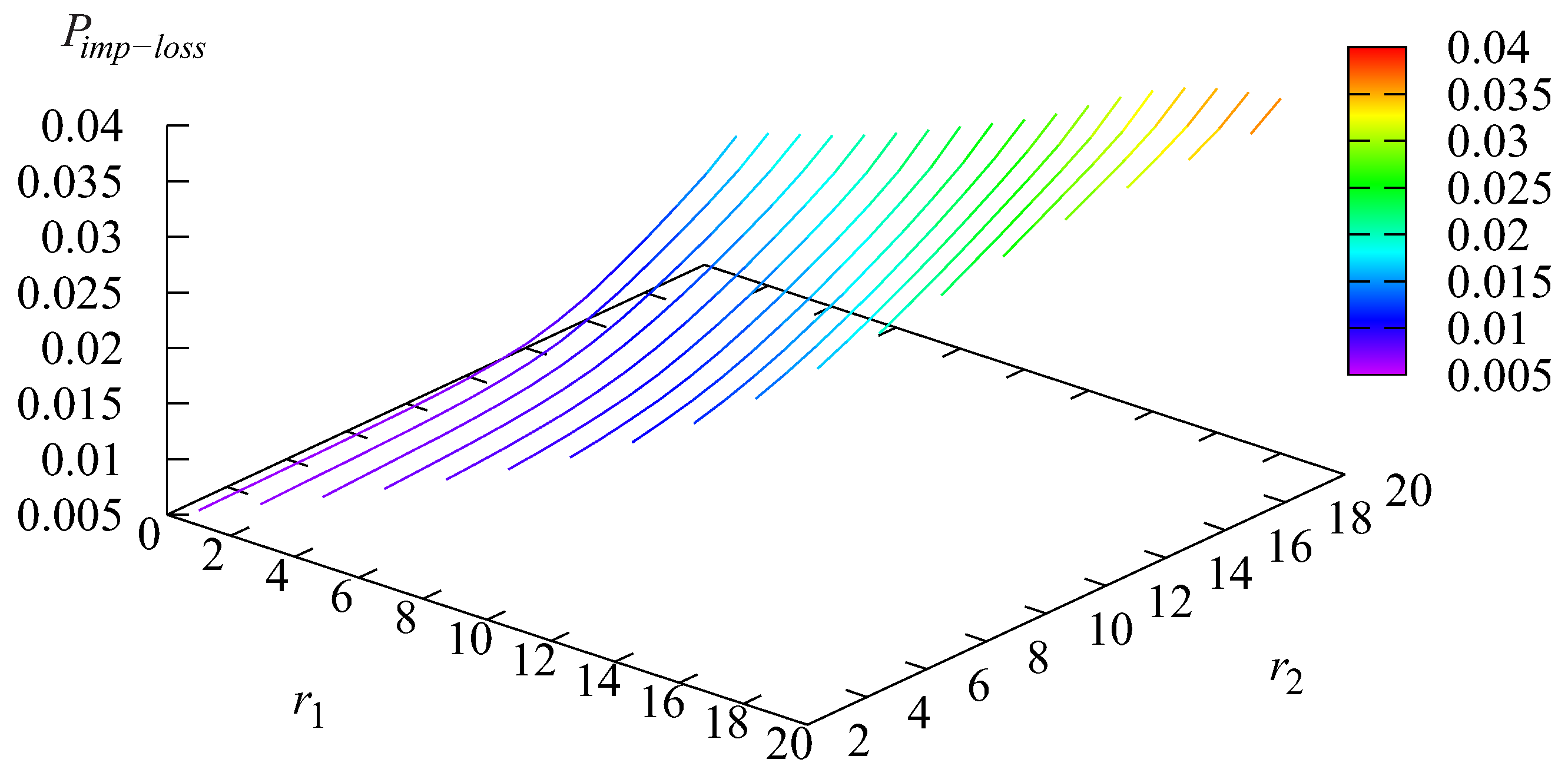
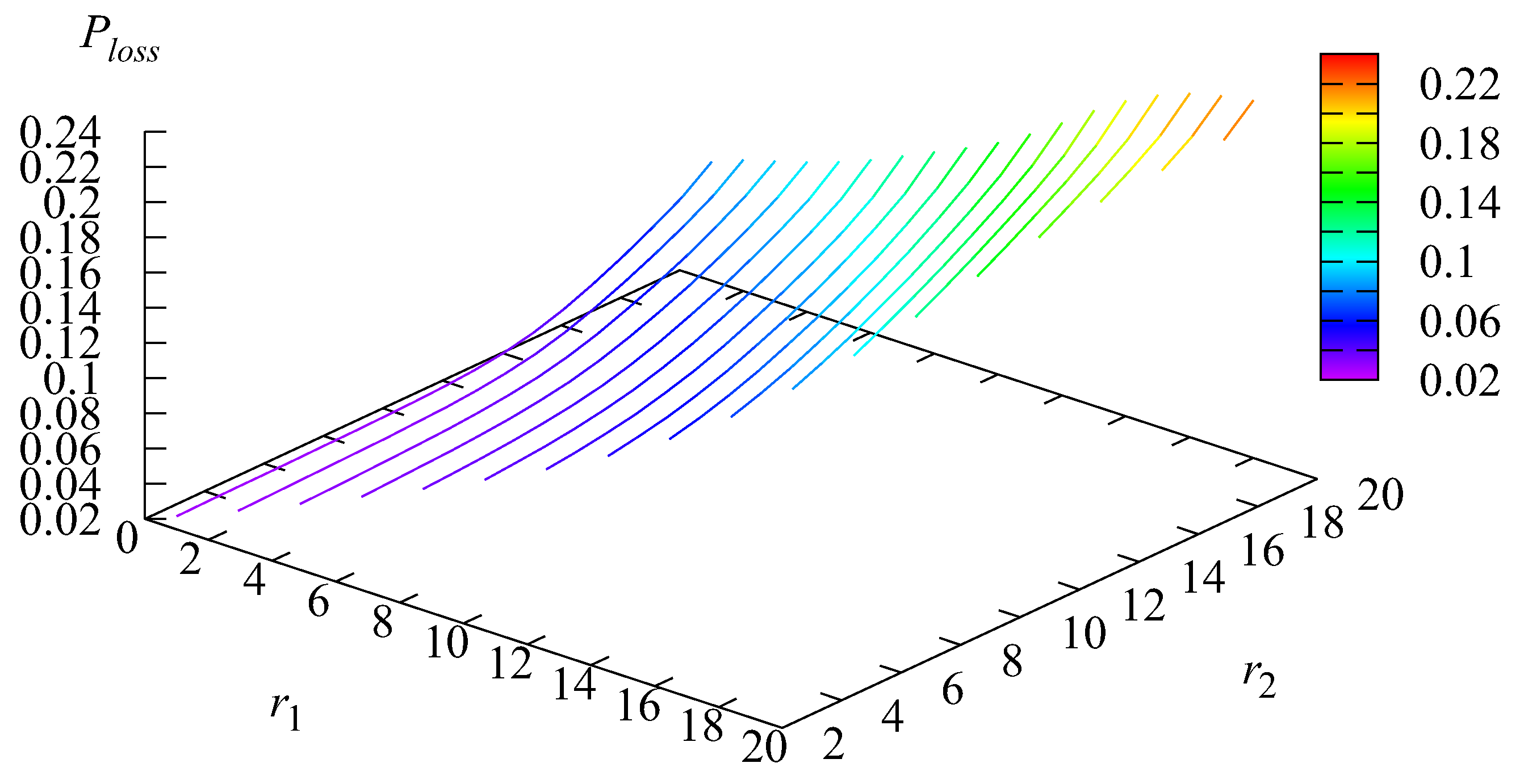
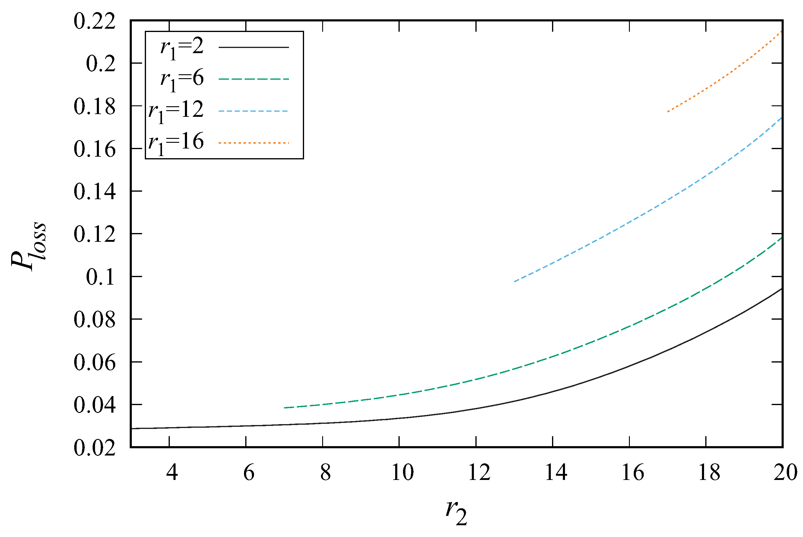
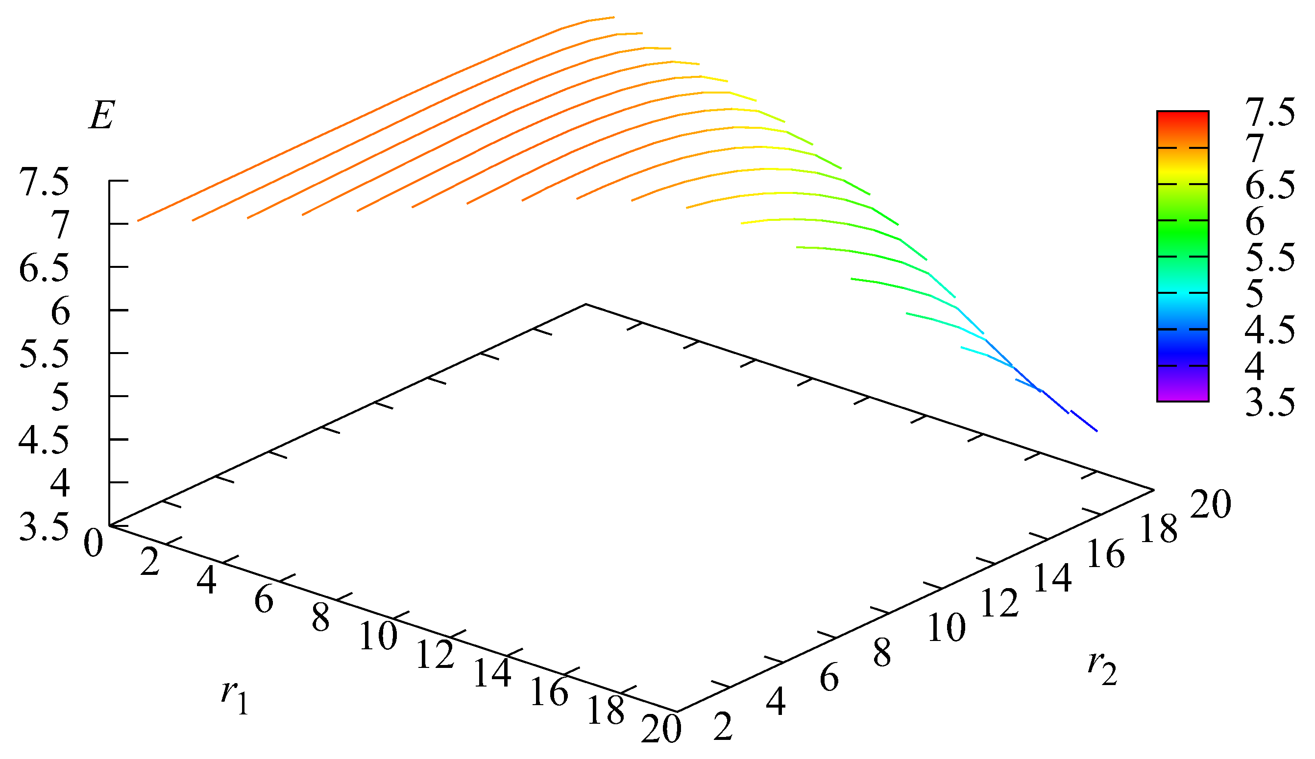
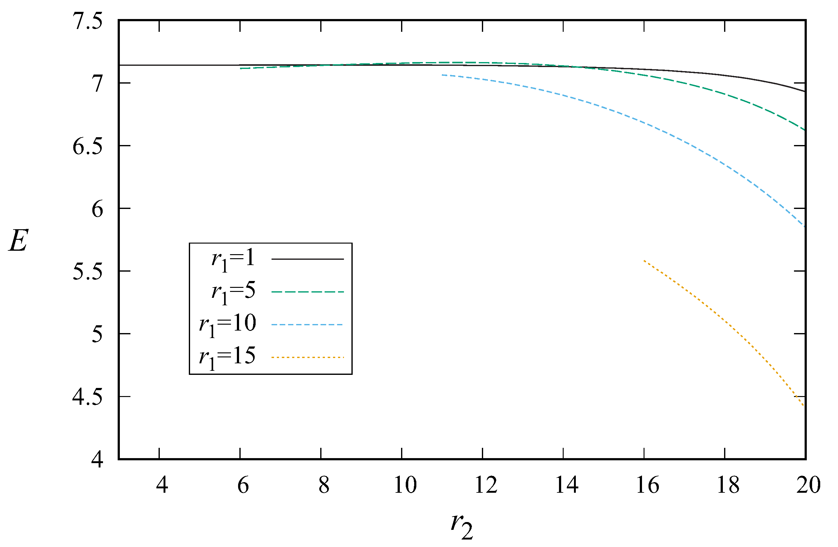
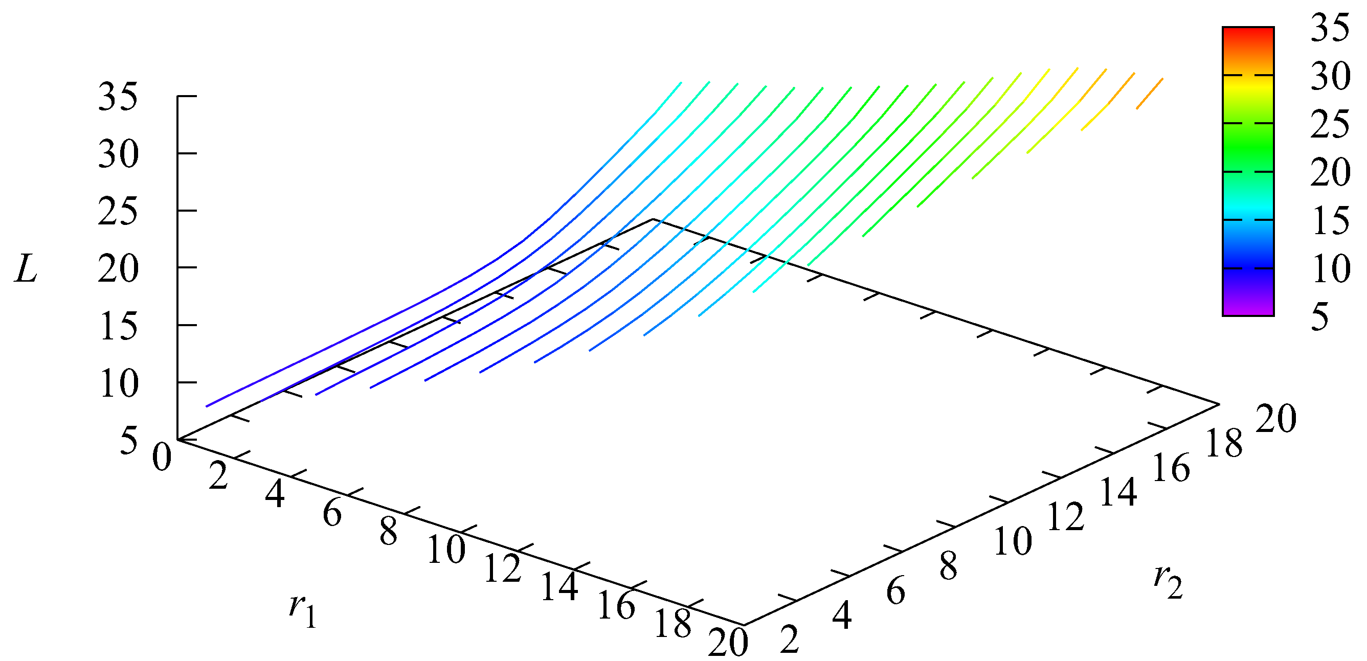
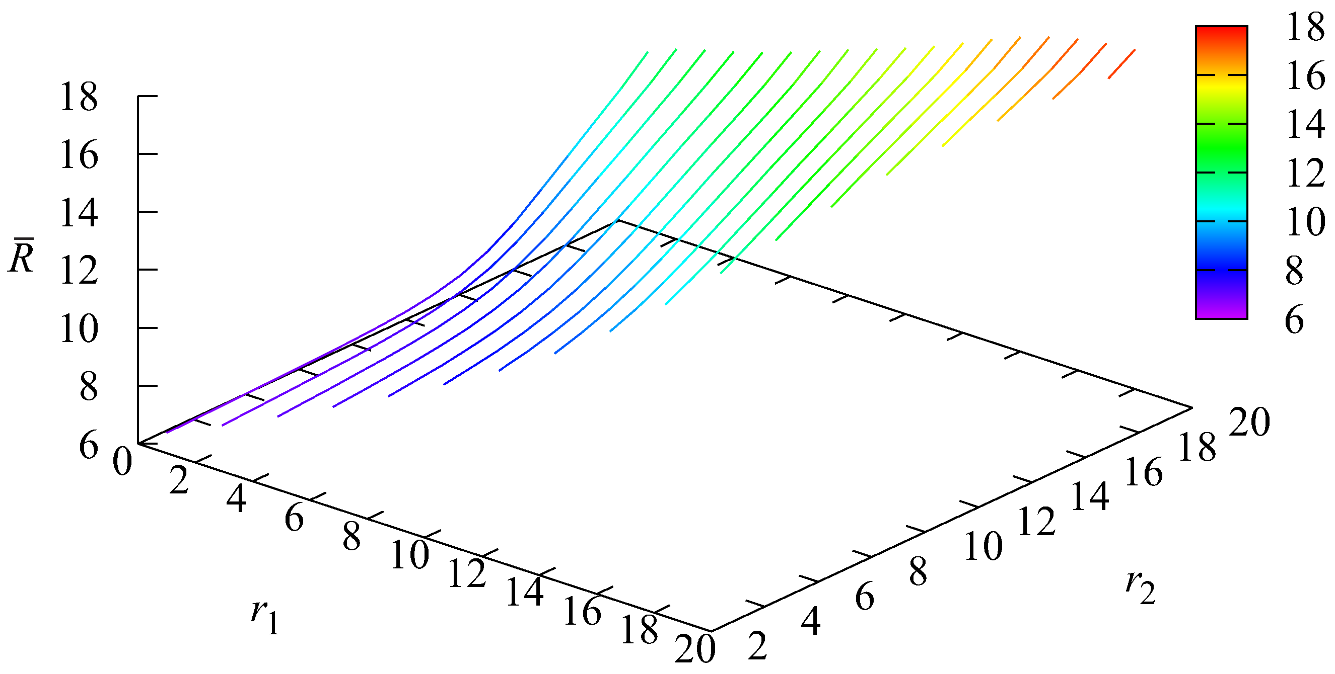
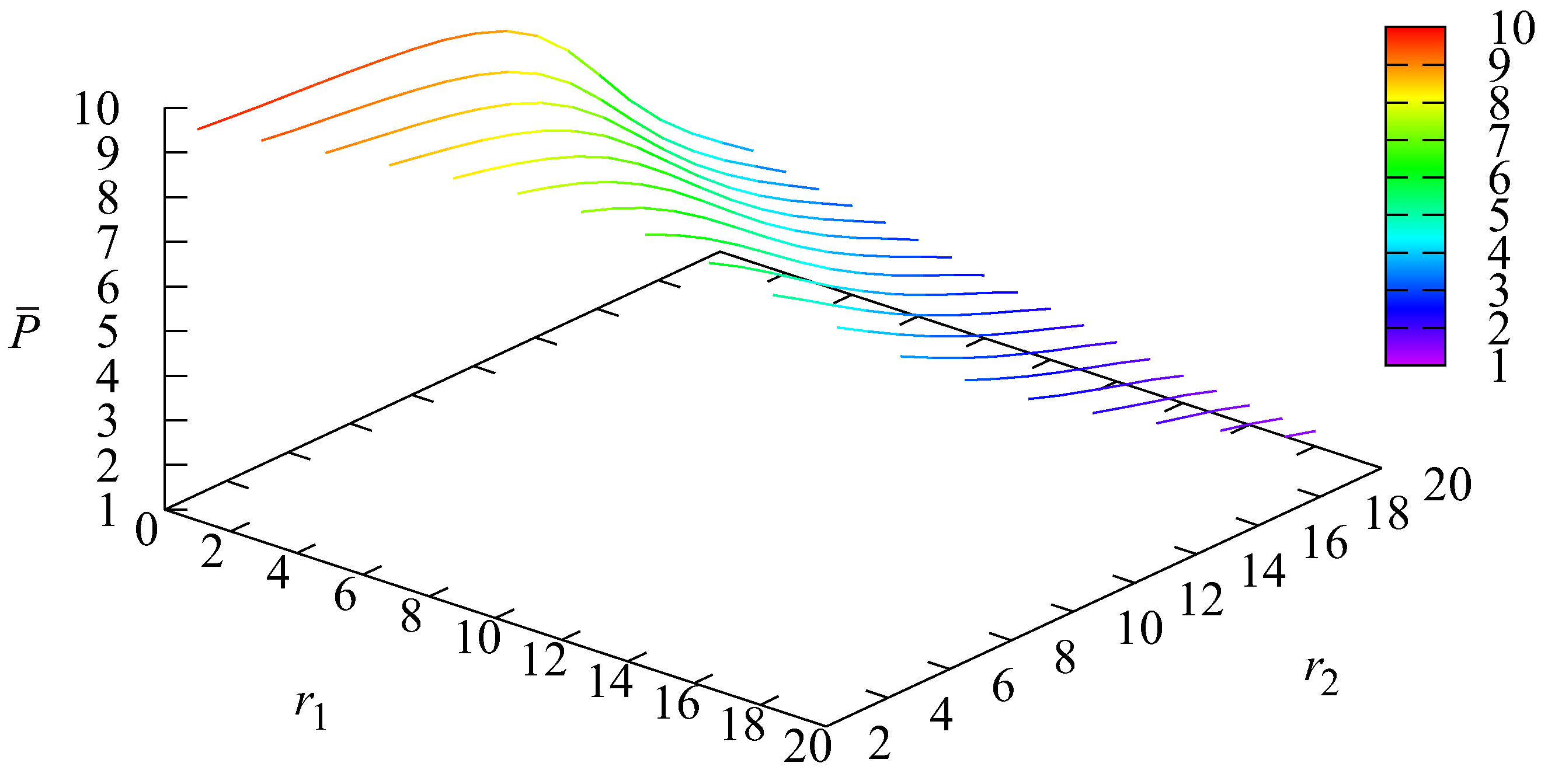
5. Numerical Example

The goals of this numerical example are to highlight the impact of the control parameters $r_1$ and $r_2$ on the key performance measures of the system and to illustrate the possibility of applying the results of the implemented analysis for managerial goals. Unfortunately, we have no access to data from any real system operations. Therefore, in this numerical example, the system’s parameters are selectedbased on common sense.

Consider the base $MAP$, which is defined by the matrices

$$D_0=\left(\begin{array}{cc}-1.77143& 0.0571429\\ 0.0571429& -0.628571\end{array}\right),$$

$$D_1=\left(\begin{array}{cc}1.65714& 0.0571429\\ 0.0114286& 0.56\end{array}\right).$$

This base $MAP$ has the average arrival rate $\tilde{\lambda }=1.$ The coefficient of correlation of the neighboring inter-arrival times is $0.143251,$ and the squared coefficient of variation is $1.52206$.

Let us assume that the rating of the system varies in the range from 1 to R, where $R=20.$ Using the base $MAP,$ we construct the $RMAP$ of customers that arrive at the system. The matrices determined by this $RMAP$ are calculated as follows:

$$D_0^{\left(r\right)}=(1+\frac{r-1}{2})D_0,D_1^{\left(r\right)}=(1+\frac{r-1}{2})D_1,r=\overline{1,20}.$$

When the system rating is r, the average arrival rate of the $RMAP$ is denoted by ${\lambda }_r$ and is calculated by the formula ${\lambda }_r=0.5(r+1),r=\overline{1,20}.$

The number of servers N is considered to be 15, and the service rate $\mu$ is $0.5$. The probability of an arbitrary customer being surveyed b is equal to 0.001.

The probabilities $q_i,a_i^{\left(1\right)}$ and $a_i^{\left(2\right)},i\ge 0,$ are defined as follows:

$$q_i=\left\{\begin{array}{cc}1,\hfill & i<N,\hfill \\ 1-\frac{i-N}{i-N+\frac{3000}{i}},\hfill & i\ge N;\hfill \end{array}\right.$$

$$a_i^{\left(1\right)}=\left\{\begin{array}{cc}1,\hfill & i<N,\hfill \\ 1-\frac{i-N}{i-N+10},\hfill & i\ge N;\hfill \end{array}\right.a_i^{\left(2\right)}=\left\{\begin{array}{cc}0,\hfill & i<N,\hfill \\ \frac{i-N}{i-N+20},\hfill & i\ge N.\hfill \end{array}\right.$$

The system’s price level varies from 1 to P, where $P=10.$ The probabilities $c_p^{\left(1\right)}$ and $c_p^{\left(2\right)},p=\overline{1,10},$ are defined as

$$c_p^{\left(1\right)}=0.9-\frac{p-1}{p},c_p^{\left(2\right)}=0.09+\frac{p-1}{1.2p}.$$

The intensity of the price change $\gamma$ is assumed to be $0.0002$, and the intensity of impatience $\alpha$ is $0.02$.

We vary the rating parameter $r_1$ in the interval $[1,19]$ and the rating parameter $r_2$ in the interval $[r_1+1,20]$ with step 1.

Figure 2, Figure 3 and Figure 4 illustrate the dependence of the average number L of customers in the system, the average number $L_{buf}$ of customers in the buffer, and the average number of busy servers $N_{serv}$ on the parameters $r_1$ and $r_2,$ respectively.

Figure 5, Figure 6, Figure 7 and Figure 8 illustrate the dependence of the average system’s rating $\overline{R}$, the average price level $\overline{P}$, the average arrival intensity $\lambda$, and the average intensity $\beta$ of the price level change on the parameters $r_1$ and $r_2,$ respectively.

As is seen in Figure 2, Figure 3 and Figure 4, the average values L, $L_{buf}$, and $N_{serv}$ decrease with the increase in the parameters $r_1$ and $r_2$. This can be explained as follows. With an increase in the parameter $r_1$, the system rarely decreases the price level, and with an increase in $r_2$, the system rarely increases the price level. As a result, an increase in the parameters $r_1$ and $r_2$ leads to a decrease in the average price level; see Figure 6. From Figure 6, we can conclude that the highest average price level is equal to 9.76246 and is achieved at $r_1=1$ and $r_2=2.$ The minimum average price level is equal to 1.318 and is achieved at $r_1=19$ and $r_2=20.$ As a result, with the increase in the parameters $r_1$ and $r_2$, customers are more often satisfied with the price level, which leads to an increase in the average system rating. Thus, as is seen in Figure 5, the average rating grows with the increase in the parameters $r_1$ and $r_2.$ Note that the minimum rating is achieved at $r_1=1$ and $r_2=2$ and is equal to 6.69775; the maximum value of $\overline{R}$ is 17.79044 for $r_1=19$ and $r_2=20$. Since we assume that the arrival intensity of the $RMAP$ is a nondecreasing function of the rating r, a higher average rating implies a higher average arrival intensity; see Figure 7. The minimum arrival rate is equal to 3.84887 for $r_1=1$ and $r_2=2$ when the average price level is the maximum, and the maximum arrival rate is equal to 9.39522 for $r_1=19$ and $r_2=20$ when the average price level is the minimum. The growth in the average arrival intensity explains the growth in the values L, $L_{buf}$, and $N_{serv}$ with the increase in the parameters $r_1$ and $r_2$.

The dependence of the average intensity $\beta$ of the price level change on the parameters $r_1$ and $r_2$ is quite tricky. We can only conclude that, at a fixed value of $r_1,$ the intensity $\beta$ decreases with the increase in the parameter $r_2,$ and at a fixed value of $r_2,$ the intensity $\beta$ increases with the increase in the parameter $r_2.$ This can be explained as follows. When the rating of the system is in the interval $(r_1,r_2)$, the price level does not change. When the difference between $r_1$ and $r_2$ is bigger, the length of this interval is also bigger, and the system rarely changes the price level, and the intensity $\beta$ decreases. Note that, in the considered example, the maximum value of $\beta$ is 0.00019931 and is achieved when $r_1=12$ and $r_2=13$. The minimum value of $\beta$ is $2.39\times {10}^{-6}$ and is achieved when $r_1=1$ and $r_2=20$.

Figure 9, Figure 10 and Figure 11 illustrate the dependence of the probability $P_{arr-loss}$ that a customer leaves the system upon arrival, the loss probability $P_{imp-loss}$ of an arbitrary customer who leaves the buffer due to impatience, and the total loss probability $P^{loss}$ on the parameters $r_1$ and $r_2,$ respectively.

As one can see from Figure 9, Figure 10, Figure 11 and Figure 12, an increase in the parameters $r_1$ and $r_2$ leads to an increase in all presented loss probabilities. This is a result of raising the average arrival rate $\lambda$ at the system with the increase in the parameters $r_1$ and $r_2.$ The shape of the dependencies looks similar; the difference is only in the values. The minimum values of the loss probabilities are achieved at $r_1=1$ and $r_2=2$ and are equal to $P_{arr-loss}=0.02113$, $P_{imp-loss}=0.00634$, and $P_{loss}=0.02747$. The maximum values of the loss probabilities are achieved at $r_1=19$ and $r_2=20$ and are equal to $P_{arr-loss}=0.18802$, $P_{imp-loss}=0.0372$, and $P_{loss}=0.22522$. Thus, in this numerical example, the total loss probability $P_{loss}$ can vary by about 10 times depending on the values of the parameters $r_1$ and $r_2$. However, the customer loss probability does not always define the quality of the system’s operation since the loss probability does not define the system’s profit.

To be able to estimate the system’s profit and define the optimal values of the control parameters $r_1$ and $r_2$ that maximize the profit, let us assume that the quality of the system’s operation can be described by the cost criterion E, which is defined as follows:

$$E=E(r_1,r_2)=a{\mu }_{out}(1+0.1\overline{P})-c\lambda P_{loss}-d\beta .$$

Here, the parameters a, c, and d are cost coefficients that have the following meaning:

• a is the average profit from servicing one customer.
• c is the charge for the loss of one customer. It may include lost profits and reputational costs.
• d is the charge related to a change in price.

Note that the value $a{\mu }_{out}(1+0.1\overline{P})$ defines the profit obtained by the system per unit of time. The multiplier $(1+0.1\overline{P})$ appears here to account for the fact that if all other parameters’ values are equal, a greater price level implies a greater profit.

Here, we assume that the cost coefficients have the following values:

$$a=1,c=2,d=1000.$$

Figure 13 illustrates the dependence of the cost criterion E on the parameters $r_1$ and $r_2$.

Figure 14 illustrates the corresponding 2D dependence of the cost criterion E on the parameters $r_1$ and $r_2$.

Based on the result of our computations, we can conclude that the optimal value of the cost criterion is $E^{*}=7.17452.$ This value is achieved when $r_1=5$ and $r_2=12.$ In simple words, to obtain the maximum profit, a system manager has to decrease the price level if the rating drops to 5 and increase the price level if the rating is greater than or equal to 12. If the rating of the system is in the interval $[6,11]$ at the moment of a price level reconsideration, the price level has to remain unchanged.

Based on Figure 13 and Figure 14, we can conclude that the cost criterion takes close-to-maximum values when the values of the parameters $r_1$ and $r_2$ are small. When the parameters $r_1$ and $r_2$ are large, the profit significantly decreases. The minimum value of the cost criterion E is 3.89727 for $r_1=19$ and $r_2=20.$ This can be explained by the fact that we chose quite a large value for the coefficient c. Thus, the penalty for a customer loss is severe, and, as was mentioned above, for small values of the parameters $r_1$ and $r_2,$ the loss probability of customers is the minimum. If someone changes the cost coefficients, the shape of the dependence of the cost criterion E on the parameters $r_1$ and $r_2$ may be different. This makes it impossible to predict the optimal values of the parameters $r_1$ and $r_2$ in advance without computations. This explains the necessity of analytical modeling for such systems.

6. Conclusions

In this paper, a rating-counting mechanism for a multi-server queue with an infinite buffer and impatient customers is presented. The rating varies in a fixed, finite range depending on the results of a customer survey. Customers evaluate the degree of their satisfaction by the length of the queue that they encounter upon arrival and by the price of service. A higher rating of the system implies a higher customer arrival rate and the possibility of increasing the price of service. The regulation of the price allows an increase in the revenue of the service provider and implicitly controls the rating and, consequently, the customer’s arrival rate. Customers arrive according to the $RMAP$. The model of the $RMAP$ allows for modeling the arrival process correlated with rating-dependent instantaneous rates.

At fixed thresholds defining the policy for control by price, the behavior of the system is described by a four-dimensional $MC$, with the components including the number of customers in the system, the current rating of the system, the price level, and the underlying process of arrival. An explicit expression for the generator of this $MC$ is obtained. Under realistic assumptions about the form of the dependence of the probabilities of system balking, evaluating the current queue length as too short or too long, the obtained $MC$ belongs to the class of $AQTMCs$ investigated in [19,28,30,31]. This allows us to state that the considered system is always stable and compute its stationary distribution and the key performance indicators of the system. Numerical results confirming the feasibility of the presented formulas and giving insight into the quantitative behavior of the system are presented. The possibility of making the best decision about the thresholds defining the policy for control by price is illustrated.

The obtained results can be expanded to systems with distinct mechanisms for counting ratings and controlling prices. Also, the results can be extended to systems with customer retrials (see, e.g., [32,33,34,35,36]) and, more generally, phase-type distributions (see, e.g., [27,37,38,39]) and the generalized phase-type distribution of service time (see, e.g., [40,41]).

References

1. Hennig-Thurau, T.; Gwinner, K.P.; Walsh, G.; Gremler, D.D. Electronic word-of-mouth via consumer-opinion platforms: What motivates consumers to articulate themselves on the internet? J. Interact. Mark. 2004, 18, 38–52. [Google Scholar] [CrossRef]
2. Bai, X.; Marsden, J.R.; Ross, W.T., Jr.; Wang, G. A note on the impact of daily deals on local retailers’ online reputation: Mediation effects of the consumer experience. Inf. Syst. Res. 2020, 31, 1132–1143. [Google Scholar] [CrossRef]
3. De Vries, J.; Roy, D.; De Koster, R. Worth the wait? How restaurant waiting time influences customer behavior and revenue. J. Oper. Manag. 2018, 63, 59–78. [Google Scholar] [CrossRef]
4. Hwang, J.; Gao, L.; Jang, W. Joint demand and capacity management in a restaurant system. Eur. J. Oper. Res. 2010, 207, 465–472. [Google Scholar] [CrossRef]
5. Huang, F.; Guo, P.; Wang, Y. Cyclic pricing when customers queue with rating information. Prod. Oper. Manag. 2019, 28, 2471–2485. [Google Scholar] [CrossRef]
6. Forman, C.; Ghose, A.; Wiesenfeld, B. Examining the relationship between reviews and sales: The role of reviewer identity disclosure in electronic markets. Inf. Syst. Res. 2008, 19, 291–313. [Google Scholar] [CrossRef]
7. Zhang, K.; Chu, D.; Tu, Z.; Li, C. Service availability assessment model based on user tolerance. Mob. Netw. Appl. 2023, 1–16. [Google Scholar] [CrossRef]
8. Pholsook, T.; Wipulanusat, W.; Ratanavaraha, V. A hybrid MRA-BN-NN approach for analyzing airport service based on user-generated contents. Sustainability 2024, 16, 1164. [Google Scholar] [CrossRef]
9. Nunkoo, R.; Teeroovengadum, V.; Ringle, C.M.; Sunnassee, V. Service quality and customer satisfaction: The moderating effects of hotel star rating. Int. J. Hosp. Manag. 2020, 91, 102414. [Google Scholar] [CrossRef]
10. Dudin, A.; Dudina, O.; Dudin, S.; Gaidamaka, Y. Self-service system with rating dependent arrivals. Mathematics 2022, 10, 297. [Google Scholar] [CrossRef]
11. Dudin, A.N.; Dudin, S.A.; Dudina, O.S.; Samouylov, K.E. Competitive queueing systems with comparative rating dependent arrivals. Oper. Res. Perspect. 2020, 7, 100139. [Google Scholar] [CrossRef]
12. Allon, G.; Federgruen, A. Service competition with general queueing facilities. Oper. Res. 2008, 56, 827–849. [Google Scholar] [CrossRef]
13. Bulatovic, I.; Dempere, J.M.; Papatheodorou, A. The explanatory power of the SKYTRAX’s airport rating system: Implications for airport management. Transp. Econ. Manag. 2023, 1, 104–111. [Google Scholar] [CrossRef]
14. Lucantoni, D. New results on the single server queue with a batch Markovian arrival process. Commun. -Stat. -Stoch. Model. 1991, 7, 1–46. [Google Scholar] [CrossRef]
15. Lucantoni, D.M. The BMAP/G/1 queue: A tutorial. In IFIP International Symposium on Computer Performance Modeling, Measurement and Evaluation; Springer: Berlin/Heidelberg, Germany, 1993; pp. 330–358. [Google Scholar]
16. Chakravarthy, S.R. The batch Markovian arrival process: A review and future work. Adv. Probab. Theory Stoch. Process. 2001, 1, 21–49. [Google Scholar]
17. Chakravarthy, S.R. Introduction to Matrix-Analytic Methods in Queues 1: Analytical and Simulation Approach—Basics; ISTE Ltd.: London, UK; John Wiley and Sons: New York, NY, USA, 2022. [Google Scholar]
18. Chakravarthy, S.R. Introduction to Matrix-Analytic Methods in Queues 2: Analytical and Simulation Approach—Queues and Simulation; ISTE Ltd.: London, UK; John Wiley and Sons: New York, NY, USA, 2022. [Google Scholar]
19. Dudin, A.N.; Klimenok, V.I.; Vishnevsky, V.M. The Theory of Queuing Systems with Correlated Flows; Springer Nature: Cham, Switzerland, 2020. [Google Scholar]
20. Sharma, S.; Kumar, R.; Soodan, B.S.; Singh, P. Queuing models with customers’ impatience: A survey. Int. J. Math. Oper. Res. 2023, 26, 523–547. [Google Scholar] [CrossRef]
21. Bassamboo, A.; Randhawa, R.; Wu, C. Optimally Scheduling Heterogeneous Impatient Customers. Manuf. Serv. Oper. Manag. 2023, 25, 1066–1080. [Google Scholar] [CrossRef]
22. Yin, M.; Yan, M.; Guo, Y.; Liu, M. Analysis of a Pre-Emptive Two-Priority Queuing System with Impatient Customers and Heterogeneous Servers. Mathematics 2023, 11, 3878. [Google Scholar] [CrossRef]
23. Ahmadi, M.; Golkarifard, M.; Movaghar, A.; Yousefi, H. Processor sharing queues with impatient customers and state-dependent rates. IEEE/ACM Trans. Netw. 2021, 29, 2467–2477. [Google Scholar] [CrossRef]
24. Aalto, S. Whittle index approach to multiserver scheduling with impatient customers and DHR service times. Queueing Syst. 2024, 1–30. [Google Scholar] [CrossRef]
25. Liu, H.L.; Li, Q.L. Matched Queues with Flexible and Impatient Customers. Methodol. Comput. Appl. Probab. 2023, 25, 4. [Google Scholar] [CrossRef]
26. Graham, A. Kronecker Products and Matrix Calculus with Applications; Ellis Horwood: Chichester, UK, 1981. [Google Scholar]
27. Neuts, M. Matrix-Geometric Solutions in Stochastic Models; The Johns Hopkins University Press: Baltimore, MD, USA, 1981. [Google Scholar]
28. Klimenok, V.I.; Dudin, A.N. Multi-dimensional asymptotically quasi-Toeplitz Markov chains and their application in queueing theory. Queueing Syst. 2006, 54, 245–259. [Google Scholar] [CrossRef]
29. Horn, R.A.; Johnson, C.R. Topics in Matrix Analysis; Cambridge University Press: Cambridge, UK, 1991. [Google Scholar]
30. Dudin, S.; Dudin, A.; Kostyukova, O.; Dudina, O. Effective algorithm for computation of the stationary distribution of multi-dimensional level-dependent Markov chains with upper block-Hessenberg structure of the generator. J. Comput. Appl. Math. 2020, 366, 112425. [Google Scholar] [CrossRef]
31. Dudin, S.; Dudina, O. Retrial multi-server queuing system with PHF service time distribution as a model of a channel with unreliable transmission of information. Appl. Math. Model. 2019, 65, 676–695. [Google Scholar] [CrossRef]
32. Falin, G.I. A survey of retrial queues. Queueing Syst. 1990, 7, 127–167. [Google Scholar] [CrossRef]
33. Gomez-Corral, A. A bibliographical guide to the analysis of retrial queues through matrix analytic techniques. Ann. Oper. Res. 2006, 141, 163–191. [Google Scholar] [CrossRef]
34. Falin, G.I.; Templeton, J.G.C. Retrial Queues; Chapman & Hall: London, UK, 1997. [Google Scholar]
35. Artalejo, J.R.; Gomez-Corral, A. Retrial Queueing Systems; Springer: Berlin/Heidelberg, Germany, 2008. [Google Scholar]
36. Dudin, A.N.; Manzo, R.; Piscopo, R. Single server retrial queue with group admission of customers. Comput. Oper. Res. 2015, 61, 89–99. [Google Scholar] [CrossRef]
37. Asmussen, S. Applied Probability and Queues; Springer: New York, NY, USA, 2003; Volume 2. [Google Scholar]
38. He, Q.M.; Alfa, A.S. Space reduction for a class of multidimensional Markov chains: A summary and some applications. INFORMS J. Comput. 2018, 30, 1–10. [Google Scholar] [CrossRef]
39. O’Cinneide, C.A. Characterization of phase-type distributions. Stoch. Model. 1990, 6, 1–57. [Google Scholar] [CrossRef]
40. Wu, B.; Cui, L.; Fang, C. Generalized phase-type distributions based on multi-state systems. IISE Trans. 2020, 52, 104–119. [Google Scholar] [CrossRef]
41. Dudin, A.; Kim, C.; Dudina, O.; Dudin, S. Multi-server queueing system with a generalized phase-type service time distribution as a model of a call center with a call-back option. Ann. Oper. Res. 2016, 239, 401–428. [Google Scholar] [CrossRef]
Figure 1. The structure of the system.
Mathematics 12 01101 g001
Figure 2. The dependence of the average number L of customers in the system on the parameters r 1 and r 2 .
Mathematics 12 01101 g002
Figure 3. The dependence of the average number L b u f of customers in the buffer on the parameters r 1 and r 2 .
Mathematics 12 01101 g003
Figure 4. The dependence of the average number N s e r v of busy servers on the parameters r 1 and r 2 .
Mathematics 12 01101 g004
Figure 5. The dependence of the average system’s rating R ¯ on the parameters r 1 and r 2 .
Mathematics 12 01101 g005
Figure 6. The dependence of the average price level P ¯ on the parameters r 1 and r 2 .
Mathematics 12 01101 g006
Figure 7. The dependence of the average arrival rate λ on the parameters r 1 and r 2 .
Mathematics 12 01101 g007
Figure 8. The dependence of the average intensity β of the price level change on the parameters r 1 and r 2 .
Mathematics 12 01101 g008
Figure 9. The dependence of the probability P a r r l o s s that a customer leaves the system upon arrival on the parameters r 1 and r 2 .
Mathematics 12 01101 g009
Figure 10. The dependence of the loss probability P i m p l o s s of an arbitrary customer who leaves the buffer due to impatience on the parameters r 1 and r 2 .
Mathematics 12 01101 g010
Figure 11. The dependence of the loss probability P l o s s on the parameters r 1 and r 2 .
Mathematics 12 01101 g011
Figure 12. The 2D dependence of the loss probability of P l o s s on the parameter r 2 , r 2 > r 1 , for several values of the parameter r 1 .
Mathematics 12 01101 g012
Figure 13. The dependence of the cost criterion E on the parameters r 1 and r 2 .
Mathematics 12 01101 g013
Figure 14. The 2D dependence of the cost criterion E on the parameter r 2 , r 2 > r 1 , for several values of the parameter r 1 .
Mathematics 12 01101 g014
Disclaimer/Publisher’s Note: The statements, opinions and data contained in all publications are solely those of the individual author(s) and contributor(s) and not of MDPI and/or the editor(s). MDPI and/or the editor(s) disclaim responsibility for any injury to people or property resulting from any ideas, methods, instructions or products referred to in the content.