Abstract
Asymptotic synchronization requires continuous external control of the system, which is unrealistic considering the cost of control. Adaptive control methods have strong robustness to uncertainties such as disturbances and unknowns. On the other hand, for finite-time synchronization, if the initial value of the system is unknown, the synchronization time of the finite-time synchronization cannot be estimated. This paper explores the finite-time adaptive synchronization (FTAS) and fixed-time synchronization (FDTS) of fractional-order memristive cellular neural networks (FMCNNs) with time-varying delays (TVD). Utilizing the properties and principles of fractional order, we introduce a novel lemma. Based on this lemma and various analysis techniques, we establish new criteria to guarantee FTAS and FDTS of FMCNNs with TVD through the implementation of a delay-dependent feedback controller and fractional-order adaptive controller. Additionally, we estimate the upper bound of the synchronization setting time. Finally, numerical simulations are conducted to confirm the validity of the finite-time and fixed-time stability theorems.
Keywords:
finite-time adaptive synchronization; fixed-time synchronization; fractional-order memristive cellular neural networks; time-varying delays MSC:
68T07
1. Introduction
Memristive neural networks (MNNs) have garnered significant research interest due to their applications in various fields, including image processing, combinatorial optimization, and artificial intelligence (see [1,2,3]). Differing from traditional neural networks, MNNs are an enhanced version where conventional resistors are substituted with memristors. It is well established that a memristor is a type of resistor possessing memory capabilities, and it can memorize the route through an electric charge [4]. This category of dynamical systems is characterized by state-dependent switched discontinuous systems, which can readily result in complex behaviors and switching uncertainties. Therefore, the dynamical analysis of MNNs is a crucial area of study in both theoretical and applied contexts (see [5,6]). It is widely acknowledged that fractional-order neural networks possess numerous advantages over their integer-order counterparts. Subsequently, fractional-order neural networks have garnered significant interest from researchers, leading to a wealth of insightful findings regarding their dynamical behaviors (see [7,8,9]).
Cellular neural networks (CNNs) are large-scale nonlinear analog circuits that process signals in real time. CNNs are composed of regularly spaced cells. However, as the number of cells in the CNNs increases, the circuit structure of the CNNs becomes complex, which can make it inconvenient to update the weight templates. If memristors are used to implement synaptic connections within the CNNs, it can reduce area consumption and power consumption, and the conditions for updating weights become simpler. Due to the inherent memory characteristics of memristors, the information processing capabilities of the memristor cellular neural networks (MCNNs) are enhanced (see [10,11]).
Fractional calculus is an extension of integer calculus. It is characterized by taking into account the current state and all previous states, exhibiting a memory property. It is widely used as a mathematical tool in fields such as pattern recognition, information processing, robot control, physics, statistics, and more. In practical applications, the fractional order is often used to establish neural network models (see [12,13,14,15,16]).
In the practical application of neural networks, the processing and transmission of signals between neurons are limited by the switching speed of amplifiers. A time delay is inevitable, which affects the stability of the neural network and leads to divergence, instability, and oscillation of the network system. Delays include constant delays and time-varying delays, which are considered more effective than constant delays in establishing neural network systems. Neural networks with TVD are more capable of solving complex practical problems (see [17,18,19,20]).
Synchronization refers to the dynamic behavior wherein a system, through processes of driving and responding, achieves a state of congruence after a specified duration. Synchronous technology, with its potential applications in medicine, information science, optimization computing, and automatic control, has garnered significant attention in recent years. It assumes multiple forms, for instance, asymptotical synchronization [21,22], exponential synchronization [23,24], robust synchronization [25], finite-time synchronization [26,27,28,29,30,31], fixed-time synchronization [32,33,34,35], and so on. In practical applications, due to objective constraints, we usually hope to achieve synchronization of the neural network drive response within a limited time. Furthermore, the finite-time and fixed-time control techniques have also demonstrated superior interference suppression performance and robustness.
In recent years, there have been significant advancements in the study of finite-time synchronization (FTS) for memristive neural network systems. For instance, see [36,37,38,39,40,41,42,43]. Li et al. [36] investigated FTS for a class of drive-response FMNNs with discontinuous activation functions. Li et al. [37] explored the FTS and FDTS of coupled MNNs with discontinuous feedback functions. Li et al. [38] discussed the FTAS and FTS of MNNs with discontinuous activation functions and mixed time-varying delays. Zhang et al. [39] studied the FTS of fractional-order complex-valued MNNs with delay. Guo et al. [40] proposed FTS of drive-response inertial MNNs with time delay. Wei et al. [41], utilizing interval-matrix-based methods, investigated the FTS/FTDS of delayed inertial MNNs. Gong et al. [42] focused on the FTS problem of fuzzy MNNs with time delay. Zhao et al. [43] investigated FTS for a class of FOMFNNs with leakage and transmission delays.
However, independent of initial conditions, finite-time synchronous control methods cannot ensure the system’s convergence within a predetermined time frame. When the initial state information is unknown, the application of these methods becomes restricted by the lack of initial conditions. Researchers have initiated investigations into the issue of the FDTS control problem and have attained preliminary findings. For instance, Arslan et al. [44] investigated the controller design problem for FTDS of fractional-order memristive complex-valued BAM neural networks. Wang et al. [45], utilizing a fractional-order sliding-mode control method, investigated the FDTS control problem of MNNs. Xiao et al. [46] discussed the FDTS control problem of memristive neural networks with delay. Wang et al. [47], utilizing impulsive effects via the novel fixed-time stability theorem, investigated the FDTS control problem of memristive neural networks with delay. Although MNNs have achieved good results in finite-time synchronization and fixed-time synchronization, there is still a lack of research on finite-time and fixed-time synchronization of FMNNs, especially for FMNNs with mixed time-varying delays, which has driven our investigation.
As far as the author knows, the FTAS and FDTS of FMCNNs with TVD have not been fully studied. The main contributions of this article are summarized as follows:
- For the first time, the FTAS and FDTS of FMCNNs with TVD are studied. In practical applications, FTAS and FDTS are more general and practical than finite-time synchronization and asymptotic synchronization;
- By constructing a nonlinear feedback controller and choosing a simple Lyapunov function, some sufficient conditions which are easy to verify are obtained to ensure the finite-time and fixed-time stability of FMCNNs and the FTAS and FDTS of the drive-response FMCNNs systems;
- The theoretical results obtained are more general and can improve or supplement previous results effectively. Moreover, the existing FMCNNs model with no fuzzy logic, no time-varying delay, and no memristor can all be regarded as the special case of our model;
- The settling time in this paper is easy to estimate. In addition, compared with the classical results, the estimation bound of the settling time given in our paper is more accurate and effective. Numerical examples are given to demonstrate the effectiveness of the proposed approaches.
This study examines the FTAS and FTS of FMCNNs with TVD. By harnessing the properties and principles inherent to fractional-order systems, a novel lemma is introduced. Building upon this lemma and employing various analytical techniques, new criteria are formulated to ensure FTAS and FTS of FMCNNs with TVD. This is achieved through the application of a feedback controller and a fractional-order adaptive controller. Furthermore, an estimation of the upper bound for the synchronization setting time is provided.
The rest of this paper is organized as follows. Several preliminaries will be provided in Section 2, and theoretical results will be derived in Section 3 and Section 4. In Section 5, numerical simulations will be given to verify the obtained theoretical results. A conclusion will be presented in Section 6.
Notations: In this paper, the symbols can be elucidated as follows: R represents the set of real numbers; N represents the set of natural numbers; represents a set of positive integers; denotes a m-dimensional vector space; is used to denote the set of continuous functions with an n-th-order derivative on the interval .
2. Preliminaries and Model Description
In this article, the system model is defined by the Caputo fractional order. Some basic definitions, lemmas, and assumptions about fractional calculus are introduced.
Definition 1
([48]). The Caputo fractional integral of the function is defined as follows:
where , , is the gamma function.
Definition 2
([48]). The Caputo fractional derivative of the function is defined as follows:
where , , . If . Then,
Lemma 1
([49]). If , the following equation always holds:
When ,
Lemma 2
Obviously, if and , then
Lemma 3
Lemma 4
Lemma 5
Lemma 6
([9]). If there exists a positive-definite function which satisfies the inequality
where is a constant, then the origin is finite-time stable for all . is given by:
Lemma 7
([35]). If there exists a positive-definite function which satisfies the inequality
where are constants and , then the origin is fixed-time stable for all . is given by:
Next, we consider an FMCNN with mixed time-varying delays as follows:
where represents the corresponding state. denotes the self-feedback connection weight. represents the interaction weight. represents the interaction structure. is the activation function. is an interaction function. denotes time-varying delay, and , , and represent the memristive connection weights. represents the bias value, and
where , represent the memory resistance value of the memristors , respectively. Here, , indicate the memristor between and and and , respectively. Based on the characteristics of the memristor, we set the following values for the memristor’s jumps:
where is the switching jump value of the memristor, and , , , are known constants. represents the initial values of system (12).
The response system is described as follows:
where represents the interaction structure. is the control input, and
where represents the initial values of system (13).
Let be the synchronization error. Then, the error system is described as follows:
where
Assumption 1.
For , there exists constants such that
Assumption 2.
There exists constants , such that
Lemma 8.
Proof.
due to
or
Based on Assumptions 1 and 2, we can obtain the following:
This completes the proof. □
3. Finite-Time Adaptive Synchronization Control
In this section, we discuss the finite-time synchronization of FMCNNs (12) and (13). To achieve the finite-time synchronization between (12) and (13), the controller is designed as:
and
where , are adaptive constants. are the adaptive control gains. is the symbolic function.
Remark 1.
The feedback controller (16) and adaptive controller (17) are different. The controller (17) has fractional derivative behavior and can reduce control costs by using state information. In (16) and (17), the terms with time-varying delays are to remove the time delays, and the control gain can improve the fast response. When is greater, the system synchronization error will oscillate.
Theorem 1.
Proof.
Consider the Lyapunov function:
□
Using Lemma 3, we calculate the fractional derivative of (18).
Using Lemma 8, we obtain
Remark 2.
Remark 3.
In fact, the adaptive control method has strong robustness to external interference and unknown uncertainties and can identify the unknown parameters in the model according to the input and output data. In the control scheme (16), the feedback control parameters and are not easy to choose, so the following considers the use of adaptive control to achieve finite-time synchronization of the driving response system.
Theorem 2.
Proof.
Consider the Lyapunov function:
□
Using Lemmas 3, 4, and 8, we calculate the fractional derivative of (22).
Remark 4.
It is worth noting that, theoretically, the upper bound can be obtained based on Equation (17) in Theorem 1 or Theorem 2. One can see that depends not only on the relevant initial state , but also on the fractional order ω and control gain .
Remark 5.
It should be noted that, for finite-time synchronization, if the initial value of the system is unknown, the synchronization time of finite-time synchronization cannot be estimated. However, for fixed-time synchronization, even if the initial value of the system is unknown, the upper bound of the synchronization time can still be estimated. Therefore, we will study FMCNN fixed-time synchronization next.
4. Fixed-Time Synchronization Control
In this section, we discuss the fixed-time synchronization of FMCNNs (12) and (13). To achieve the fixed-time synchronization between (12) and (13), the controller is designed as:
where , and is the symbolic function.
Theorem 3.
Proof.
Consider the Lyapunov function:
□
Obviously, and if and only if .
Using Lemmas 1 and 2, we calculate the derivative of (28).
Similar to in the proof of Theorem 1, we choose to meet the conditions
and, according to Lemma 5, we obtain the following inequality:
where
When , , we obtain:
Let in Lemma 7. It is known that the origin is fixed-time stable, and the settling time can be calculated by:
Remark 6.
In this paper, the settling time is calculated based on Lemma 7, and the algorithm of Lemma 7 itself is an optimization result. Actually, the estimation of time is determined by the following equation:
where r represents an arbitrary positive number. Let
Then,
which indicates that can reach its minimum value, which can be calculated by the following formula:
In order to refine the estimation of the settling time, it is imperative to select appropriate parameters in applications. Actually, if and , the estimated value of can be obtained using the following formula:
5. Numerical Simulations
To validate the obtained theoretical results, some numerical simulations will be provided next.
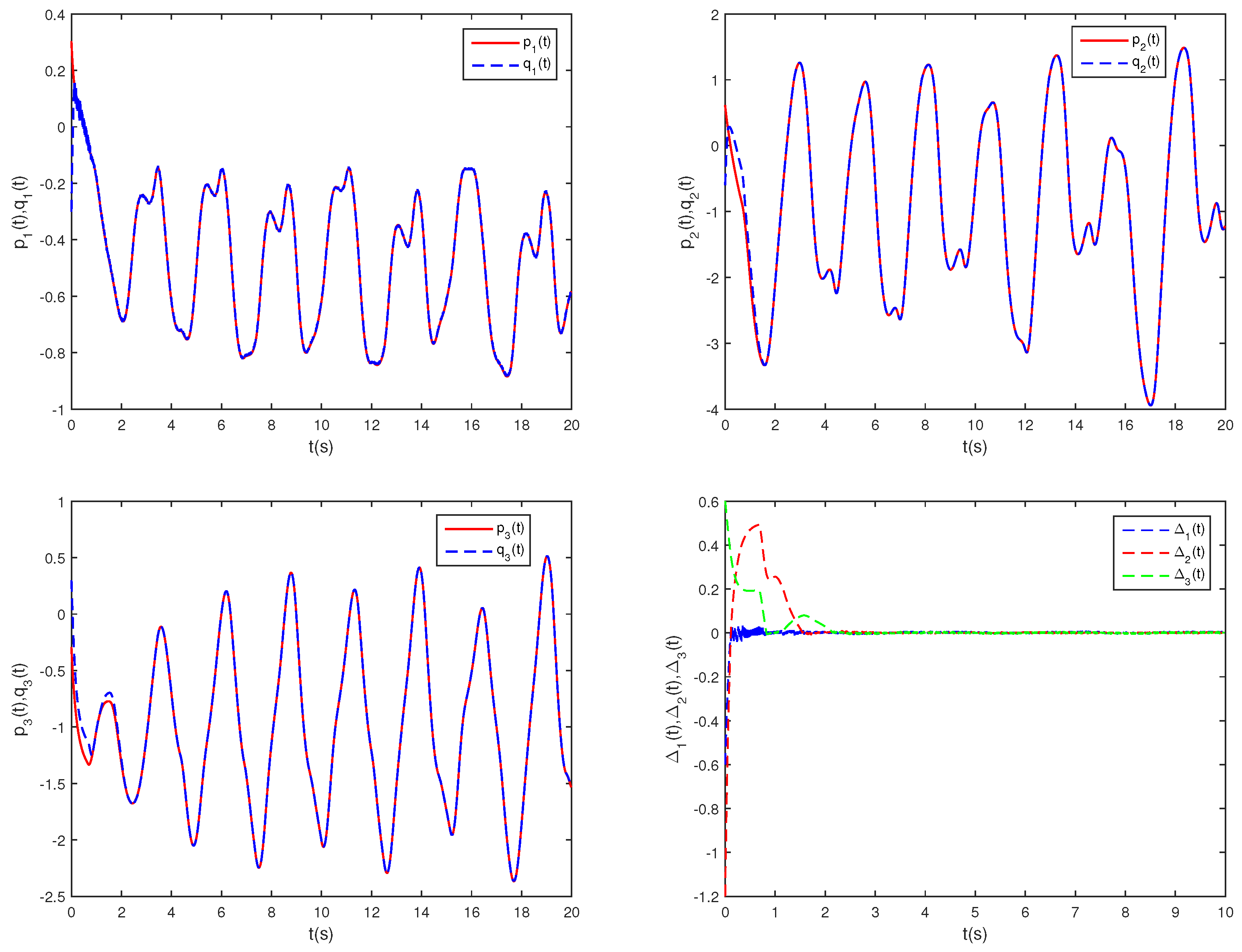
Example 1.
Consider the drive system:
The system parameter selection is as follows:
Let , , , , . . The initial values of system (29) are .
The response system is:
According to Theorem 1, control parameters should satisfy
Here, we choose
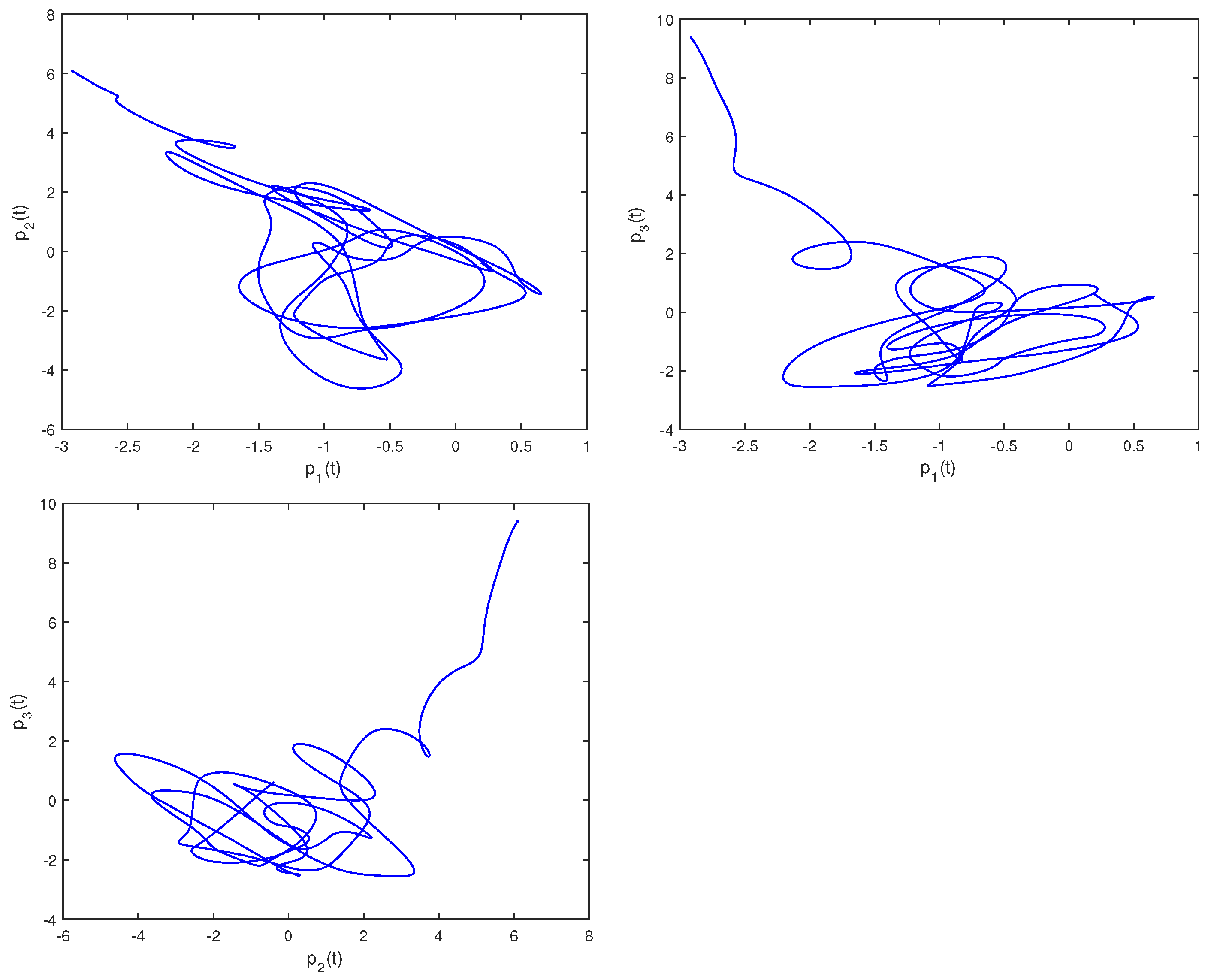
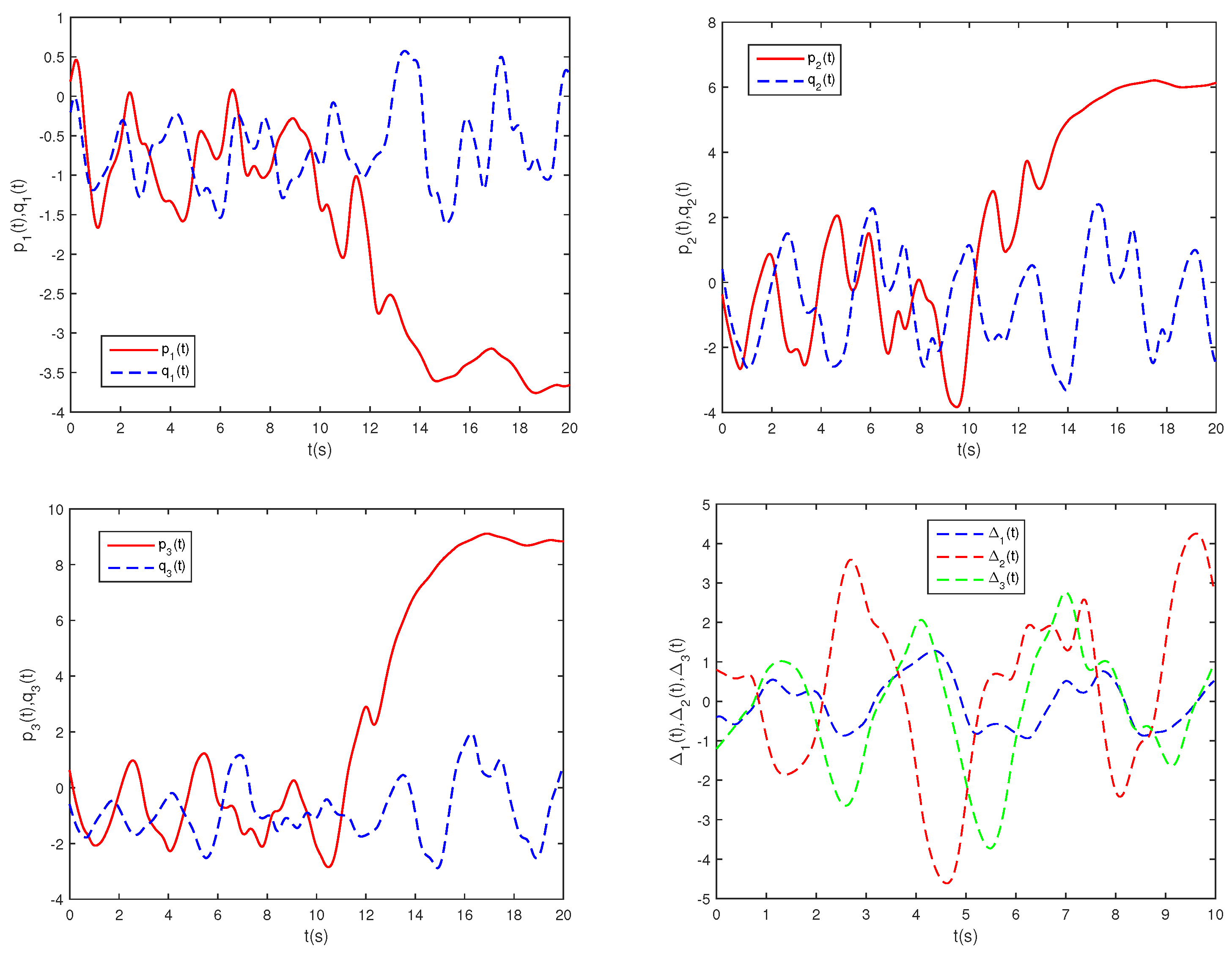
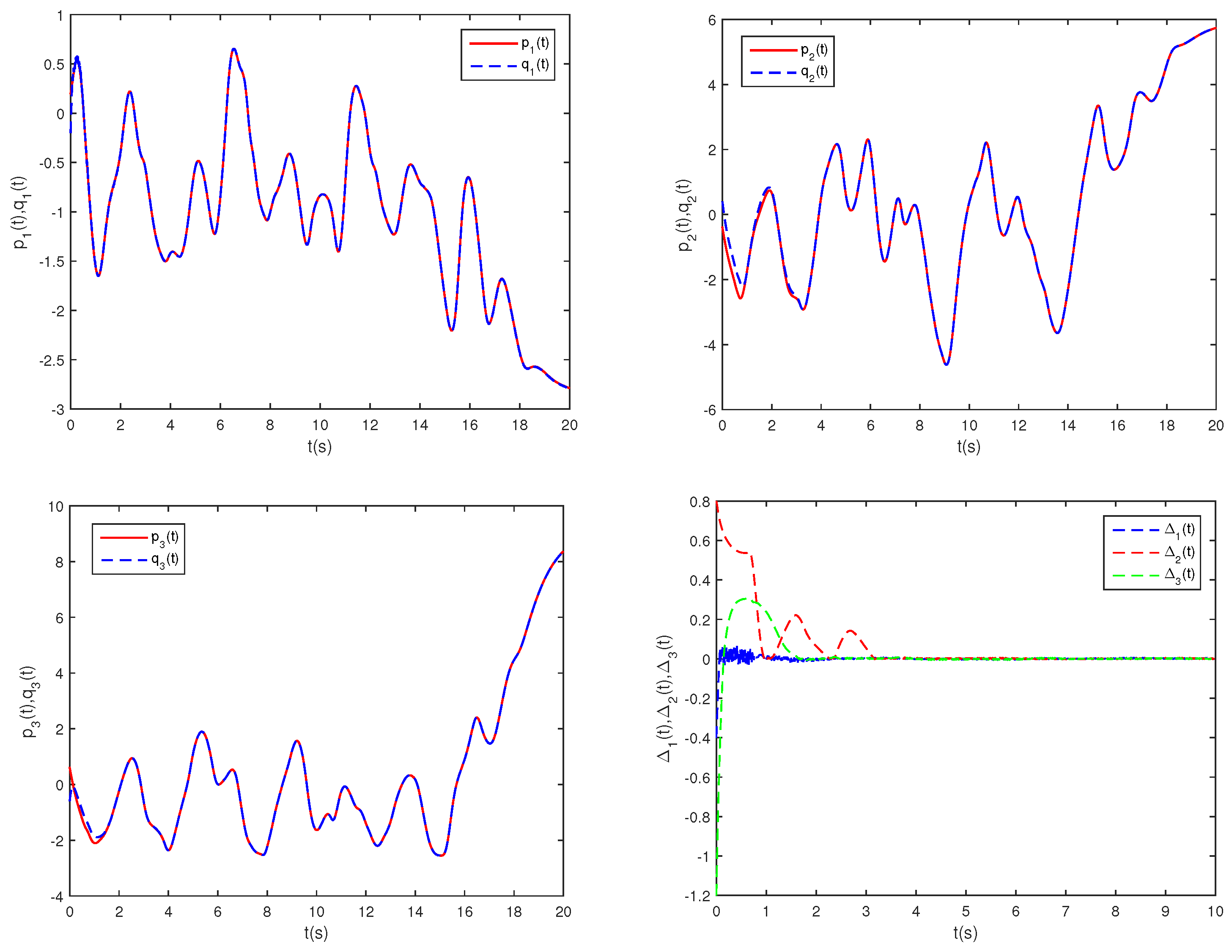
Figure 1 illustrates the phase trajectories of system (29) in two-dimensional state space without controller. Figure 2 show the state trajectories of systems (29) and (31) without controller. Figure 2 indicates that they have not reached synchronization without controller. Figure 3 show the state trajectories of systems (29) and (31) with controller. Figure 3 shows the state trajectories of the error system with controller. Figure 3 indicates that they can achieve synchronization within a finite time under this controller (16). Furthermore, according to Theorem 1, can be computed using Formula (18). This sufficiently confirms that Theorem 2 is effective.

Figure 1.
Phase trajectories of (29) in two–dimensional spaces.
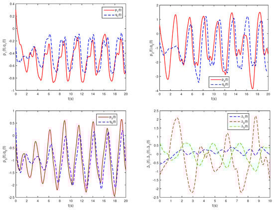
Figure 2.
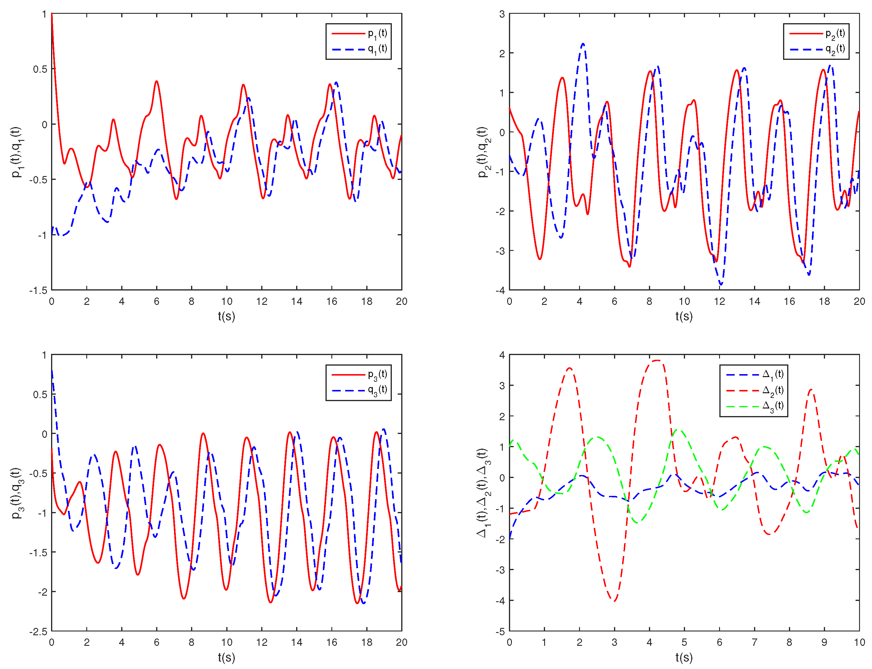
State trajectories of , , and without controller.
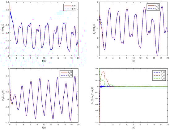
Figure 3.
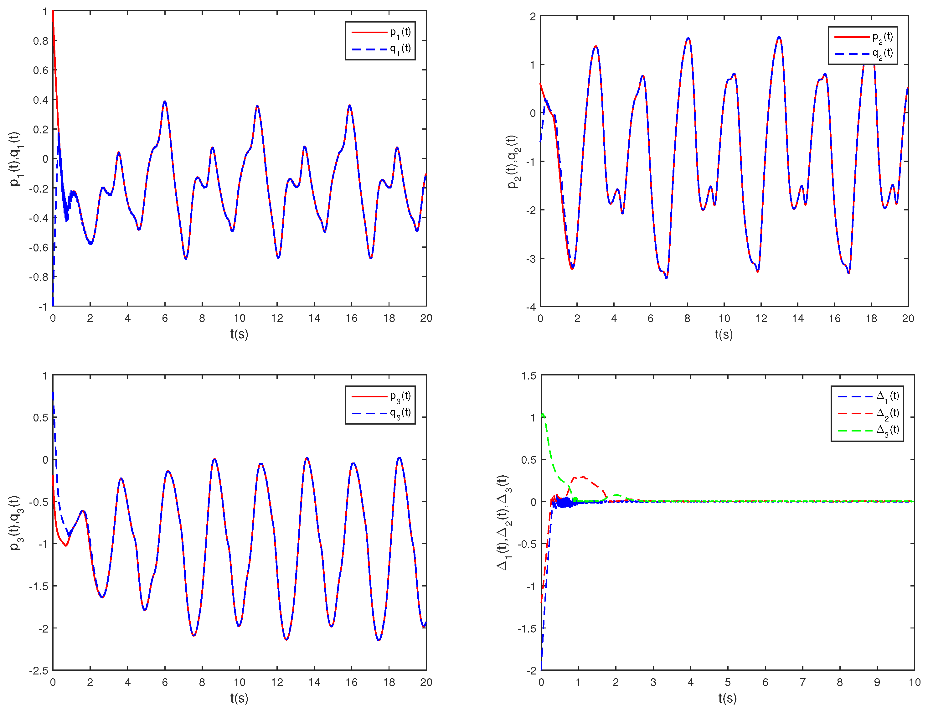
State trajectories of , , and with controller.
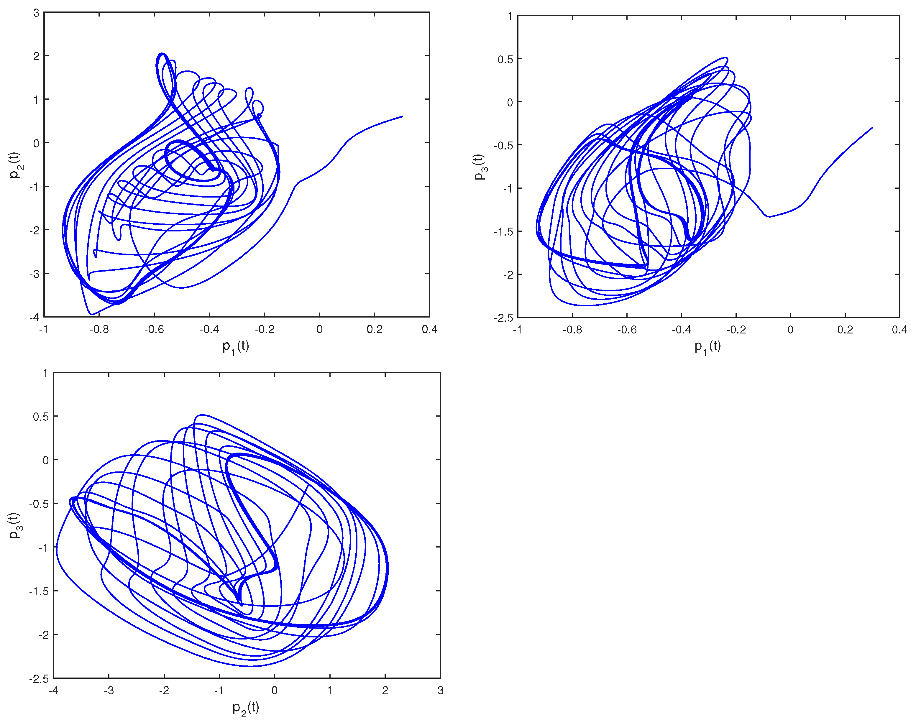
Example 2.
For system (29), the system parameter selection is as follows:
Let , , , , . . The initial values of system (29) are .
According to Theorem 2, control gains should satisfy
Here, we choose
Let , , .
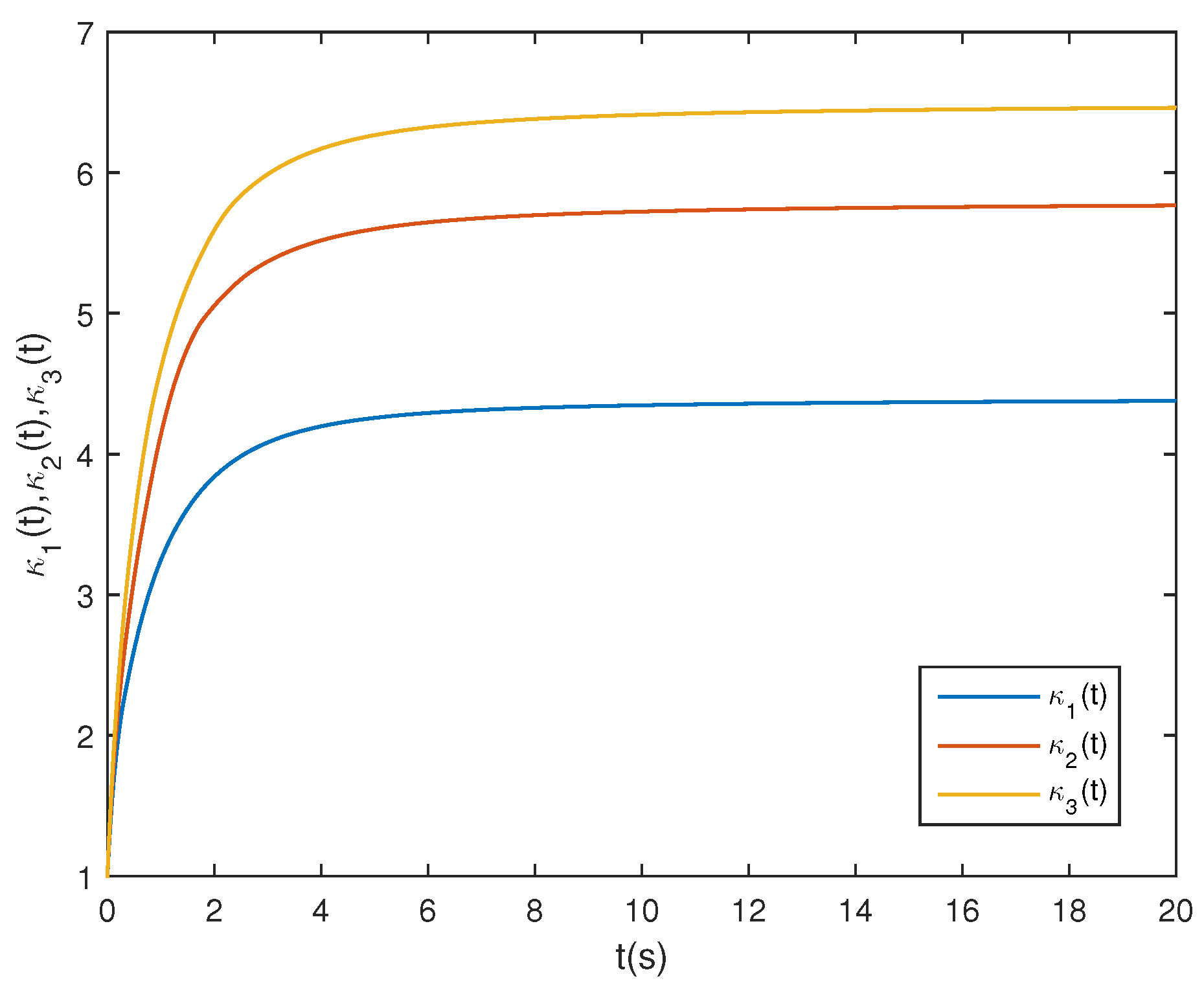
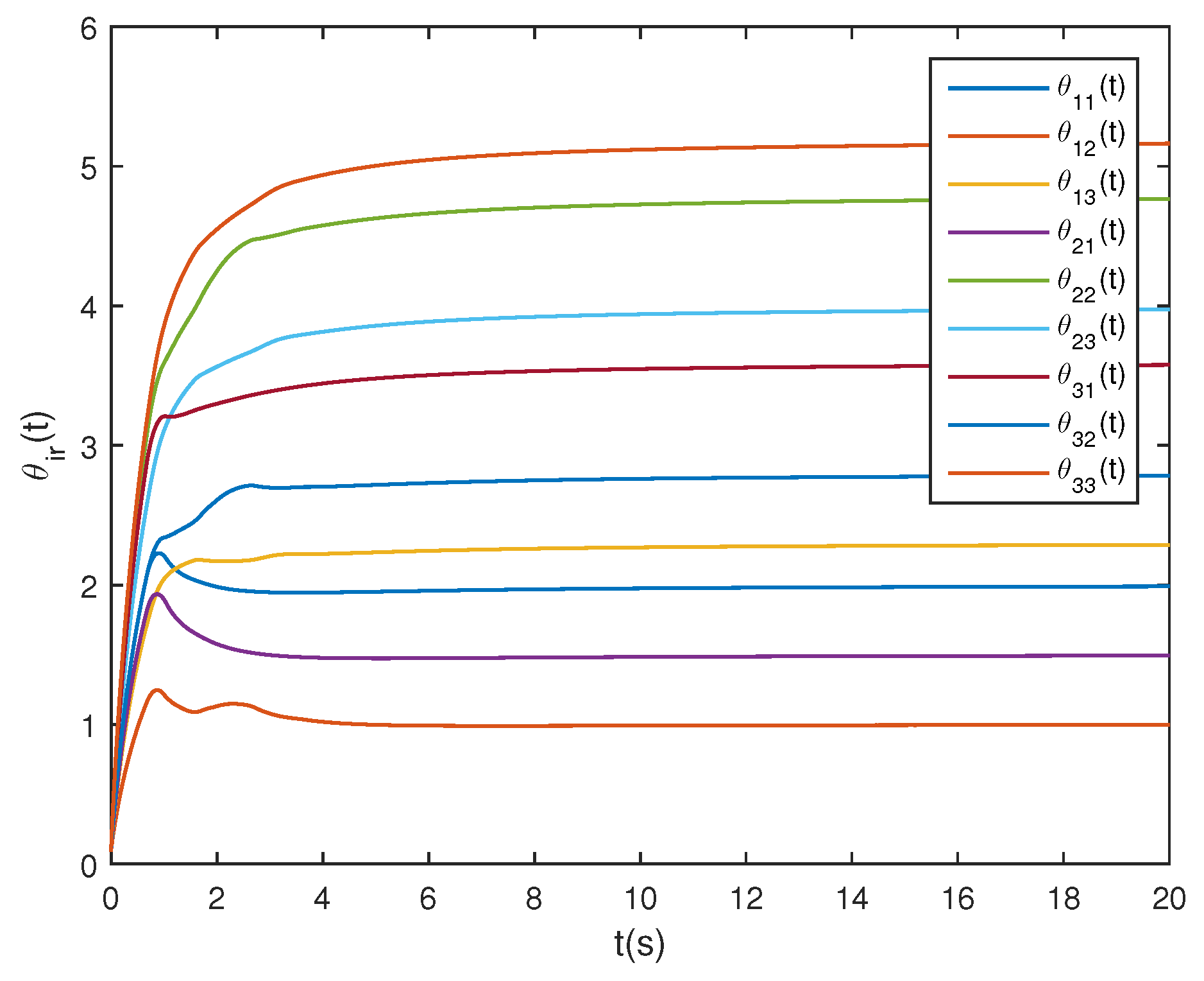
Figure 4 illustrates the phase trajectories of system (29) in two-dimensional state space without controller. Figure 5 show the state trajectories of systems (29) and (31) without controller. Figure 5 indicates that they have not reached synchronization without controller. Figure 6 show the state trajectories of systems (29) and (31) with controller. Figure 6 shows the state trajectories of the error system with controller. Figure 6 indicates that they can achieve synchronization within a finite time under this controller (17). Furthermore, according to Theorem 2, can be computed using Formula (18). Figure 7 and Figure 8 indicate the time response trajectory of the adaptive control gains and ,. This clearly indicates that the adaptive control gains , converge to some values within a finite time. This sufficiently confirms that Theorem 2 is effective.
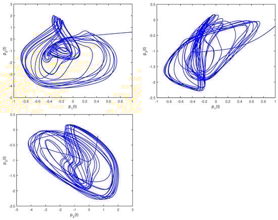
Figure 4.
Phase trajectories of (29) in two–dimensional spaces.
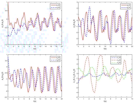
Figure 5.
State trajectories of , , and without controller.
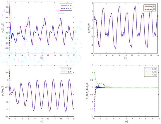
Figure 6.
State trajectoriesof , , and with controller.
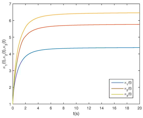
Figure 7.
State trajectories of control gains .
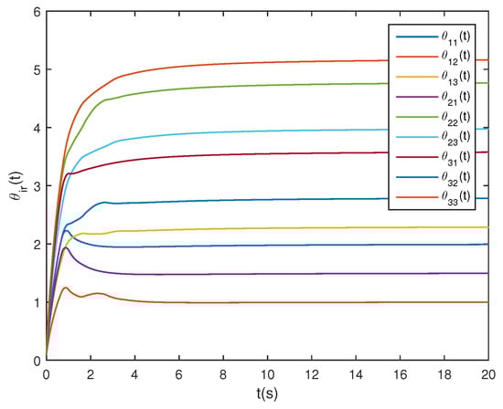
Figure 8.
State trajectories of control gains .
Example 3.
For system (29), the system parameter selection is as follows:
Let , , . . The initial values of system (29) are .
According to Theorem 3, control gains should satisfy
Here, we choose
Figure 9 illustrates the phase trajectories of system (29) in two-dimensional state space without controller. Figure 10 show the state trajectories of systems (29) and (31) without controller. Figure 10 indicates that they have not reached synchronization without controller. Figure 11 show the state trajectories of systems (29) and (31) with controller. Figure 11 shows the state trajectories of the error system with controller. Figure 11 indicates that they can achieve synchronization before a fixed time point under this controller (26). Furthermore, according to Theorem 3, can be computed using Formula (27). This sufficiently confirms that Theorem 3 is effective.
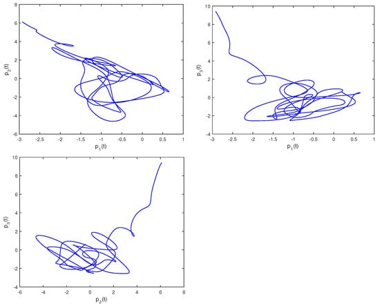
Figure 9.
Phase trajectories of (29) in two-dimensional spaces.
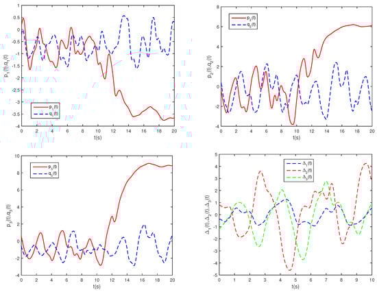
Figure 10.
State trajectories of , , and without controller.
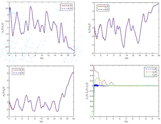
Figure 11.
State trajectories of , , and with controller.
6. Conclusions
This paper explores the finite-time adaptive synchronization and fixed-time synchronization of FMCNNs with TVD. Utilizing the properties and principles of fractional order, we introduce a novel lemma. Based on this lemma and various analysis techniques, we establish new criteria to guarantee FTAS and FDTS of FMCNNs with TVD through the implementation of a delay-dependent feedback controller and fractional-order adaptive controller. Additionally, we estimate the upper bound of the synchronization setting time. Finally, numerical simulations are conducted to confirm the validity of the finite-time and fixed-time stability theorems. The results of the numerical simulations substantiate the validity of the conclusions presented in this paper. In future work, based on the research results of this article, we will further study the synchronization problem of discrete-time FMCNNs with TVD.
Author Contributions
Conceptualization, methodology, writing—original draft preparation, Y.L. and Y.S.; writing—review and editing, numerical simulation, Y.L.; project administration, Y.S. All authors have read and agreed to the published version of the manuscript.
Funding
This work was partly supported by the Natural Science Foundation of Anhui Province (2008085MF200), the Program for Innovative Research Team in Universities of Anhui Province (2022AH010085), the University Natural Science Foundation of Anhui Province (KJ2021A0970), the National Natural Science Foundation of China (61403157), and the Research and Development Plan Project Foundation of Huainan (2021A248).
Data Availability Statement
The data presented in this study are available in the article.
Acknowledgments
The authors would like to thank the anonymous referees and reviewers for their helpful comments, which have significantly improved the quality of the presentation.
Conflicts of Interest
The authors declare no conflicts of interest.
References
- Yang, X.; Ho, D.W. Synchronization of delayed memristive neural networks: Robust analysis approach. IEEE Trans. Cybern. 2015, 46, 3377–3387. [Google Scholar] [CrossRef]
- Wen, S.; Zeng, Z.; Huang, T.; Zhang, Y. Exponential adaptive lag synchronization of memristive neural networks via fuzzy method and applications in pseudorandom number generators. IEEE Trans. Fuzzy Syst. 2013, 22, 1704–1713. [Google Scholar] [CrossRef]
- Hu, X.; Feng, G.; Duan, S.; Liu, L. A memristive multilayer cellular neural network with applications to image processing. IEEE Trans. Neural Netw. Learn. Syst. 2016, 28, 1889–1901. [Google Scholar] [CrossRef]
- Chua, L. Memristor-the missing circuit element. IEEE Trans. Circuit Theory 1971, 18, 507–519. [Google Scholar] [CrossRef]
- Ali, M.S.; Hymavathi, M.; Senan, S.; Shekher, V.; Arik, S. Global asymptotic synchronization of impulsive fractional-order complex-valued memristor-based neural networks with time varying delays. Commun. Nonlinear Sci. Numer. Simul. 2019, 78, 104869. [Google Scholar]
- Li, N.; Zheng, W.X. Synchronization criteria for inertial memristor-based neural networks with linear coupling. Neural Netw. 2018, 106, 260–270. [Google Scholar] [CrossRef]
- Wu, K.; Jian, J. Non-reduced order strategies for global dissipativity of memristive neutral-type inertial neural networks with mixed time-varying delays. Neurocomputing 2021, 436, 174–183. [Google Scholar] [CrossRef]
- Zhang, T.; Jian, J. New results on synchronization for second-order fuzzy memristive neural networks with time-varying and infinite distributed delays. Knowl.-Based Syst. 2021, 230, 107397. [Google Scholar] [CrossRef]
- Sun, Y.; Liu, Y.; Liu, L. Asymptotic and finite-time synchronization of fractional-order memristor-based inertial neural networks with time-varying delay. Fractal Fract. 2022, 6, 350. [Google Scholar] [CrossRef]
- Zhang, X.; Jiang, W. Construction of flux-controlled memristor and circuit simulation based on smooth cellular neural networks module. IET Circuits Devices Syst. 2018, 12, 263–270. [Google Scholar] [CrossRef]
- Ascoli, A.; Messaris, I.; Tetzlaff, R.; Chua, L.O. Theoretical foundations of memristor cellular nonlinear networks: Stability analysis with dynamic memristors. IEEE Trans. Circuits Syst. I Regul. Pap. 2019, 67, 1389–1401. [Google Scholar] [CrossRef]
- Song, C.; Cao, J. Dynamics in fractional-order neural networks. Neurocomputing 2014, 142, 494–498. [Google Scholar] [CrossRef]
- Wang, H.; Yu, Y.; Wen, G. Stability analysis of fractional-order Hopfield neural networks with time delays. Neural Netw. 2014, 55, 98–109. [Google Scholar] [CrossRef]
- Ma, Z.; Ma, H. Adaptive fuzzy backstepping dynamic surface control of strict-feedback fractional-order uncertain nonlinear systems. IEEE Trans. Fuzzy Syst. 2020, 28, 122–133. [Google Scholar] [CrossRef]
- Zhang, Q.; Lu, J. Bounded real lemmas for singular fractional-order systems: The 1 < α < 2 case. IEEE Trans. Circuits Syst. II Express Briefs 2021, 68, 732–736. [Google Scholar]
- Shafiya, M.; Nagamani, G.; Dafik, D. Global synchronization of uncertain fractional-order BAM neural networks with time delay via improved fractional-order integral inequality. Math. Comput. Simul. 2022, 191, 168–186. [Google Scholar] [CrossRef]
- Yan, S.; Gu, Z.; Nguang, S. Memory-event-triggered H∞ output control of neural networks with mixed delays. IEEE Trans. Neural Netw. Learn. Syst. 2022, 33, 6905–6915. [Google Scholar] [CrossRef] [PubMed]
- Jian, J.; Duan, L. Finite-time synchronization for fuzzy neutral-type inertial neural networks with time-varying coefficients and proportional delays. Fuzzy Sets Syst. 2020, 381, 51–67. [Google Scholar] [CrossRef]
- Li, H.L.; Zhang, L.; Hu, C.; Jiang, H.; Cao, J. Global Mittag-Leffler synchronization of fractional-order delayed quaternion-valued neural networks: Direct quaternion approach. Appl. Math. Comput. 2020, 373, 125020. [Google Scholar] [CrossRef]
- Zhang, H.; Cheng, J.; Zhang, H.; Zhang, W.; Cao, J. Quasi-uniform synchronization of Caputo type fractional neural networks with leakage and discrete delays. Chaos Solitons Fractals 2021, 152, 111432. [Google Scholar] [CrossRef]
- Tong, D.; Zhang, L.; Zhou, W.; Zhou, J.; Xu, Y. Asymptotical synchronization for delayed stochastic neural networks with uncertainty via adaptive control. Int. J. Control Autom. Syst. 2016, 14, 706–712. [Google Scholar] [CrossRef]
- Xiong, X.; Zhang, Z. Asymptotic synchronization of conformable fractional-order neural networks by L’Hopital’s rule. Chaos Solitons Fractals 2023, 173, 113665. [Google Scholar] [CrossRef]
- Guo, Z.; Gong, S.; Yang, S.; Huang, T. Global exponential synchronization of multiple coupled inertial memristive neural networks with time-varying delay via nonlinear coupling. Neural Netw. 2018, 108, 260–271. [Google Scholar] [CrossRef]
- Zhang, T.; Jian, J. Quantized intermittent control tactics for exponential synchronization of quaternion-valued memristive delayed neural networks. ISA Trans. 2022, 126, 288–299. [Google Scholar] [CrossRef] [PubMed]
- Zheng, C.; Cao, J. Robust synchronization of coupled neural networks with mixed delays and uncertain parameters by intermittent pinning control. Neurocomputing 2014, 141, 153–159. [Google Scholar] [CrossRef]
- Duan, L.; Wei, H.; Huang, L. Finite-time synchronization of delayed fuzzy cellular neural networks with discontinuous activations. Fuzzy Sets Syst. 2019, 361, 56–70. [Google Scholar] [CrossRef]
- Li, H.L.; Cao, J.; Jiang, H.; Alsaedi, A. Graph theory-based finite-time synchronization of fractional-order complex dynamical networks. J. Frankl. Inst. 2018, 355, 5771–5789. [Google Scholar] [CrossRef]
- Lu, J.; Guo, Y.; Ji, Y.; Fan, S. Finite-time synchronization for different dimensional fractional-order complex dynamical networks. Chaos Solitons Fractals 2020, 130, 109433. [Google Scholar] [CrossRef]
- Shanmugam, S.; Narayanan, G.; Rajagopal, K.; Ali, M.S. Finite-time synchronization of complex-valued neural networks with reaction-diffusion terms: An adaptive intermittent control approach. Neural Comput. Appl. 2024, 36, 7389–7404. [Google Scholar] [CrossRef]
- He, X.; Wang, Y.; Li, T.; Kang, R.; Zhao, Y. Novel Controller Design for Finite-Time Synchronization of Fractional-Order Nonidentical Complex Dynamical Networks under Uncertain Parameters. Fractal Fract. 2024, 8, 155. [Google Scholar] [CrossRef]
- Xiao, J.; Wu, L.; Wu, A.; Zeng, Z.; Zhang, Z. Novel controller design for finite-time synchronization of fractional-order memristive neural networks. Neurocomputing 2022, 512, 494–502. [Google Scholar] [CrossRef]
- Duan, L.; Li, J. Fixed-time synchronization of fuzzy neutral-type BAM memristive inertial neural networks with proportional delays. Inf. Sci. 2021, 576, 522–541. [Google Scholar] [CrossRef]
- Polyakov, A. Nonlinear feedback design for fixed-time stabilization of linear control systems. IEEE Trans. Autom. Control 2011, 57, 2106–2110. [Google Scholar] [CrossRef]
- Cheng, Y.; Hu, T.; Xu, W.; Zhang, X.; Zhong, S. Fixed-time synchronization of fractional-order complex-valued neural networks with time-varying delay via sliding mode control. Neurocomputing 2022, 505, 339–352. [Google Scholar] [CrossRef]
- Sun, Y.; Liu, Y. Fixed-time synchronization of delayed fractional-order memristor-based fuzzy cellular neural networks. IEEE Access 2020, 8, 165951–165962. [Google Scholar] [CrossRef]
- Li, X.; Fang, J.A.; Zhang, W.; Li, H. Finite-time synchronization of fractional-order memristive recurrent neural networks with discontinuous activation functions. Neurocomputing 2018, 316, 284–293. [Google Scholar] [CrossRef]
- Li, J.; Jiang, H.; Hu, C.; Alsaedi, A. Finite/fixed-time synchronization control of coupled memristive neural networks. J. Frankl. Inst. 2019, 356, 9928–9952. [Google Scholar] [CrossRef]
- Li, X.; Zhang, W.; Fang, J. Finite-time synchronization of memristive neural networks with discontinuous activation functions and mixed time-varying delays. Neurocomputing 2019, 340, 99–109. [Google Scholar] [CrossRef]
- Zhang, Y.; Deng, S. Finite-time projective synchronization of fractional-order complex-value d memristor-base d neural networks with delay. Chaos Solitons Fractals 2019, 128, 176–190. [Google Scholar] [CrossRef]
- Guo, Z. Finite-time synchronization of inertial memristive neural networks with time delay via delay-dependent control. Neurocomputing 2018, 293, 100–107. [Google Scholar] [CrossRef]
- Wei, F.; Chen, G.; Zeng, Z.; Gunasekaran, N. Finite/fixed-time synchronization of inertial memristive neural networks by interval matrix method for secure communication. Neural Netw. 2023, 167, 168–182. [Google Scholar] [CrossRef] [PubMed]
- Gong, S.; Guo, Z.; Wen, S. Finite-time synchronization of TS fuzzy memristive neural networks with time delay. Fuzzy Sets Syst. 2023, 459, 67–81. [Google Scholar] [CrossRef]
- Zhao, F.; Jian, J.; Wang, B. Finite-time synchronization of fractional-order delayed memristive fuzzy neural networks. Fuzzy Sets Syst. 2023, 467, 108578. [Google Scholar] [CrossRef]
- Arslan, E.; Narayanan, G.; Ali, M.S.; Arik, S.; Saroha, S. Controller design for finite-time and fixed-time stabilization of fractional-order memristive complex-valued BAM neural networks with uncertain parameters and time-varying delays. Neural Netw. 2020, 130, 60–74. [Google Scholar] [CrossRef] [PubMed]
- Wang, W.; Jia, X.; Wang, Z.; Luo, X.; Li, L.; Kurths, J.; Yuan, M. Fixed-time synchronization of fractional order memristive MAM neural networks by sliding mode control. Neurocomputing 2020, 401, 364–376. [Google Scholar] [CrossRef]
- Xiao, J.; Hu, Y.; Zeng, Z.; Wu, A.; Wen, S. Fixed/predefined-time synchronization of memristive neural networks based on state variable index coefficient. Neurocomputing 2023, 560, 126849. [Google Scholar] [CrossRef]
- Wang, D.; Li, L. Fixed-time synchronization of delayed memristive neural networks with impulsive effects via novel fixed-time stability theorem. Neural Netw. 2023, 163, 75–85. [Google Scholar] [CrossRef]
- Podlubny, I. Fractional Differential Equations; Academic Press: New York, NY, USA, 1999. [Google Scholar]
- Lakshmikantham, V.; Vatsala, A. Basic theory of fractional differential equations. Nonlinear Anal. 2008, 69, 2677–2682. [Google Scholar] [CrossRef]
- Zhang, S.; Yu, Y.; Wang, H. Mittag-Leffler stability of fractional-order hopfield neural networks. Nonlin. Anal. Hybrid Syst. 2015, 16, 104–121. [Google Scholar] [CrossRef]
- Yu, J.; Hu, C.; Jiang, H. Corrigendum to Projective synchronization for fractional neural networks. Neural Netw. 2015, 67, 152–154. [Google Scholar] [CrossRef]
- Kong, F.; Zhu, Q.; Sakthivel, R. Finite-time and fixed-time synchronization analysis of fuzzy Cohen-Grossberg neural networks with piecewise activations and parameter uncertainties. Eur. J. Control 2020, 56, 179–190. [Google Scholar] [CrossRef]


Disclaimer/Publisher’s Note: The statements, opinions and data contained in all publications are solely those of the individual author(s) and contributor(s) and not of MDPI and/or the editor(s). MDPI and/or the editor(s) disclaim responsibility for any injury to people or property resulting from any ideas, methods, instructions or products referred to in the content. |
© 2024 by the authors. Licensee MDPI, Basel, Switzerland. This article is an open access article distributed under the terms and conditions of the Creative Commons Attribution (CC BY) license (https://creativecommons.org/licenses/by/4.0/).