1. Introduction
Material mechanical properties play a fundamental role in various areas, such as design specifications, manufacturing processes, operational methods, and failure analysis. Conventional experiments are frequently employed to ascertain the mechanical properties of materials. Extensive testing can be resource-intensive and non-directional, which is frequently unavoidable in the search for innovative materials with improved performance. Moreover, traditional methods struggle to keep pace with the modern industrial need for high quality, rapid production cycles, and cost efficiency. Therefore, there is a growing necessity to swiftly and accurately predict the mechanical properties of materials.
Predicting material performance presents challenges. Factors like chemical composition, element content, manufacturing processes, and operating temperatures intricately influence material behavior, creating a complex nonlinear system that is challenging to decipher. Although data form the backbone of material performance prediction, the time-consuming nature of material testing sometimes results in small datasets. Effectively identifying the nonlinear system under limited sample conditions becomes crucial for ensuring the reliability of material attribute predictions.
In response to these issues, scientists have proposed various predictive methods, including empirical formulations [
1,
2], linear regression analysis [
3,
4], finite element analysis (FEA) [
5], and Monte Carlo methods [
6,
7,
8,
9]. These methods are predominantly empirical and statistical in nature. However, the practical implementation of these methods is often hindered by the inherent difficulties in capturing nonlinear correlations within the data, leading to reduced prediction accuracy and limited generalizability. Mechanism modeling has emerged as an alternative approach for predicting the mechanical properties of materials. Nonetheless, the complexity of these mechanisms, which are contingent upon production and manufacturing processes, restrict their applicability. For instance, traditional metallurgical mechanism models, while effective in representing most processing procedures, are structurally complex, computationally intensive, and require a deep understanding of specific metallurgical processes as a prerequisite [
10].
Researchers have increasingly focused on utilizing machine learning methods to predict material performance, leveraging their capacity to extract high-dimensional features from raw data [
11,
12,
13,
14,
15]. By effectively capturing the nonlinear relationships between material parameters and mechanical properties, machine learning models offer valuable insights into the complex interplay, thus guiding experimental efforts [
16]. Ke Duan et al. [
17] developed a model that integrates molecular dynamics simulations, particle swarm optimization (PSO), and artificial neural networks to determine the coarse granulation of cross-linked epoxy resins. Similarly, Georgios Konstantopoulos et al. [
18] introduced a machine learning model to elucidate the structure–property relationship in carbon fiber-reinforced polymer composites (CFRPs), comparing the classification performance of neural networks, decision trees, and support vector machines. In another study, Yupeng Diao [
19] devised a predictive model for steel corrosion by translating chemical composition into physical characteristics. Meanwhile, Changsheng Wang [
20] employed a machine learning system for the design of alloy material compositions, thereby expediting the material development process. M.Z. Naser [
21] put forth an analytical model based on symbolic regression and genetic algorithms (GAs) to forecast the behavior of concrete structures under high-temperature conditions. Additional research endeavors encompassed the prediction of solute behaviors in ductile magnesium alloys [
22], residual stress estimation in aluminum plates using the K-Nearest Neighbors (KNN) algorithm [
23], and the evaluation of glass fiber orientation through a convolutional neural network and inertial tensor analysis [
24].
From the above research, it can be observed that current machine learning used for material performance prediction can mainly be divided into artificial neural networks, backpropagation networks, tree models and their variations, and deep neural networks. The accuracy of regression models based on artificial neural networks highly depends on the quality and quantity of the input data. If the dataset is insufficient or contains noise, the predictive ability of the model is likely to be affected. Although training neural network models with backpropagation can help the model converge quickly, its performance is still influenced by multiple hyperparameters, such as the learning rate, hidden layer, and number of neurons, which are often set empirically.
Subsequently, prediction methods based on tree models, such as random forests, have shown good performance, but they also require a large amount of parameter tuning and computational resources, especially as the dataset size increases, as the model can become time-consuming. Moreover, if the model overfits the training data, it may perform poorly on the test data.
Some deep learning models may perform well in predicting the performance of specific types of metals, but for different types of alloys, they may require readjustments to provide satisfactory predictive performance. For example, deep neural networks usually require a substantial number of computational resources and time for training, which may limit their feasibility in practical applications. Lastly, in many cases, the datasets for metals are small, which requires the developed predictive models to quickly learn the nonlinear relationship between metal elements and mechanical performance.
Consequently, the development of efficient machine learning models capable of predicting the mechanical properties of materials holds paramount importance while also furnishing valuable insights for the advancement of new materials. For instance, comprehending the intricate interrelationships among process parameters, structural configurations, and mechanical properties of alloys is indispensable for conducting retrospective analyses and identifying the optimal process parameters [
25]. Low-alloy steel holds significant value in various industries due to its consistent quality, excellent corrosion resistance, remarkable technological properties, and high recovery rate. These types of steel find applications in engineering plants, aircraft bodies, automobiles, ships, buildings, and bridges. The mechanical characteristics of alloy steel are predominantly governed by their chemical composition and manufacturing process [
26,
27]. However, the rolling process of alloy steel presents a complex and nonlinear system, posing significant challenges in mathematically expressing these relationships [
28]. Studies have indicated that the microstructure of alloys, influenced by their chemical composition, manufacturing method, and operating temperature, plays a crucial role in determining their properties [
29,
30]. Consequently, a machine learning-based model leveraging elemental composition and microstructure can be developed to forecast the mechanical properties of low-alloy steel.
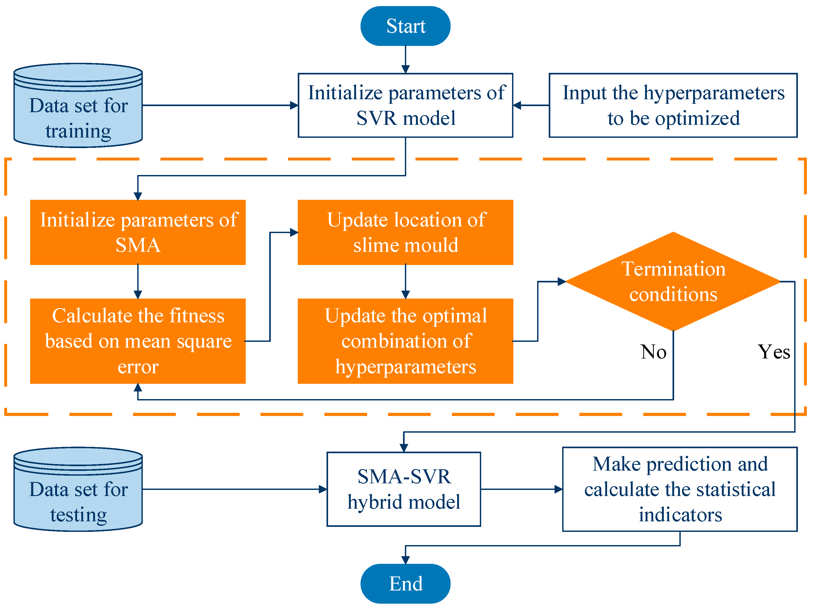
In this paper, a hybrid framework utilizing support vector regression (SVR) optimized by the Slime Mould Algorithm (SMA) is proposed to predict the mechanical properties of low-alloy steel. SVR is well-suited to address challenges associated with high dimensionality, small sample size, and nonlinearity, while SMA is adept at searching for and optimizing the penalty factor and kernel parameter of SVR to boost prediction accuracy and robustness. The study employs data on low-alloy steel from the NIMS Materials Database and data from material tests conducted on a universal testing machine (UTM). The target is to predict two key mechanical parameters: tensile strength and 0.2% proof stress. The model’s predictive prowess was assessed using four statistical criteria—Mean Absolute Error (MAE), R
2 (R-Squared), computational time, and Root Mean Square Error (RMSE). Furthermore, three popular hybrid models optimized through metaheuristics were selected and compared with SMA-SVR. These models included SVR optimized by Grey Wolf Optimizer (GWO-SVR), Back Propagation optimized by particle swarm optimization (PSO-BP), and the Elman recurrent neural network optimized by the Sparrow Search Algorithm (SSA-Elman), all of which have exhibited promising performance in engineering and materials science studies [
31,
32,
33,
34,
35,
36,
37]. The parameters of the respective models were fine-tuned using metaheuristic algorithms. The discussion delves into the experimental findings of SMA-SVR, along with its comparative analysis with GWO-SVR, PSO-BP, and SSA-Elman.
The novelty of this study can be mainly summarized in the following points:
Firstly, this work combines SMA with SVR to optimize the key hyperparameters, which is not commonly seen in previous studies on predicting the mechanical properties of materials in materials science. The proposed model is specifically applied and discussed in the domain of predicting the mechanical properties of low-alloy steel, which is a practical contribution to the interdisciplinary field of materials science and artificial intelligence.
Secondly, the established hybrid model provides comprehensive experimental validation by comparing it with different popular models, thereby analyzing the effectiveness and unique features of the proposed method.
Lastly, the model training and validation are conducted using the data from both the NIMS database and UTM testing. By incorporating publicly available data for testing the model performance and utilizing small-sample datasets for validation, the practicality and credibility of the research are enhanced.
The subsequent sections of this paper include the following: a detailed exploration of the modeling process and evaluation metrics in
Section 2, an investigation and discourse on the prediction accuracy and efficacy of hybrid models utilizing the NIMS database in
Section 3, prediction experiments employing material test data from the UTM in
Section 4, and a conclusive summary accompanied by insights into future research avenues in
Section 5.
3. Test Cases and Discussion Based on NIMS Database Data
3.1. The Source and Introduction of the Data from NIMS Database
In
Section 3.1,
Section 3.2 and
Section 3.3, a dataset of low-alloy steel was utilized. It was sourced from the Materials Database of the National Institute for Materials Science [
43] (
https://cds.nims.go.jp/). However, the data available in the NIMS Materials Database were solely provided in PDF format. Thus, an open-source OCR tool (PaddleOCR) was employed to structure the data on low-alloy steel into a tabular format. While the use of an OCR tool proves to be a convenient method for converting PDF data into tabular form, it may introduce certain limitations and biases. Following the identification and merging process checks to ensure the consistency between the original and identified data were also conducted. Subsequently, a dataset consisting of 914 samples, each encompassing 16 features, was compiled. These features included 11 elements of the content of low-alloy steel, 1 facet of temperature information, and 4 attributes concerning the mechanical properties of materials. For a detailed overview of the features, please refer to
Table 2.
3.2. Tests and Discussion of Tensile Strength Prediction
Tensile strength stands out as a pivotal variable extensively utilized in design, structural analysis, manufacturing quality management, failure analysis, and other relevant fields. Hence, tensile strength was chosen as the target variable for prediction in this section. The content of elements and temperature of materials, as outlined in
Table 2, were selected as the input features for model training. The data were partitioned into training and test sets at a ratio of 7:3. Specifically, 640 rows of data were randomly assigned as the training data input for each modeling iteration, while the remaining 274 rows were earmarked for the test set.
The performance of these hybrid models (SMA-SVR, GWO-SVR, PSO-BP, and SSA-Elman) was assessed. All experiments were carried out on a single computer equipped with an Intel Core i7-11800H processor, Samsung DDR4 3200 MHz 16 GB memory, and NVIDIA GeForce RTX 3060 6 GB graphics card. To gauge the robustness of each hybrid model, the testing process was conducted ten times and documented the average values (MEAN) and standard deviations (STDs) of the results, which are detailed in
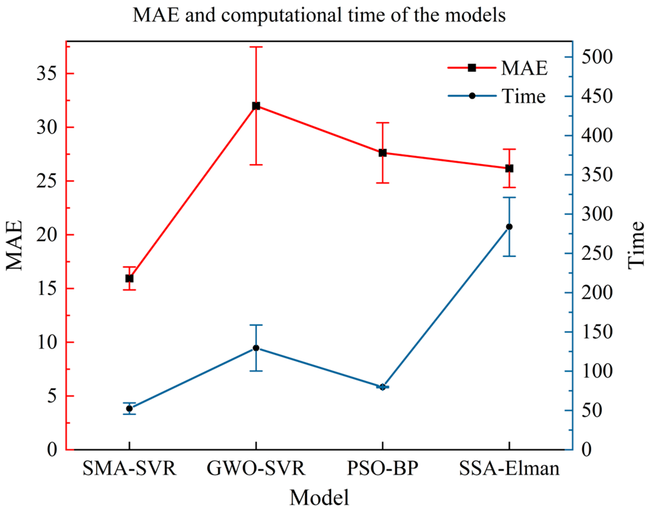
Table 3. To present the test results more intuitively, a dual
Y-axis line chart with error intervals was created, as shown in
Figure 2. The horizontal axis represents different hybrid models; the left vertical axis corresponds to the MAE of the test results, and the right vertical axis represents the computational time of these models. The legend indicates MAE and time (marked in red and blue, respectively), corresponding to the left and right vertical axes.
The performance of the four hybrid models is compared using different evaluation metrics. The results indicate that the MAE of SMA-SVR is significantly smaller than that of the other three models, with SSA-Elman achieving the lowest MAE of 26.1757. Notably, the MAE of SMA-SVR is 39.12% smaller than that of SSA-Elman. When analyzing RMSE, SMA-SVR demonstrates superior performance compared to PSO-BP, SSA-Elman, and GWO-SVR, in that order. Specifically, the discrepancy between the predicted and actual values is the smallest for SMA-SVR, while GWO-SVR exhibits the largest RMSE among them.
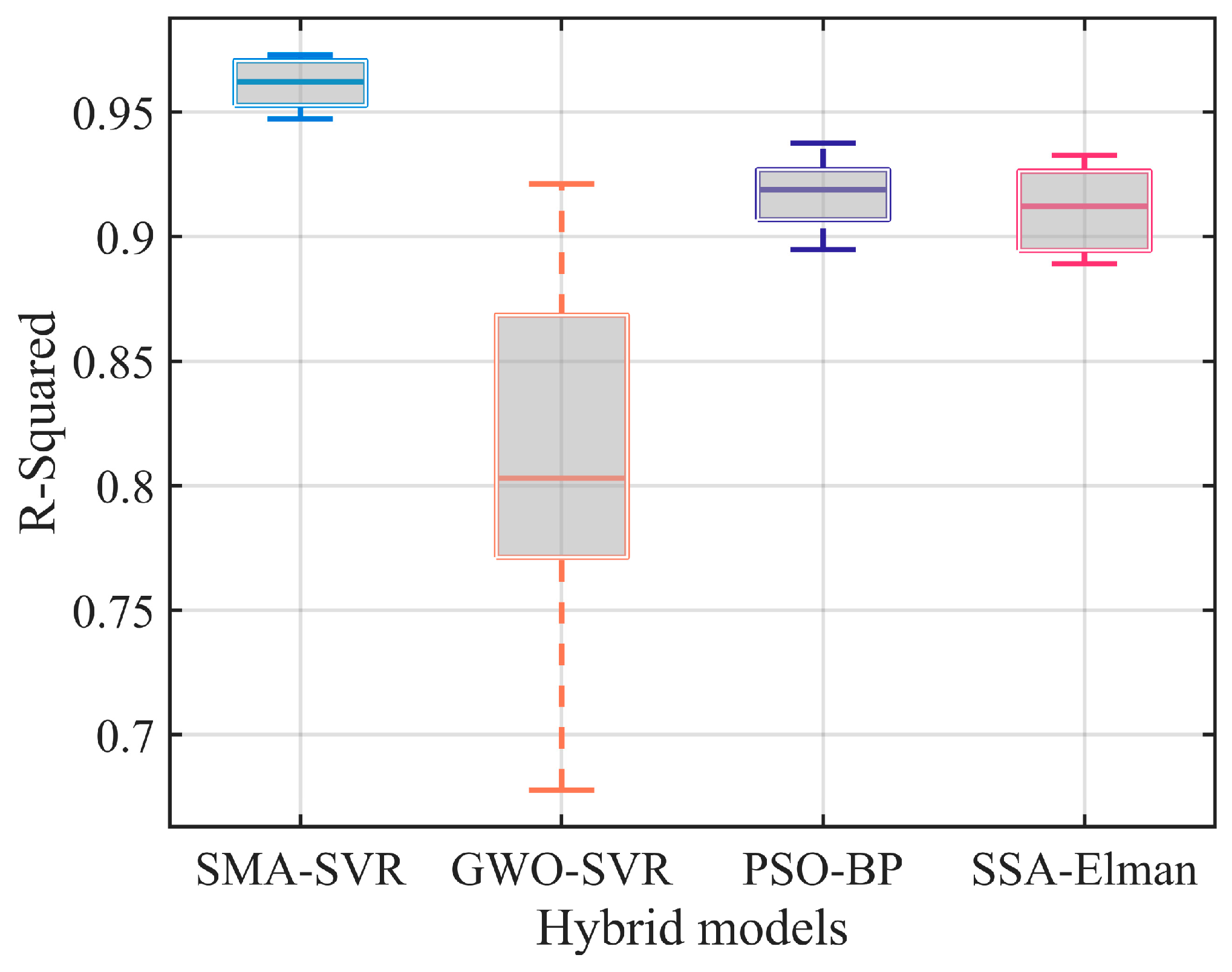
In the evaluation of the R2, which indicates the goodness of fit of the regression model, SMA-SVR stands out with an R2 value of 0.9602. The low standard deviation of R2 at 0.0108 suggests that the predictions made by SMA-SVR are highly stable, with minimal data dispersion. It is noteworthy that a significantly shorter average computational time was required by SMA-SVR compared to GWO-SVR, PSO-BP, and SSA-Elman. In particular, the computational time of SMA-SVR is 81.53%, which is less than that of SSA-Elman.
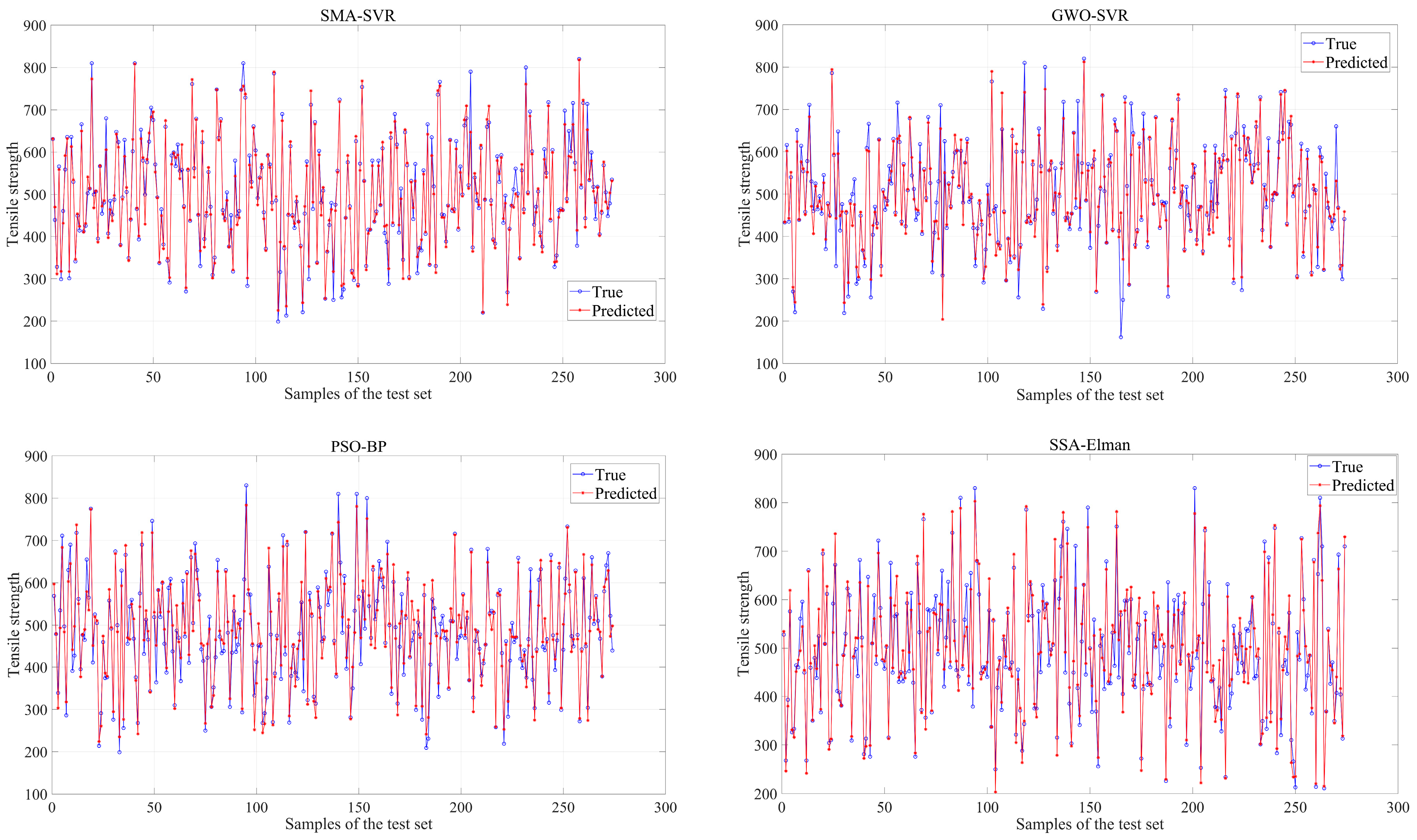
The analyses demonstrate that the predictive performance of SMA-SVR outperforms the other three hybrid models significantly. To further evaluate the models, the best prediction results from these tests are recorded. A comparison chart is designed to display the actual and predicted values of the test set for each model, as depicted in
Figure 3. Moreover, a box plot of R
2 values is constructed to facilitate visual comparison of their prediction accuracy, as illustrated in
Figure 4.
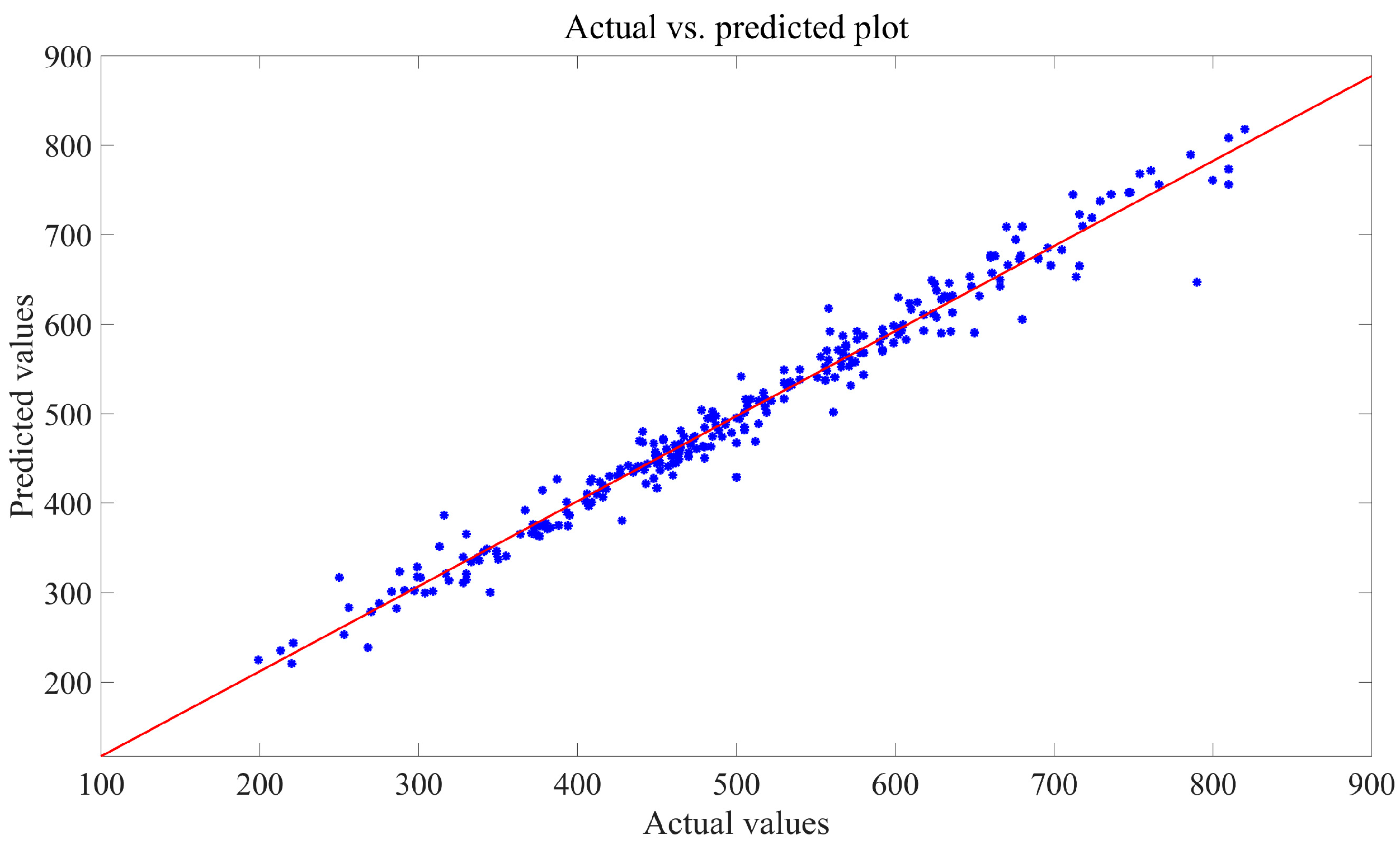
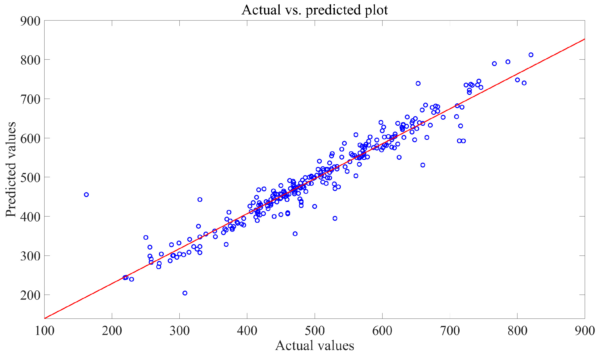
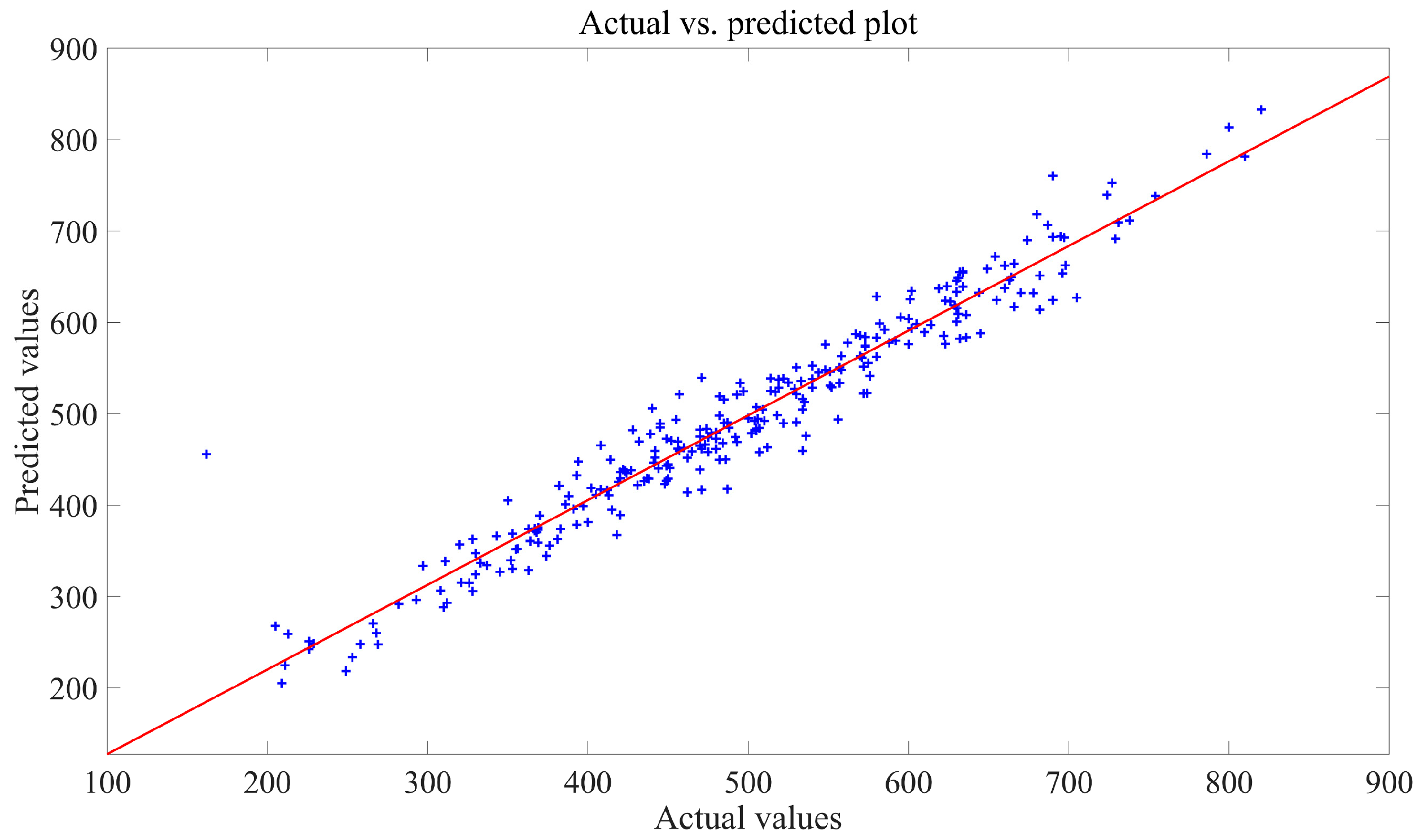
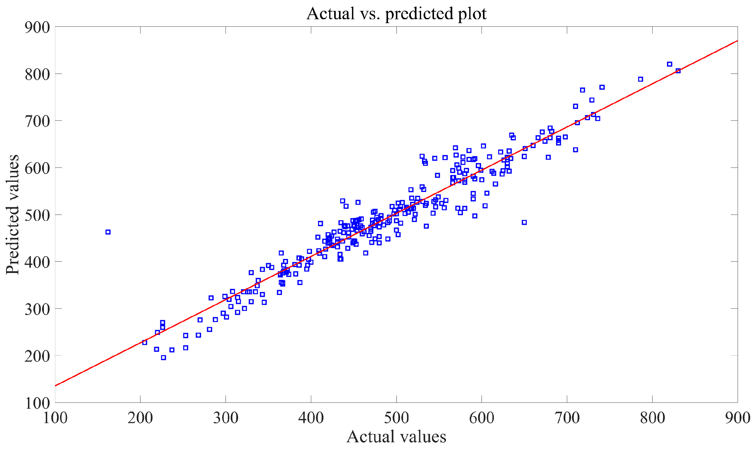
To assess the effectiveness of prediction models, regression plots were used. In these plots (refer to
Figure 5,
Figure 6,
Figure 7 and
Figure 8), the horizontal axis represents the true data values, while the vertical axis displays the predicted values. Each sample point on the plot is positioned based on both the actual and predicted values. When the predicted values match the actual values, all sample points align perfectly along a straight line that follows the diagonal of the plot. The Ordinary Least Squares Regression (OLS) method is applied to determine the least-square line for these sample points. The closer this line aligns with the diagonal, the higher the accuracy of the forecast.
The figures indicate that the majority of sample points in the regression plot for the SMA-SVR model are clustered closely around the least-square line, suggesting a high level of prediction accuracy and robustness across various test sets. On the contrary, sample points from the other three models exhibit notable deviations from their respective least-square lines, suggesting a higher likelihood of significant prediction errors in multiple predictions made using GWO-SVR, PSO-BP, and SSA-Elman.
The results of the multiple comparison tests are tabulated in
Table 4, with the best hybrid model labeled as “1”, followed by the second-best as “2”, and so forth. It is noteworthy that, among all the models under comparison, SMA-SVR emerges as the top performer in predictive capabilities.
3.3. Tests and Discussion of 0.2% Proof Stress Prediction
In materials exhibiting non-linear behavior or inelasticity, such as low-alloy steel, determining the yield point often necessitates the use of the 0.2% offset method. Within the realm of engineering, the 0.2% proof stress serves as a crucial indicator for the yield stress of steel. Like other elastic materials, steel elongates and deforms when subjected to stress. Upon stress release, the material is expected to revert to its original dimensions. However, if the stress surpasses a critical value, the material endures permanent deformation, marking the onset of a plastic zone or the attainment of the yield point. Accordingly, the proof stress signifies the elastic limit of the material, which is a pivotal parameter in engineering design. Typically, this value is derived by drawing a line parallel to the stress–strain curve at the 0.2% strain value.
To assess the efficacy of hybrid models in predicting the 0.2% proof stress of low-alloy steel, this section focused on the elemental composition and operating temperatures as input variables. The target prediction variable remained at 0.2% proof stress. A random selection of 640 sample entries from the dataset constituted the training set, while the remaining 274 samples were allocated to the test set, maintaining a consistent training-to-test ratio of 7:3. The procedural aspects of training and testing for the four hybrid models mirrored those of the prior evaluation, with hardware specifications, population size, and iteration counts remaining consistent. The outcomes of the 0.2% proof stress prediction tests are detailed in
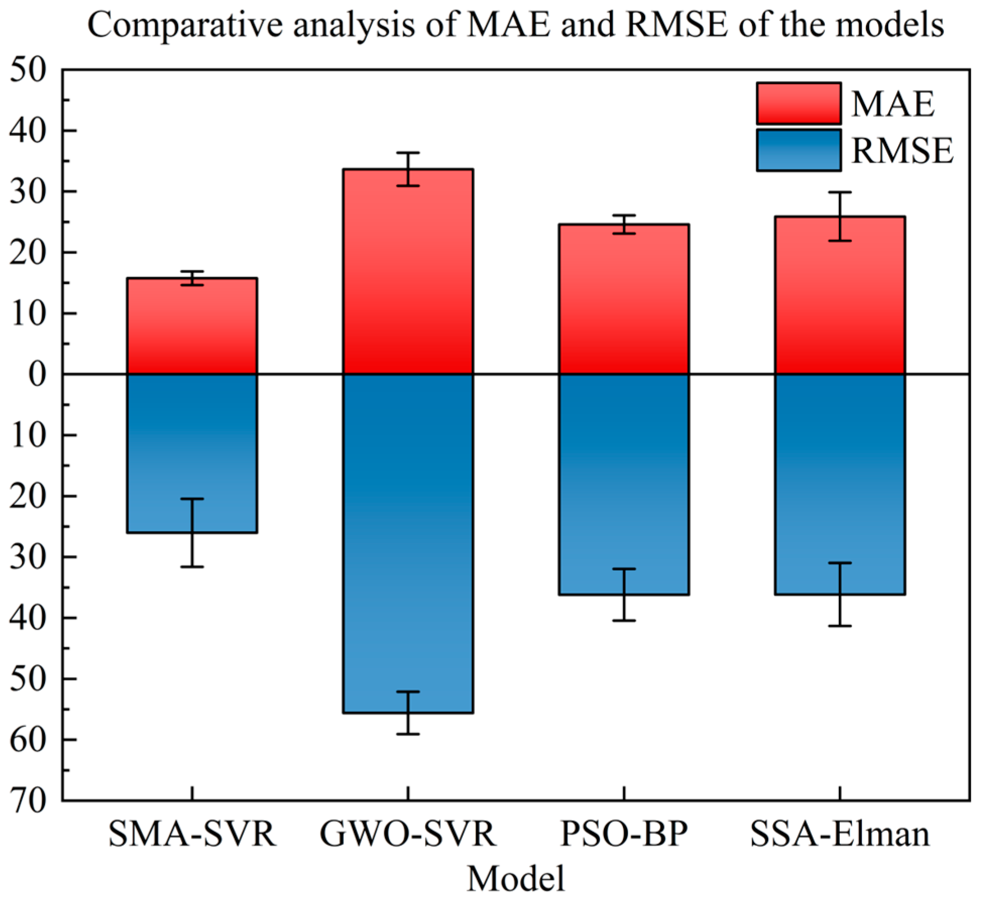
Table 5 for reference. A bar chart with the MAE and RMSE data of the experimental results is further plotted for a visual comparison of the prediction performance of these models, as shown in
Figure 9.
The analysis of predicting 0.2% proof stress by the models indicates that SMA-SVR achieves the highest prediction accuracy among them, with an R2 ranking of SMA-SVR > PSO-BP > SSA-Elman > GWO-SVR. Furthermore, SMA-SVR demonstrates the lowest values for MAE and RMSE. In addition, SMA-SVR has the shortest computational time for both training and testing, representing only 32.50% of GWO-SVR and 18.99% of SSA-Elman.
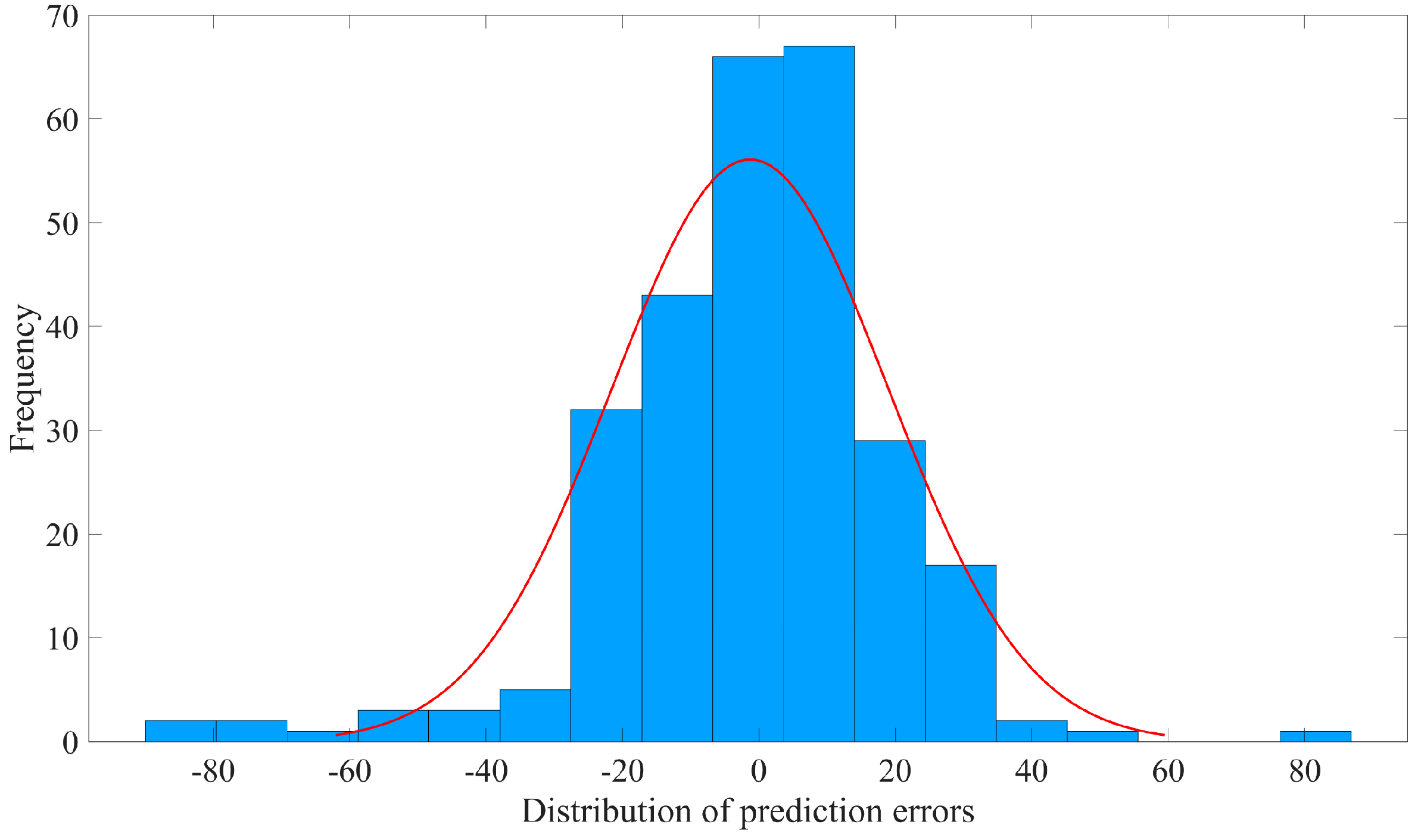
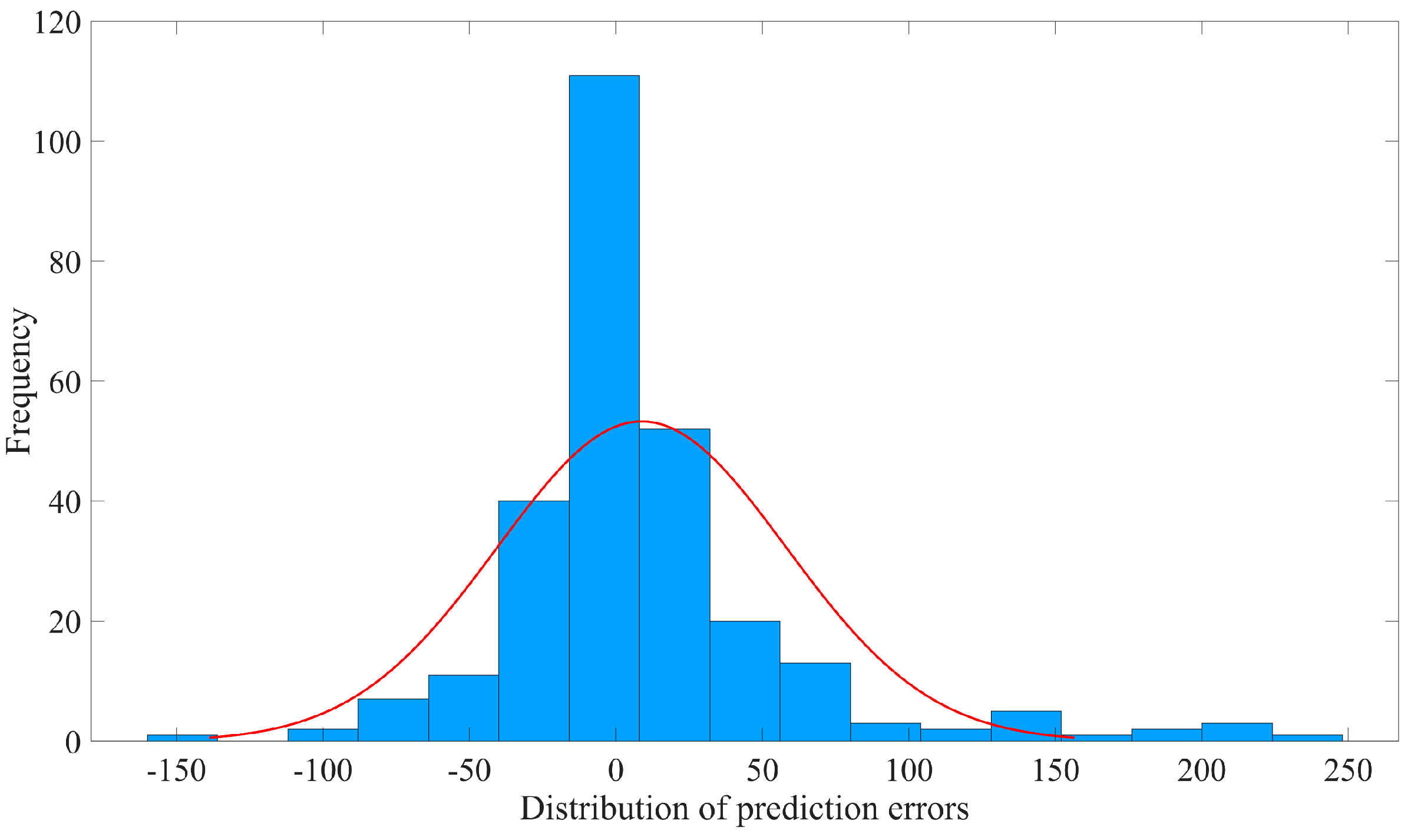
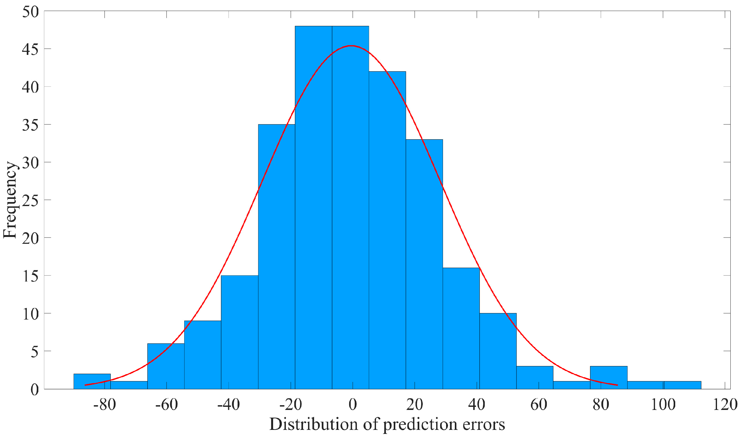
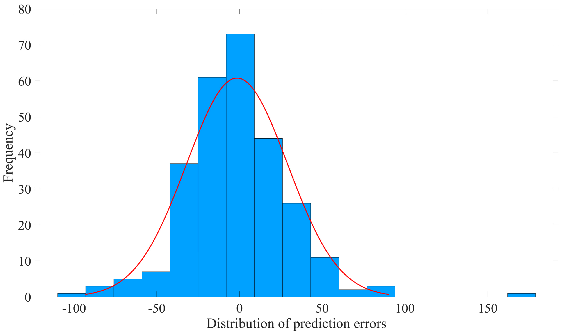
An analysis of the prediction errors of each model was also conducted separately. Initially, a normality test was performed using the Shapiro–Wilk test method, considering the small sample sizes in each group. The results of the normality test can be found in
Table 6.
The normality test conducted on the prediction errors indicates that the models do not follow a normal distribution at a significance level of 1% (all
p-values are below 0.05). Consequently, a detailed analysis of the error distributions was conducted, and error histograms for each model were created, as illustrated in
Figure 10,
Figure 11,
Figure 12 and
Figure 13.
The prediction errors of SMA-SVR are primarily clustered in the range of [−25, 25], with absolute error values generally below 90. In contrast, the prediction errors of GWO-SVR are predominantly found within the range of [−30, 30], but a considerable number of samples exhibit an absolute error exceeding 90, with four samples exhibiting values exceeding 200. While the errors tend to be centered around 0, the deviations from the actual values significantly diminish the reliability of GWO-SVR predictions.
The prediction errors of PSO-BP are mainly distributed within the interval of [−40, 40], with some samples falling in the ranges of [−70, −40] and [40, 70] and two samples showing absolute errors exceeding 90. Similarly, the prediction errors of SSA-Elman are concentrated in the range of [−45, 45], with only two samples exhibiting an absolute error exceeding 90 and one sample showing a prediction error of more than 160 for the absolute value.
Overall, the prediction performance of SMA-SVR surpasses all the other models, with error values predominantly centered around 0 and absolute errors mostly below 90. As a result, SMA-SVR stands out as the most reliable model among the models considered.
4. Prediction Tests with Data from the Universal Testing Machine
Tensile tests were carried out on 30 varieties of low-alloy steel, utilizing a universal testing machine (UTM). The resulting data on tensile strength and 0.2% proof stress were collected. Subsequently, a comparative analysis and discussion were conducted to further evaluate the predictive capabilities of the hybrid models.
4.1. Material Preparation and Experiment Design
In total, 30 types of low-alloy steel were selected based on their mechanical properties and intended usage scenarios. Detailed information about these steel types can be found in
Table 7, where they are categorized into nine distinct groups, including corrosion-resistant steel, high-strength steel, structural steel, and welded weathering steel.
Table 8 records the elemental compositions of these low-alloy steel types.
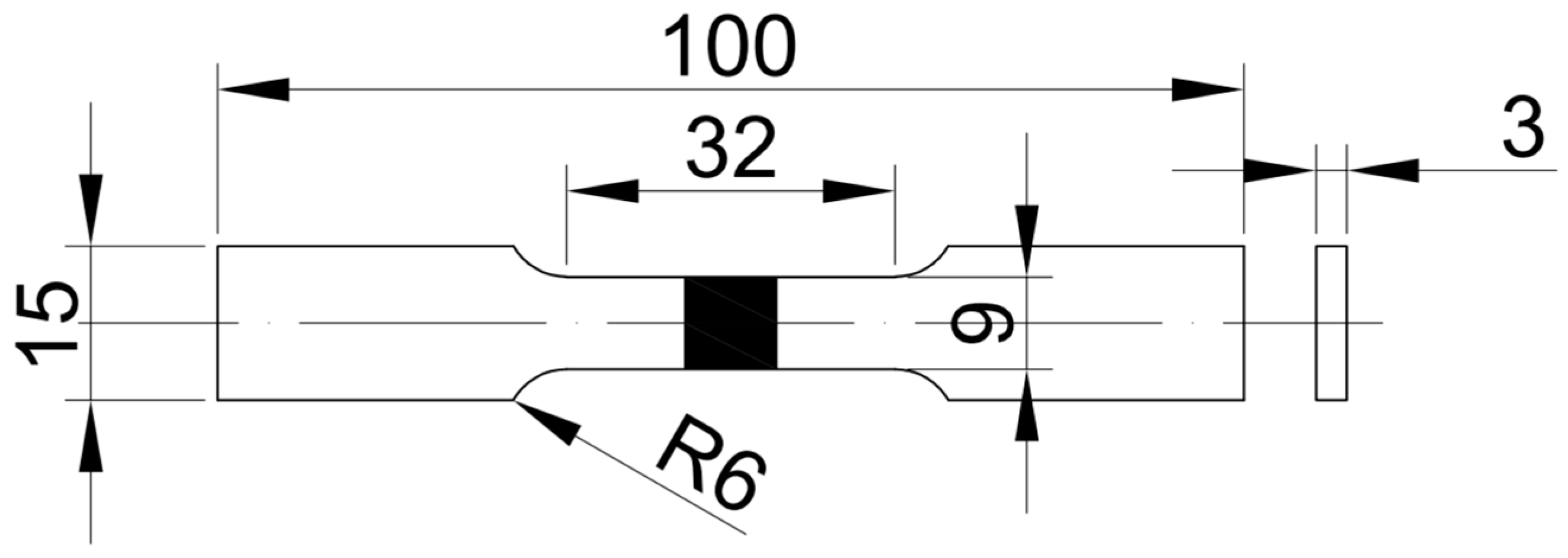
To create the test samples, 1500 mm × 1000 mm × 5 mm steel plates were utilized for each steel type. These plates underwent wire cutting and grinding processes following the design drawing of the test piece (refer to
Figure 14). For every grade of steel, three test pieces were meticulously prepared, and each test piece underwent three separate tensile tests. The average values of tensile strength and 0.2% proof stress derived from these tests were collected as test data.
The material preparation procedure was carefully crafted to ensure uniformity and consistency among the specimens. Through the wire-cutting and grinding processes, the specimens were standardized in dimensions and surface finish, thereby reducing any potential impact on the experimental outcomes. Conducting three tests for each test piece enabled us to acquire dependable and consistent data for all types of steel.
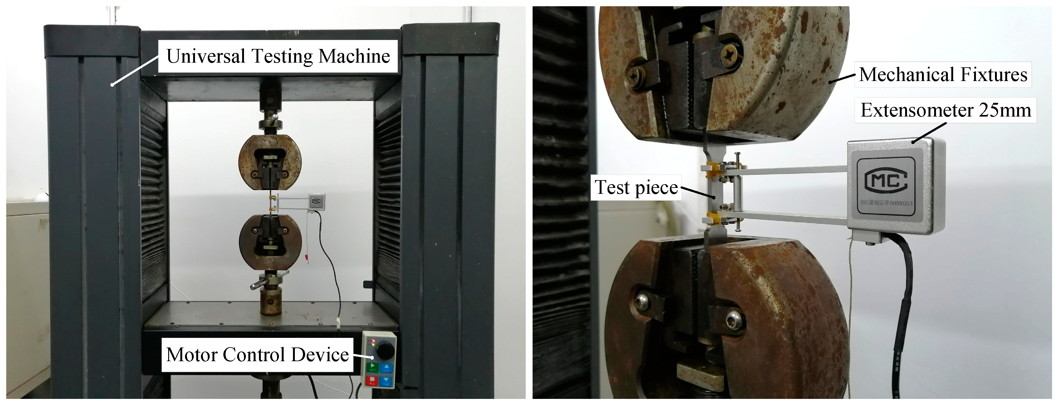
The universal testing machine (UTM) used was HDW-50k with the following parameters: maximum range: 5 × 10⁵ N; accuracy level: 1st rank; error of the indicated value: ±1.0%; load measurement range: 2~100% of the full range; and displacement resolution: 1 × 10⁻² mm. The extensometer’s scale distance for tests is 25 mm, with a relative error of ±1.0% for both the scale distance and the indicated value.
The experimental process involves using the UTM sensor to measure the force on the test pieces and the extensometer to determine their deformation. Photographs of the test site can be found in
Figure 15. The specific steps are as follows:
- (1)
Mount the test piece in the UTM collet with the extensometer fixed in the middle.
- (2)
Axially stretch the test piece using the UTM with a strain rate set to 1.0 mm/min.
- (3)
Measure the force of the test piece with the UTM force sensor and the deformation with the extensometer.
- (4)
During the test, real-time measurement information is output to UTM software (UTM, Orlando, FL, USA,
https://getutm.app) for processing.
- (5)
After the test, software is used to calculate the measured information, obtaining the data for tensile strength and 0.2% proof stress.
4.2. Evaluation and Performance Analysis
The predictive capabilities of the four hybrid models are assessed by estimating the tensile strength and 0.2% proof stress of low-alloy steel based on their elemental composition as the input features. The dataset comprises 30 entries, with 21 entries randomly allocated to the training set and the remaining 9 to the test set, maintaining a 7:3 ratio between the training and test sets. Throughout the experiments, the hardware configuration of the computer remained constant, while specific parameters were adjusted as detailed below. For both SMA-SVR and GWO-SVR, the population size was fixed at 200, and the maximum number of iterations was set to 300. The penalty factor ranged between 0.01 and 800, and the kernel parameter was between 0.001 and 50. In the case of PSO-BP, the particle size was set to 30, and the maximum number of iterations was capped at 100, while the hidden layer of the BP network housed 7 nodes. As for SSA-Elman, the sparrow population size was 50, and the maximum number of iterations for the Elman network was set at 1000.
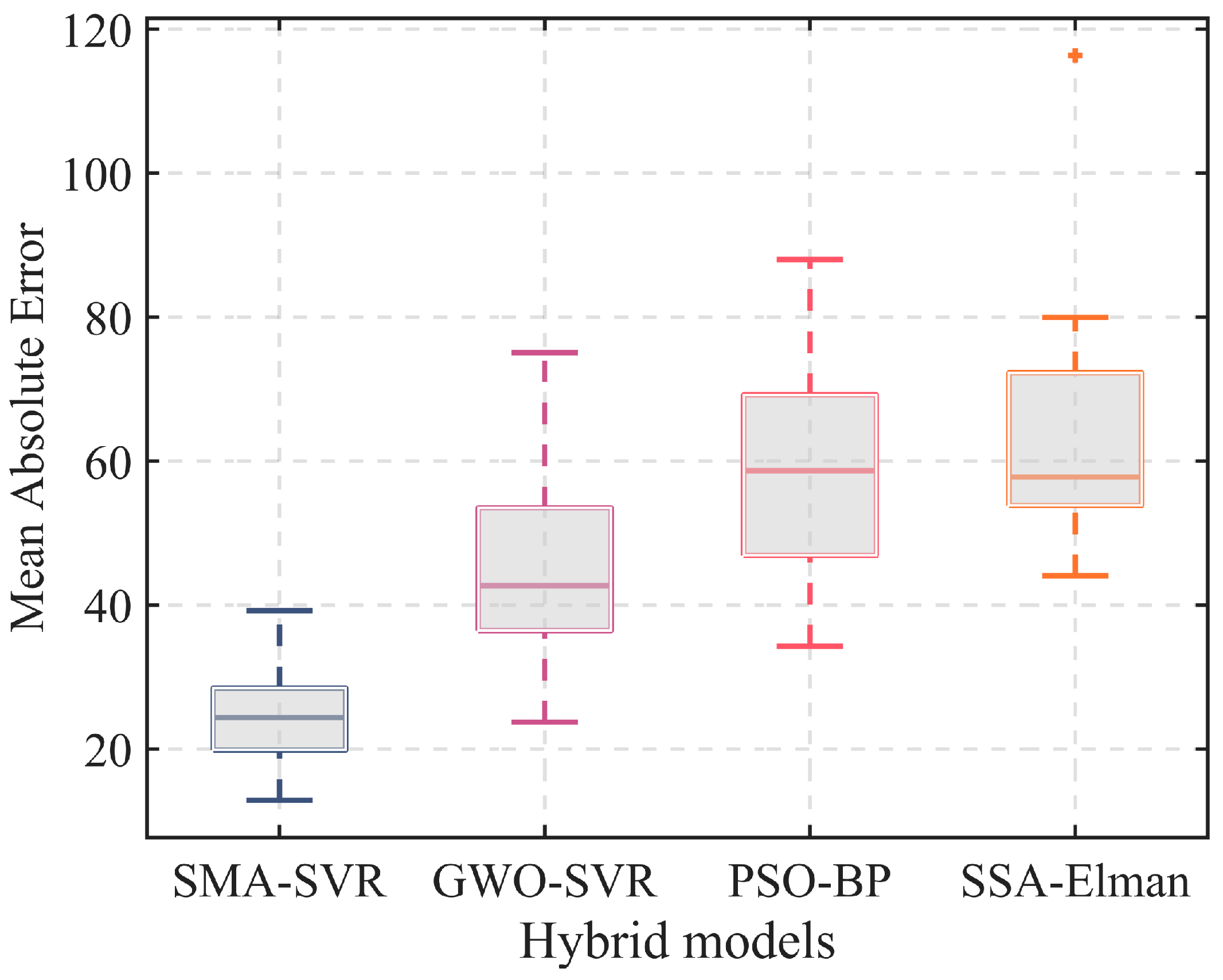
Each model underwent 20 repetitions to acquire prediction results and evaluation metrics, as summarized in
Table 9. To illustrate prediction errors visually, box plots depicting MAE were generated, as depicted in
Figure 16. Regarding the prediction of tensile strength, SSA-Elman emerged as the hybrid model with the least favorable performance. Despite its commendable accuracy, it was burdened with prolonged computational time and yielded higher MAE and MSE values when contrasted with the other models. In comparison, while PSO-BP exhibited a lower prediction error than SSA-Elman, its R
2 value was the most modest, signifying challenges in comprehending the intricate mapping relationship between the material composition and properties.
SMA-SVR and GWO-SVR, both known for their suitability in small sample sizes, outperformed the previous two models. SMA-SVR demonstrates the highest R2 value, which is approximately twice as high as that of GWO-SVR. Moreover, SMA-SVR exhibits a 44.92% smaller MAE value than GWO-SVR, with a shorter computational time. In the 20 conducted tests, SMA-SVR yielded the most favorable outcomes with a penalty factor set to 450.5898 and a kernel parameter set to 0.0073. The resulting values for MAE, MSE, R2, and computational times were 12.5516, 296.5571, 0.9593, and 9.1410 s, respectively. Conversely, GWO-SVR delivered optimal results when the penalty factor was set to 800.0 and the kernel parameter to 0.7702. Under these settings, GWO-SVR displays an MAE of 20.0123, an MSE of 618.0679, an R2 of 0.9324, and a computational time of 10.9094 s.
According to the findings, SMA-SVR exhibits the most robust modeling capability among the four hybrid models. Its predictions are not only accurate but also efficient, rendering it a prudent choice for predicting the tensile strength of low-alloy steel.
The test results and error measurements of 0.2% proof stress prediction are recorded in
Table 10. Based on the experimental results of 0.2% proof stress, a dual
Y-axis graph combining a bar chart and a line graph is plotted to visually demonstrate the prediction performance of each model, as shown in
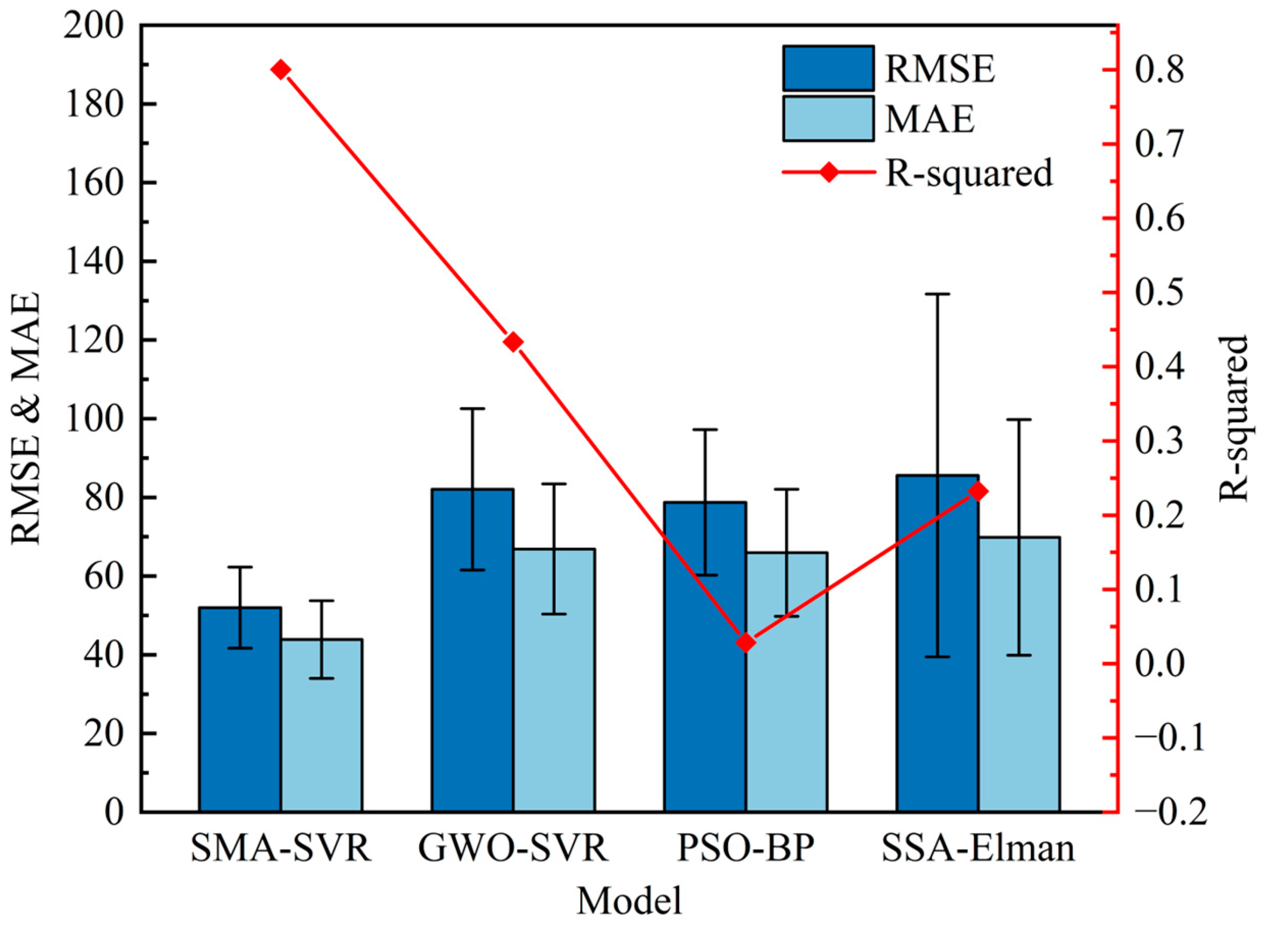
Figure 17. It includes the RMSE, MAE, and R-squared data. SMA-SVR also stands out as the best model with the smallest MAE and MSE values, as well as the shortest computational time. This test further demonstrates its robustness. However, a closer examination of the best prediction results from each model reveals some intriguing phenomena.
With the penalty factor set to 536.0331 and the kernel parameter set to 0.0214, SMA-SVR produced the most accurate predictions, achieving an R2 value of 0.9117, RMSE of 30.1331, and MAE of 24.9031. Interestingly, the second-best performing model was not GWO-SVR but rather SSA-Elman, which yielded an R2 value of 0.8434, RMSE of 49.2817, and MAE of 42.2157. This outcome underscores the critical impact of hyperparameter optimization on the learning capabilities of models. The selection of appropriate hyperparameters leads to a considerable improvement in both computational time and prediction accuracy.
The combination of SMA and SVR proves to be highly successful, with the hyperparameter optimization of SMA significantly outperforming that of GWO. The prediction performance and computational efficiency of SMA-SVR are optimal among the experiments conducted. SMA-SVR demonstrates an exceptional ability to learn the complex mapping between chemical compositions and material properties, even with small sample sizes. Moreover, it exhibits a strong generalization ability. These findings support the argument that SMA-SVR is an ideal choice for predicting the 0.2% proof stress of low-alloy steel.


