Analytical Study of Nonlinear Systems of Higher-Order Difference Equations: Solutions, Stability, and Numerical Simulations

Abstract

This paper aims to derive analytical expressions for solutions of fractional bidimensional systems of difference equations with higher-order terms under specific parametric conditions. Additionally, formulations of solutions for one-dimensional equations derived from these systems are explored. Furthermore, rigorous proof is provided for the local stability of the unique positive equilibrium point of the proposed systems. The theoretical findings are validated through numerical examples using MATLAB, facilitating graphical illustrations of the results.

1. Introduction

Difference equations and systems constitute a foundational element of mathematical modeling, exerting significant influence across a spectrum of scientific domains and practical applications. Over the past decade, this field has witnessed a notable evolution, characterized by a surge in scholarly interest and activity. This trend underscores an increasingly recognized importance and utility of difference equations and systems in tackling intricate phenomena and facilitating informed decision-making processes.

In recent years, there has been a growing emphasis on exploring nonlinear systems of difference equations, driven by a quest for analytical solutions, deeper insights into dynamic behaviors, and applications spanning diverse disciplines including biology, physics, probability theory, environmental science, and engineering. These systems serve as discrete analogs to differential equations, offering a robust framework for modeling time-series data such as economic indicators (e.g., Gross Domestic Product, inflation rates, exchange rates) inherently measured at discrete intervals (see, [1,2]). Existing research has probed various facets of nonlinear dynamics, encompassing local dynamics, topological classifications, bifurcation analysis, and chaos control. For example, Khan et al. [3] investigated these dynamics within the context of a discrete-time COVID-19 epidemic model, while other studies [4,5] have explored similar phenomena across different domains. However, while several methods exist for solving linear difference equations, the landscape of nonlinear systems remains largely uncharted. Despite recent attempts to simplify complex nonlinear systems into linear forms, there persists a significant gap in analytical approaches for addressing systems of difference equations, posing a challenge for researchers striving to deepen their understanding of their behavior and properties (see, [6,7]).

The heightened interest in nonlinear systems of difference equations underscores their potential to capture intricate dynamics and phenomena that may elude representation by linear models. Nonlinear systems often exhibit rich behavior, including bifurcations, chaos, and complex attractors, rendering them valuable tools for comprehending the dynamics of real-world phenomena. A particularly active area of research centers on the pursuit of closed-form solutions to nonlinear systems of difference equations, to enhance our understanding of dynamic systems and refine predictions with greater precision. (see, [8,9,10,11,12,13]). Many researchers have made significant contributions to unraveling the behavior of solved difference equations and systems, shedding light on their dynamics and stability properties. For instance, Elsayed and Alshabi [14] delved into the solution forms and stability properties of second-order systems, while Al-Basyouni and Elsayed [15] provided formulas for solutions to systems of rational difference equations of various orders, demonstrating periodicity in certain cases. Okumuş and Soykan [16] extended this exploration to two-dimensional systems associated with Tribonacci numbers. Our paper extends beyond these realms by delving into the analysis of higher-order systems and considering more diverse and complex scenarios. By addressing specific systems of difference equations and investigating their existence, form, and stability properties, our paper offers a comprehensive examination of nonlinear dynamics in discrete time. Furthermore, we can obtain numbers that satisfy some conditions of interest, for example, Richard and Raoul numbers. Moreover, our paper builds upon the contributions of Ghezal and Zemmouri [12] and Abo-Zeid et al. [6,7] by synthesizing and advancing existing knowledge in the field of nonlinear difference equations and systems. By incorporating recent advancements in theoretical analysis and numerical validation techniques, our study pushes the boundaries of understanding in this domain and opens up new avenues for exploration. While Abo-Zeid [17] provides explicit solutions for specific difference equations, our paper explores the fundamental properties of systems of difference equations representing different analytical challenges. Our work provides a deeper analysis of the behavior of bidimensional systems, while Abo-Zeid’s [17] work revolves around studying the details of explicit solutions and the general behavior of specific models. The study by Simşek et al. [18] focuses on solving a specific rational difference equation, with a particular focus on providing explicit solutions and analyzing the behavior of the solutions. In contrast, our paper delves into the examination of a broader range of rational difference equations, exploring various forms and complexities.

In comparing our paper to existing research, we identify opportunities to build upon current knowledge and extend the frontier of understanding in this field. Through rigorous theoretical analysis and numerical validation, our paper aims to fill critical gaps in the literature by addressing specific systems of difference equations and investigating their existence, form, and stability properties. By elucidating the dynamics of nonlinear systems in discrete time, our work seeks to advance the understanding of complex mathematical models and their applications across various scientific and engineering domains. Specifically, in this paper, we focus on exploring the existence and form of solutions for the systems of Difference Equations (1)–(4).

The remainder of this paper is structured as follows: Section 1 offers a detailed review of the literature, highlighting key developments and identifying gaps that motivate the current study. In Section 2, we present the theoretical framework and methodologies employed in our analysis, laying the groundwork for subsequent discussions. Section 3 delves into the empirical findings, presenting numerical simulations and graphical illustrations that corroborate the theoretical insights. Finally, Section 4 synthesizes the key findings, discusses their implications, and outlines avenues for future research.

2. Main Results

In this paper, we delve into the examination of the subsequent systems of rational difference equations:

$$\begin{array}{cc}\hfill \forall n\ge 0,{\sigma }_{n+1}={\displaystyle \frac{1}{1+{\rho }_n\left(1-{\sigma }_{n-1}{\rho }_{n-2}\right)}},& {\rho }_{n+1}={\displaystyle \frac{1}{1+{\sigma }_n\left(1-{\rho }_{n-1}{\sigma }_{n-2}\right)}},\end{array}$$

(1)

endowed with initial conditions denoted as ${\sigma }_{-2}$, ${\sigma }_{-1}$, ${\sigma }_0$, ${\rho }_{-2}$, ${\rho }_{-1}$, and ${\rho }_0$, ensuring that they are real and non-zero.

$$\begin{array}{cc}\hfill \forall n& \ge 0,{\sigma }_{n+1}={\displaystyle \frac{1}{1+{\rho }_{n-q}\left(1-{\sigma }_{n-2q-1}{\rho }_{n-3q-2}\right)}},\hfill \\ \hfill {\rho }_{n+1}& ={\displaystyle \frac{1}{1+{\sigma }_{n-q}\left(1-{\rho }_{n-2q-1}{\sigma }_{n-3q-2}\right)}},q\ge 0,\hfill \end{array}$$

(2)

endowed with initial conditions denoted as ${\sigma }_{-j}$, and ${\rho }_{-j}$, $j\in \left\{0,1,\dots ,3q+2\right\}$, ensuring that they are real and non-zero.

$$\begin{array}{cc}\hfill \forall n& \ge 0,{\sigma }_{n+1}={\displaystyle \frac{1}{-1+{\rho }_n\left(1+{\sigma }_{n-1}\left(2+{\rho }_{n-2}\right)\right)}},\hfill \\ \hfill {\rho }_{n+1}& ={\displaystyle \frac{1}{-1+{\sigma }_n\left(1+{\rho }_{n-1}\left(2+{\sigma }_{n-2}\right)\right)}},\hfill \end{array}$$

(3)

endowed with initial conditions denoted as ${\sigma }_{-2}$, ${\sigma }_{-1}$, ${\sigma }_0$, ${\rho }_{-2}$, ${\rho }_{-1}$, and ${\rho }_0$, ensuring that they are real and non-zero.

$$\forall n\ge 0,{\sigma }_{n+1}={\displaystyle \frac{1}{-1+{\rho }_{n-q}\left(1+{\sigma }_{n-2q-1}\left(2+{\rho }_{n-3q-2}\right)\right)}},$$

(4)

$${\rho }_{n+1}={\displaystyle \frac{1}{-1+{\sigma }_{n-q}\left(1+{\rho }_{n-2q-1}\left(2+{\sigma }_{n-3q-2}\right)\right)}},q\ge 0,$$

endowed with initial conditions denoted as ${\sigma }_{-j}$, and ${\rho }_{-j}$, $j\in \left\{0,1,\dots ,3q+2\right\}$, ensuring that they are real and non-zero. To ensure the robustness and validity of the systems under consideration, the denominators must remain non-zero to prevent any division by zero errors. Hence, a critical condition governing these denominators is that the expression within them should never equate to zero for all $n\ge 0$. By imposing this condition, we guarantee the stability and solvability of the system, thereby facilitating a comprehensive and accurate analysis of its behavior and properties. The physical background of the systems of rational difference equations described in Equations (1)–(4) lies in their representation of dynamic processes influenced by feedback mechanisms. These systems model scenarios where quantities or variables interact with each other over discrete time intervals, and their behavior depends on their past values and certain parameters. System (1) represents a feedback loop where two variables, $\sigma$ and $\rho$, influence each other’s evolution over time. The evolution of each variable depends on its past values and the other variable’s value at the previous time step. This system could describe phenomena in various fields such as population dynamics, economic systems, or chemical reactions in which two entities interact in a feedback loop. System (2) extends the concept of (1) by introducing a delay parameter q, indicating that the influence between $\sigma$ and $\rho$ occurs over multiple time steps. This delay could represent phenomena in which there is a time lag between the cause and effect in the system, such as in delayed feedback control systems or systems with transport delays. System (3) introduces nonlinearities in the feedback loop by incorporating quadratic terms in the evolution equations of $\sigma$ and $\rho$. This nonlinearity can capture more complex dynamics compared to linear feedback systems. It may be relevant in systems in which interactions between variables exhibit nonlinear behavior, such as in biological systems or nonlinear control systems. System (4) extends the nonlinear feedback model of (3) by introducing a delay parameter q, similar to (2). This combination of nonlinearities and delay further enriches the dynamics of the system, allowing for the modeling of more intricate feedback mechanisms with time delays. These systems of rational difference equations provide mathematical frameworks for understanding the behavior of dynamic systems subject to feedback interactions and time delays, with applications ranging from natural and social sciences to engineering and control theory.

In the context of this study, we thoroughly examine the well-defined solutions of the previously mentioned systems, elucidating their forms and behaviors. This analytical scrutiny is carried out through the introduction of specific substitutions to the phase variables:

$$\begin{array}{cc}\hfill \forall n,{\sigma }_n={\displaystyle \frac{{\pi }_{n-1}}{{\omega }_n}},& {\rho }_n={\displaystyle \frac{{\omega }_{n-1}}{{\pi }_n}}.\end{array}$$

(5)

Remark 1. 

The term ’well-defined solutions’ for Systems (1)–(4) refers to solutions derived from the sets $\mathcal{F}=\left\{{\sigma }_{-2},{\sigma }_{-1},{\sigma }_0,{\rho }_{-2},{\rho }_{-1},\mathit{and}{\rho }_0\right\}$, selected outside the respective singularity sets of the systems. A set of $\mathcal{F}$ that produces a solution $\left\{\left({\sigma }_n,{\rho }_n\right),n\ge 1\right\}$ for (1), wherein at least one denominator becomes zero at some least index n, leads to an undefined value for ${\sigma }_{n+1}$ and/or ${\rho }_{n+1}$. This particular set is commonly referred to as the ’forbidden set,’ as discussed further in [19].

2.1. Formulation of Solutions for System (1)

To derive the closed-form solutions for the system represented by (1), we employ the substitution defined in (5). Following some transformations, we arrive at the subsequent system of linear difference equations:

$$\begin{gathered} \begin{array}{cc}\hfill \forall n\ge 0,{\displaystyle \frac{{\omega }_{n+1}}{{\pi }_n}}=1+{\displaystyle \frac{{\omega }_{n-1}}{{\pi }_n}}\left(1-{\displaystyle \frac{{\pi }_{n-2}}{{\omega }_{n-1}}}{\displaystyle \frac{{\omega }_{n-3}}{{\pi }_{n-2}}}\right),& {\displaystyle \frac{{\pi }_{n+1}}{{\omega }_n}}=1+{\displaystyle \frac{{\pi }_{n-1}}{{\omega }_n}}\left(1-{\displaystyle \frac{{\omega }_{n-2}}{{\pi }_{n-1}}}{\displaystyle \frac{{\pi }_{n-3}}{{\omega }_{n-2}}}\right),\end{array} \\ \Updownarrow \end{gathered}$$

$$\begin{array}{cc}\hfill \forall n\ge 0,{\omega }_{n+1}={\pi }_n+{\omega }_{n-1}-{\omega }_{n-3},& {\pi }_{n+1}={\omega }_n+{\pi }_{n-1}-{\pi }_{n-3}.\end{array}$$

(6)

By manipulating System (6), we derive the subsequent system

$$\forall n\ge 0,\left\{\begin{array}{c}{\omega }_{n+1}+{\pi }_{n+1}=\left({\omega }_n+{\pi }_n\right)+\left({\omega }_{n-1}+{\pi }_{n-1}\right)-\left({\omega }_{n-3}+{\pi }_{n-3}\right)\hfill \\ {\omega }_{n+1}-{\pi }_{n+1}=-\left({\omega }_n-{\pi }_n\right)+\left({\omega }_{n-1}-{\pi }_{n-1}\right)-\left({\omega }_{n-3}-{\pi }_{n-3}\right)\hfill \end{array},\right.$$

(7)

which transforms into a system of two independent linear difference equations

$$\begin{array}{cc}\hfill \forall n\ge 0,{\epsilon }_{n+1}={\epsilon }_n+{\epsilon }_{n-1}-{\epsilon }_{n-3},& {\tau }_{n+1}=-{\tau }_n+{\tau }_{n-1}-{\tau }_{n-3}.\end{array}$$

(8)

This transformation is achieved through the following change of variables: $\forall n,$ ${\epsilon }_n={\omega }_n+{\pi }_n$ and ${\tau }_n={\omega }_n-{\pi }_n$. Therefore, the exact closed-form of the general solution for System (8) (resp. System (6)) is derived, as detailed in the following Lemma 1 (resp. Lemma 2).

Lemma 1. 

Let $\left\{\left({\epsilon }_n,{\tau }_n\right),n\ge -3\right\}$ be the solution to System (8), which comprises homogeneous linear difference equations with constant coefficients along with initial conditions ${\epsilon }_{-3}$, ${\epsilon }_{-2}$, ${\epsilon }_{-1}$, ${\epsilon }_0$, ${\tau }_{-3}$, ${\tau }_{-2}$, ${\tau }_{-1}$, and ${\tau }_0\in \mathbb{R}$. For all $n\ge 0,$ the solutions are given by

$$\begin{array}{cc}\hfill \forall n,{\epsilon }_n& ={\alpha }_1^n{f}_1\left({\epsilon }_{-3},{\epsilon }_{-2},{\epsilon }_{-1},{\epsilon }_0\right)+{\alpha }_2^n{f}_2\left({\epsilon }_{-3},{\epsilon }_{-2},{\epsilon }_{-1},{\epsilon }_0\right)\hfill \\ \hfill & +{\alpha }_3^n{f}_3\left({\epsilon }_{-3},{\epsilon }_{-2},{\epsilon }_{-1},{\epsilon }_0\right)+f_4\left({\epsilon }_{-3},{\epsilon }_{-2},{\epsilon }_{-1},{\epsilon }_0\right),\hfill \end{array}$$

$$\begin{array}{cc}\hfill \forall n,{\left(-1\right)}^n{\tau }_n& ={\alpha }_1^n{g}_1\left({\tau }_{-3},{\tau }_{-2},{\tau }_{-1},{\tau }_0\right)+{\alpha }_2^n{g}_2\left({\tau }_{-3},{\tau }_{-2},{\tau }_{-1},{\tau }_0\right)\hfill \\ \hfill & +{\alpha }_3^n{g}_3\left({\tau }_{-3},{\tau }_{-2},{\tau }_{-1},{\tau }_0\right)+g_4\left({\tau }_{-3},{\tau }_{-2},{\tau }_{-1},{\tau }_0\right).\hfill \end{array}$$

Proof. 

In solving the first (respectively, second) linear difference equation of System (8), we typically utilize the characteristic polynomial:

$${\lambda }^4-{\lambda }^3-{\lambda }^2+1=\left(\lambda -1\right)\left(\lambda -{\tilde{\alpha }}_1\right)\left(\lambda -{\tilde{\alpha }}_2\right)\left(\lambda -{\tilde{\alpha }}_3\right)=0,$$

(respectively,

$${\lambda }^4+{\lambda }^3-{\lambda }^2+1=\left(\lambda +1\right)\left(\lambda +{\tilde{\alpha }}_1\right)\left(\lambda +{\tilde{\alpha }}_2\right)\left(\lambda +{\tilde{\alpha }}_3\right)=0).$$

The roots of this equation are

$${\lambda }_1=1,{\lambda }_2={\tilde{\alpha }}_1,{\lambda }_3={\tilde{\alpha }}_2,{\lambda }_4={\tilde{\alpha }}_3,$$

(respectively,

$${\lambda }_1=-1,{\lambda }_2=-{\tilde{\alpha }}_1,{\lambda }_3=-{\tilde{\alpha }}_2,{\lambda }_4=-{\tilde{\alpha }}_3),$$

where ${\tilde{\alpha }}_1$ and ${\tilde{\alpha }}_2$ are a pair of complex conjugate roots, and ${\tilde{\alpha }}_3$ is a real root satisfying the following conditions:

$$\begin{array}{ccc}\hfill 1-{\displaystyle \prod _{t=1}^3}{\tilde{\alpha }}_t=0,& {\displaystyle \sum _{t=1}^3}{\tilde{\alpha }}_t=0,& 1+{\displaystyle \prod _{1\le t_1<t_2\le 3}}{\tilde{\alpha }}_{t_1}{\tilde{\alpha }}_{t_2}=0.\hfill \end{array}$$

(9)

Hence, the closed form of the general solution for the first (respectively, second) linear difference equation of system (8) is given by:

$$\forall n\ge -3,{\epsilon }_n={\beta }_1{\alpha }_1^n+{\beta }_2{\alpha }_2^n+{\beta }_3{\alpha }_3^n+{\beta }_4,$$

where ${\alpha }_1,$ ${\alpha }_2$ and ${\alpha }_3$ are real roots satisfying: $2{\alpha }_1={\tilde{\alpha }}_1+{\tilde{\alpha }}_2,$ $2i{\alpha }_2={\tilde{\alpha }}_1-{\tilde{\alpha }}_2,$ ${\alpha }_3={\tilde{\alpha }}_3$ and i is a complex number satisfying: $i^2=-1$ (respectively,

$$\forall n\ge -3,{\tau }_n={\left(-1\right)}^n\left({\overline{\beta }}_1{\alpha }_1^n+{\overline{\beta }}_2{\alpha }_2^n+{\overline{\beta }}_3{\alpha }_3^n+{\overline{\beta }}_4\right)).$$

Here, ${\epsilon }_{-3}$, ${\epsilon }_{-2}$, ${\epsilon }_{-1}$, ${\epsilon }_0$, ${\tau }_{-3}$, ${\tau }_{-2}$, ${\tau }_{-1}$, and ${\tau }_0$ are initial conditions such that:

$$\left\{\begin{array}{c}{\epsilon }_0={\beta }_1+{\beta }_2+{\beta }_3+{\beta }_4\hfill \\ {\epsilon }_{-1}={\displaystyle \genfrac{}{}{1.0pt}{}{{\beta }_1}{{\alpha }_1}}+{\displaystyle \frac{{\beta }_2}{{\alpha }_2}}+{\displaystyle \frac{{\beta }_3}{{\alpha }_3}}+{\beta }_4\hfill \\ {\epsilon }_{-2}={\displaystyle \genfrac{}{}{1.0pt}{}{{\beta }_1}{{\alpha }_1^2}}+{\displaystyle \frac{{\beta }_2}{{\alpha }_2^2}}+{\displaystyle \frac{{\beta }_3}{{\alpha }_3^2}}+{\beta }_4\hfill \\ {\epsilon }_{-3}={\displaystyle \genfrac{}{}{1.0pt}{}{{\beta }_1}{{\alpha }_1^3}}+{\displaystyle \frac{{\beta }_2}{{\alpha }_2^3}}+{\displaystyle \frac{{\beta }_3}{{\alpha }_3^3}}+{\beta }_4\hfill \end{array}\right.,$$

(respectively,

$$\left\{\begin{array}{c}{\tau }_0={\overline{\beta }}_1+{\overline{\beta }}_2+{\overline{\beta }}_3+{\overline{\beta }}_4\hfill \\ {\tau }_{-1}=-{\displaystyle \genfrac{}{}{1.0pt}{}{{\overline{\beta }}_1}{{\alpha }_1}}-{\displaystyle \frac{{\overline{\beta }}_2}{{\alpha }_2}}-{\displaystyle \frac{{\overline{\beta }}_3}{{\alpha }_3}}+{\overline{\beta }}_4\hfill \\ {\tau }_{-2}={\displaystyle \genfrac{}{}{1.0pt}{}{{\overline{\beta }}_1}{{\alpha }_1^2}}+{\displaystyle \frac{{\overline{\beta }}_2}{{\alpha }_2^2}}+{\displaystyle \frac{{\overline{\beta }}_3}{{\alpha }_3^2}}+{\overline{\beta }}_4\hfill \\ {\tau }_{-3}=-{\displaystyle \genfrac{}{}{1.0pt}{}{{\overline{\beta }}_1}{{\alpha }_1^3}}-{\displaystyle \frac{{\overline{\beta }}_2}{{\alpha }_2^3}}-{\displaystyle \frac{{\overline{\beta }}_3}{{\alpha }_3^3}}+{\overline{\beta }}_4\hfill \end{array}\right.),$$

and we have

$${\beta }_j=f_j\left({\epsilon }_{-3},{\epsilon }_{-2},{\epsilon }_{-1},{\epsilon }_0\right),{\overline{\beta }}_j=g_j\left({\tau }_{-3},{\tau }_{-2},{\tau }_{-1},{\tau }_0\right),j=1,2,3,4,$$

where the sequences $\left(f_j,j=1,2,3,4\right),$ $\left(g_j,j=1,2,3,4\right)$ are solutions of the latter systems. After some calculations, we obtain:

$$\begin{array}{cc}\hfill \forall n,{\epsilon }_n& ={\alpha }_1^n{f}_1\left({\epsilon }_{-3},{\epsilon }_{-2},{\epsilon }_{-1},{\epsilon }_0\right)+{\alpha }_2^n{f}_2\left({\epsilon }_{-3},{\epsilon }_{-2},{\epsilon }_{-1},{\epsilon }_0\right)\hfill \\ \hfill & +{\alpha }_3^n{f}_3\left({\epsilon }_{-3},{\epsilon }_{-2},{\epsilon }_{-1},{\epsilon }_0\right)+f_4\left({\epsilon }_{-3},{\epsilon }_{-2},{\epsilon }_{-1},{\epsilon }_0\right),\hfill \end{array}$$

$$\begin{array}{cc}\hfill \forall n,{\left(-1\right)}^n{\tau }_n& ={\alpha }_1^n{g}_1\left({\tau }_{-3},{\tau }_{-2},{\tau }_{-1},{\tau }_0\right)+{\alpha }_2^n{g}_2\left({\tau }_{-3},{\tau }_{-2},{\tau }_{-1},{\tau }_0\right)\hfill \\ \hfill & +{\alpha }_3^n{g}_3\left({\tau }_{-3},{\tau }_{-2},{\tau }_{-1},{\tau }_0\right)+g_4\left({\tau }_{-3},{\tau }_{-2},{\tau }_{-1},{\tau }_0\right).\hfill \end{array}$$

The lemma is proven. □

Lemma 2. 

Let $\left\{\left({\omega }_n,{\pi }_n\right),n\ge -3\right\}$ be the solution to System (6), with initial conditions ${\omega }_{-3}$, ${\omega }_{-2}$, ${\omega }_{-1}$, ${\omega }_0$, ${\pi }_{-3}$, ${\pi }_{-2}$, ${\pi }_{-1}$, and ${\pi }_0\in \mathbb{R}$. For all $n\ge 0,$ the solutions are given by

$$\begin{array}{cc}\hfill \forall n,2{\omega }_n& ={\alpha }_1^n{h}_{1,n}\left({\omega }_{-3},{\omega }_{-2},{\omega }_{-1},{\omega }_0,{\pi }_{-3},{\pi }_{-2},{\pi }_{-1},{\pi }_0\right)\hfill \\ \hfill & +{\alpha }_2^n{h}_{2,n}\left({\omega }_{-3},{\omega }_{-2},{\omega }_{-1},{\omega }_0,{\pi }_{-3},{\pi }_{-2},{\pi }_{-1},{\pi }_0\right)\hfill \\ \hfill & +{\alpha }_3^n{h}_{3,n}\left({\omega }_{-3},{\omega }_{-2},{\omega }_{-1},{\omega }_0,{\pi }_{-3},{\pi }_{-2},{\pi }_{-1},{\pi }_0\right)\hfill \\ \hfill & +h_{4,n}\left({\omega }_{-3},{\omega }_{-2},{\omega }_{-1},{\omega }_0,{\pi }_{-3},{\pi }_{-2},{\pi }_{-1},{\pi }_0\right),\hfill \end{array}$$

$$\begin{array}{cc}\hfill \forall n,2{\pi }_n& ={\alpha }_1^n{h}_{1,n+1}\left({\omega }_{-3},{\omega }_{-2},{\omega }_{-1},{\omega }_0,{\pi }_{-3},{\pi }_{-2},{\pi }_{-1},{\pi }_0\right)\hfill \\ \hfill & +{\alpha }_2^n{h}_{2,n+1}\left({\omega }_{-3},{\omega }_{-2},{\omega }_{-1},{\omega }_0,{\pi }_{-3},{\pi }_{-2},{\pi }_{-1},{\pi }_0\right)\hfill \\ \hfill & +{\alpha }_3^n{h}_{3,n+1}\left({\omega }_{-3},{\omega }_{-2},{\omega }_{-1},{\omega }_0,{\pi }_{-3},{\pi }_{-2},{\pi }_{-1},{\pi }_0\right)\hfill \\ \hfill & +h_{4,n+1}\left({\omega }_{-3},{\omega }_{-2},{\omega }_{-1},{\omega }_0,{\pi }_{-3},{\pi }_{-2},{\pi }_{-1},{\pi }_0\right),\hfill \end{array}$$

where, for $j=1,2,3,4,$

$$\begin{array}{cc}\hfill & \forall n,h_{j,n}\left({\omega }_{-3},{\omega }_{-2},{\omega }_{-1},{\omega }_0,{\pi }_{-3},{\pi }_{-2},{\pi }_{-1},{\pi }_0\right)\hfill \\ \hfill & =\left\{\begin{array}{c}{f}_j\left({\omega }_{-3}+{\pi }_{-3},{\omega }_{-2}+{\pi }_{-2},{\omega }_{-1}+{\pi }_{-1},{\omega }_0+{\pi }_0\right)\hfill \\ +g_j\left({\omega }_{-3}-{\pi }_{-3},{\omega }_{-2}-{\pi }_{-2},{\omega }_{-1}-{\pi }_{-1},{\omega }_0-{\pi }_0\right)ifniseven\hfill \\ f_j\left({\omega }_{-3}+{\pi }_{-3},{\omega }_{-2}+{\pi }_{-2},{\omega }_{-1}+{\pi }_{-1},{\omega }_0+{\pi }_0\right)\hfill \\ -g_j\left({\omega }_{-3}-{\pi }_{-3},{\omega }_{-2}-{\pi }_{-2},{\omega }_{-1}-{\pi }_{-1},{\omega }_0-{\pi }_0\right)ifnisodd\hfill \end{array}.\right.\hfill \end{array}$$

Proof. 

From the equivalent System (7), and employing the deduced change of variables $2{\omega }_n={\epsilon }_n+{\tau }_n$ and $2{\pi }_n={\epsilon }_n-{\tau }_n,$ along with Lemma 1, the explicit closed-form expression for the general solution of the system described in (6) is provided as follows: $\left({\omega }_n,{\pi }_n\right),$ for all $n\ge 0.$ The lemma is proven. □

Through the above discussion and leveraging Lemma 2, we readily derive the closed form of the general solution for System (1), as presented in the following theorem:

Theorem 1. 

Consider $\left\{\left({\sigma }_n,{\rho }_n\right),n\ge 0\right\}$ as a solution to System (1). Then, for all $n,$

$$\begin{array}{c}\hfill {\sigma }_{2n}={\displaystyle \frac{1+{\displaystyle \sum _{j=1}^3}{\alpha }_j^{2n-1}{k}_{j,2n}\left({\sigma }_{-2},{\sigma }_{-1},{\sigma }_0,{\rho }_{-2},{\rho }_{-1},{\rho }_0\right)}{1+{\displaystyle \sum _{j=1}^3}{\alpha }_j^{2n}{k}_{j,2n}\left({\sigma }_{-2},{\sigma }_{-1},{\sigma }_0,{\rho }_{-2},{\rho }_{-1},{\rho }_0\right)}},\\ \hfill {\sigma }_{2n+1}={\displaystyle \frac{1+{\displaystyle \sum _{j=1}^3}{\alpha }_j^{2n}{k}_{j,2n+1}\left({\sigma }_{-2},{\sigma }_{-1},{\sigma }_0,{\rho }_{-2},{\rho }_{-1},{\rho }_0\right)}{1+{\displaystyle \sum _{j=1}^3}{\alpha }_j^{2n+1}{k}_{j,2n+1}\left({\sigma }_{-2},{\sigma }_{-1},{\sigma }_0,{\rho }_{-2},{\rho }_{-1},{\rho }_0\right)}},\end{array}$$

$$\begin{array}{c}\hfill {\rho }_{2n}={\displaystyle \frac{1+{\displaystyle \sum _{j=1}^3}{\alpha }_j^{2n-1}{k}_{j,2n-1}\left({\sigma }_{-2},{\sigma }_{-1},{\sigma }_0,{\rho }_{-2},{\rho }_{-1},{\rho }_0\right)}{1+{\displaystyle \sum _{j=1}^3}{\alpha }_j^{2n}{k}_{j,2n+1}\left({\sigma }_{-2},{\sigma }_{-1},{\sigma }_0,{\rho }_{-2},{\rho }_{-1},{\rho }_0\right)}},\\ \hfill {\rho }_{2n+1}={\displaystyle \frac{1+{\displaystyle \sum _{j=1}^3}{\alpha }_j^{2n}{k}_{j,2n}\left({\sigma }_{-2},{\sigma }_{-1},{\sigma }_0,{\rho }_{-2},{\rho }_{-1},{\rho }_0\right)}{1+{\displaystyle \sum _{j=1}^3}{\alpha }_j^{2n+1}{k}_{j,2n+2}\left({\sigma }_{-2},{\sigma }_{-1},{\sigma }_0,{\rho }_{-2},{\rho }_{-1},{\rho }_0\right)}},\end{array}$$

where, for $j=1,2,3,$

$$\forall n,k_{j,n}\left({\sigma }_{-2},{\sigma }_{-1},{\sigma }_0,{\rho }_{-2},{\rho }_{-1},{\rho }_0\right)={\displaystyle \frac{h_{j,n}\left({\omega }_{-3},{\omega }_{-2},{\omega }_{-1},{\omega }_0,{\pi }_{-3},{\pi }_{-2},{\pi }_{-1},{\pi }_0\right)}{h_{4,n}\left({\omega }_{-3},{\omega }_{-2},{\omega }_{-1},{\omega }_0,{\pi }_{-3},{\pi }_{-2},{\pi }_{-1},{\pi }_0\right)}},$$

with

$${\sigma }_{-j}={\displaystyle \frac{{\pi }_{-j-1}}{{\omega }_{-j}}},{\rho }_{-j}={\displaystyle \frac{{\omega }_{-j-1}}{{\pi }_{-j}}},j=0,1,2.$$

Proof. 

Utilizing the change of variables (5), the relationships are established as follows:

$$\forall n,{\sigma }_{2n}={\displaystyle \frac{{\pi }_{2n-1}}{{\omega }_{2n}}},{\sigma }_{2n+1}={\displaystyle \frac{{\pi }_{2n}}{{\omega }_{2n+1}}},$$

$$\forall n,{\rho }_{2n}={\displaystyle \frac{{\omega }_{2n-1}}{{\pi }_{2n}}},{\rho }_{2n+1}={\displaystyle \frac{{\omega }_{2n}}{{\pi }_{2n+1}}}.$$

By Lemma 2, the remaining steps are straightforward and, therefore, omitted. □

Corollary 1. 

Consider $\left\{{\sigma }_n,n\ge 0\right\}$ as a solution to the following difference equation,

$$\forall n\ge 0,{\sigma }_{n+1}={\displaystyle \frac{1}{1+{\sigma }_n\left(1-{\sigma }_{n-1}{\sigma }_{n-2}\right)}},$$

with initial conditions ${\sigma }_{-2}$, ${\sigma }_{-1}$, and ${\sigma }_0$, ensuring that they are real and non-zero. Then, for all $n,$

$${\sigma }_{2n}={\displaystyle \frac{1+{\displaystyle \sum _{j=1}^3}{\alpha }_j^{2n-1}{k}_{j,2n}\left({\sigma }_{-2},{\sigma }_{-1},{\sigma }_0\right)}{1+{\displaystyle \sum _{j=1}^3}{\alpha }_j^{2n}{k}_{j,2n}\left({\sigma }_{-2},{\sigma }_{-1},{\sigma }_0\right)}},{\sigma }_{2n+1}={\displaystyle \frac{1+{\displaystyle \sum _{j=1}^3}{\alpha }_j^{2n}{k}_{j,2n+1}\left({\sigma }_{-2},{\sigma }_{-1},{\sigma }_0\right)}{1+{\displaystyle \sum _{j=1}^3}{\alpha }_j^{2n+1}{k}_{j,2n+1}\left({\sigma }_{-2},{\sigma }_{-1},{\sigma }_0\right)}},$$

where, for $j=1,2,3,$

$$\forall n,k_{j,n}\left({\sigma }_{-2},{\sigma }_{-1},{\sigma }_0\right)={\displaystyle \frac{h_{j,n}\left({\omega }_{-3},{\omega }_{-2},{\omega }_{-1},{\omega }_0\right)}{h_{4,n}\left({\omega }_{-3},{\omega }_{-2},{\omega }_{-1},{\omega }_0\right)}},$$

$$\forall n,h_{j,n}\left({\omega }_{-3},{\omega }_{-2},{\omega }_{-1},{\omega }_0\right)=\left\{\begin{array}{c}{f}_j\left(2{\omega }_{-3},2{\omega }_{-2},2{\omega }_{-1},2{\omega }_0\right)+g_j\left(0,0,0,0\right)ifniseven\hfill \\ f_j\left(2{\omega }_{-3},2{\omega }_{-2},2{\omega }_{-1},2{\omega }_0\right)-g_j\left(0,0,0,0\right)ifnisodd\hfill \end{array},\right.$$

with

$${\sigma }_{-j}={\displaystyle \frac{{\omega }_{-j-1}}{{\omega }_{-j}}},forj=0,1,2.$$

Proof. 

The proof is deduced from Theorem 1 when ${\sigma }_{-j}={\rho }_{-j}$ for $j=0,1,2$ and ${\omega }_{-j}={\pi }_{-j}$ for $j=0,1,2,3$. □

2.2. Formulation of Solutions for System (2)

In this subsection, we examine System (2), an extension of System (1). By examining the relationships within System (2), we deduce the following pattern:

$$n+1\stackrel{-q-1}{⟶}n-q\stackrel{-q-1}{⟶}n-2q-1\stackrel{-q-1}{⟶}n-3q-2$$

Consequently, System (2) can be expressed in the following manner:

$$\begin{array}{cc}\hfill {\sigma }_{\left(n+1\right)\left(q+1\right)-u}& ={\displaystyle \frac{1}{1+{\rho }_{n\left(q+1\right)-u}\left(1-{\sigma }_{\left(n-1\right)\left(q+1\right)-u}{\rho }_{\left(n-2\right)\left(q+1\right)-u}\right)}},\hfill \\ \hfill {\rho }_{\left(n+1\right)\left(q+1\right)-u}& ={\displaystyle \frac{1}{1+{\sigma }_{n\left(q+1\right)-u}\left(1-{\rho }_{\left(n-1\right)\left(q+1\right)-u}{\sigma }_{\left(n-2\right)\left(q+1\right)-u}\right)}},q\ge 0,\forall n\ge 0,\hfill \end{array}$$

for $u\in \left\{0,1,\dots ,q\right\}$ and $n\in \mathbb{N}.$ Utilizing the notation,

$$\forall n\ge 0,{\sigma }_{n,q}^{\left(u\right)}={\sigma }_{n\left(q+1\right)-u},{\rho }_{n,q}^{\left(u\right)}={\rho }_{n\left(q+1\right)-u},u\in \left\{0,1,\dots ,q\right\},$$

we can obtain $\left(q+1\right)$-systems analogous to System (1),

$$\forall n\ge 0,{\sigma }_{n+1,q}^{\left(u\right)}={\displaystyle \frac{1}{1+{\rho }_{n,q}^{\left(u\right)}\left(1-{\sigma }_{n-1,q}^{\left(u\right)}{\rho }_{n-2,q}^{\left(u\right)}\right)}},{\rho }_{n+1,q}^{\left(u\right)}={\displaystyle \frac{1}{1+{\sigma }_{n,q}^{\left(u\right)}\left(1-{\rho }_{n-1,q}^{\left(u\right)}{\sigma }_{n-2,q}^{\left(u\right)}\right)}},$$

for $u\in \left\{0,1,\dots ,q\right\}.$ Based on the aforementioned discussion, we present the following Theorem.

Theorem 2. 

Let $\left\{\left({\sigma }_n,{\rho }_n\right),n\ge 0\right\}$ as a solution to System (2). Then, for $u\in \left\{0,1,\dots ,q\right\},$

$$\begin{array}{cc}\hfill \forall n,{\sigma }_{2n\left(q+1\right)-u}& =\left(1+\sum _{j=1}^3{\alpha }_j^{2n-1}{k}_{j,2n}\left({\sigma }_{-2\left(q+1\right)-u},{\sigma }_{-\left(q+1\right)-u},{\sigma }_{-u},\right.\right.\hfill \\ \hfill & \left.\left.{\rho }_{-2\left(q+1\right)-u},{\rho }_{-\left(q+1\right)-u},{\rho }_{-u}\right)\right)/\left(1+\sum _{j=1}^3{\alpha }_j^{2n}{k}_{j,2n}\left({\sigma }_{-2\left(q+1\right)-u},\right.\right.\hfill \\ \hfill & \left.\left.{\sigma }_{-\left(q+1\right)-u},{\sigma }_{-u},{\rho }_{-2\left(q+1\right)-u},{\rho }_{-\left(q+1\right)-u},{\rho }_{-u}\right)\right),\hfill \end{array}$$

$$\begin{array}{cc}\hfill \forall n,{\sigma }_{\left(2n+1\right)\left(q+1\right)-u}& =\left(1+\sum _{j=1}^3{\alpha }_j^{2n}{k}_{j,2n+1}\left({\sigma }_{-2\left(q+1\right)-u},{\sigma }_{-\left(q+1\right)-u},{\sigma }_{-u},\right.\right.\hfill \\ \hfill & \left.\left.{\rho }_{-2\left(q+1\right)-u},{\rho }_{-\left(q+1\right)-u},{\rho }_{-u}\right)\right)/\left(1+\sum _{j=1}^3{\alpha }_j^{2n+1}{k}_{j,2n+1}\left({\sigma }_{-2\left(q+1\right)-u},\right.\right.\hfill \\ \hfill & \left.\left.{\sigma }_{-\left(q+1\right)-u},{\sigma }_{-u},{\rho }_{-2\left(q+1\right)-u},{\rho }_{-\left(q+1\right)-u},{\rho }_{-u}\right)\right),\hfill \end{array}$$

$$\begin{array}{cc}\hfill \forall n,{\rho }_{2n\left(q+1\right)-u}& =\left(1+\sum _{j=1}^3{\alpha }_j^{2n-1}{k}_{j,2n-1}\left({\sigma }_{-2\left(q+1\right)-u},{\sigma }_{-\left(q+1\right)-u},{\sigma }_{-u},\right.\right.\hfill \\ \hfill & \left.\left.{\rho }_{-2\left(q+1\right)-u},{\rho }_{-\left(q+1\right)-u},{\rho }_{-u}\right)\right)/\left(1+\sum _{j=1}^3{\alpha }_j^{2n}{k}_{j,2n+1}\left({\sigma }_{-2\left(q+1\right)-u},\right.\right.\hfill \\ \hfill & \left.\left.{\sigma }_{-\left(q+1\right)-u},{\sigma }_{-u},{\rho }_{-2\left(q+1\right)-u},{\rho }_{-\left(q+1\right)-u},{\rho }_{-u}\right)\right),\hfill \end{array}$$

$$\begin{array}{cc}\hfill \forall n,{\rho }_{\left(2n+1\right)\left(q+1\right)-u}& =\left(1+\sum _{j=1}^3{\alpha }_j^{2n}{k}_{j,2n}\left({\sigma }_{-2\left(q+1\right)-u},{\sigma }_{-\left(q+1\right)-u},{\sigma }_{-u},\right.\right.\hfill \\ \hfill & \left.\left.{\rho }_{-2\left(q+1\right)-u},{\rho }_{-\left(q+1\right)-u},{\rho }_{-u}\right)\right)/\left(1+\sum _{j=1}^3{\alpha }_j^{2n+1}{k}_{j,2n+2}\left({\sigma }_{-2\left(q+1\right)-u},\right.\right.\hfill \\ \hfill & \left.\left.{\sigma }_{-\left(q+1\right)-u},{\sigma }_{-u},{\rho }_{-2\left(q+1\right)-u},{\rho }_{-\left(q+1\right)-u},{\rho }_{-u}\right)\right).\hfill \end{array}$$

Proof. 

The proof of Theorem 2 relies on the foundation provided by Theorem 1 applied to $\left(q+1\right)$-systems, specifically (1). □

Corollary 2. 

Consider $\left\{{\sigma }_n,n\ge 0\right\}$ as a solution to the following difference equation,

$$\forall n\ge 0,{\sigma }_{n+1}={\displaystyle \frac{1}{1+{\sigma }_{n-q}\left(1-{\sigma }_{n-2q-1}{\sigma }_{n-3q-2}\right)}},q\ge 0,$$

with initial conditions ${\sigma }_{-j}$, $j\in \left\{0,1,\dots ,3q+2\right\}$, ensuring that they are real and non-zero. Then, for $u\in \left\{0,1,\dots ,q\right\},$

$$\begin{array}{c}\hfill \forall n,{\sigma }_{2n\left(q+1\right)-u}={\displaystyle \frac{1+{\displaystyle \sum _{j=1}^3}{\alpha }_j^{2n-1}{k}_{j,2n}\left({\sigma }_{-2\left(q+1\right)-u},{\sigma }_{-\left(q+1\right)-u},{\sigma }_{-u}\right)}{1+{\displaystyle \sum _{j=1}^3}{\alpha }_j^{2n}{k}_{j,2n}\left({\sigma }_{-2\left(q+1\right)-u},{\sigma }_{-\left(q+1\right)-u},{\sigma }_{-u}\right)}},\\ \hfill \forall n,{\sigma }_{\left(2n+1\right)\left(q+1\right)-u}={\displaystyle \frac{1+{\displaystyle \sum _{j=1}^3}{\alpha }_j^{2n}{k}_{j,2n+1}\left({\sigma }_{-2\left(q+1\right)-u},{\sigma }_{-\left(q+1\right)-u},{\sigma }_{-u}\right)}{1+{\displaystyle \sum _{j=1}^3}{\alpha }_j^{2n+1}{k}_{j,2n+1}\left({\sigma }_{-2\left(q+1\right)-u},{\sigma }_{-\left(q+1\right)-u},{\sigma }_{-u}\right)}}.\end{array}$$

Proof. 

The proof is deduced from Theorem 2 when ${\sigma }_{-j}={\rho }_{-j}$ for $j\in \left\{0,1,\dots ,3q+2\right\}$. □

Remark 2. 

The system (2) exhibits two positive equilibria:

$$\widehat{\Xi }=\left({\widehat{\sigma }}_1,{\widehat{\rho }}_1\right)=\left(1,1\right)and\tilde{\Xi }=\left({\tilde{\sigma }}_1,{\tilde{\rho }}_1\right)=\delta \left(1,1\right),$$

where $\delta \in \left]0,1\right[$ satisfies the equation $-{\delta }^3-{\delta }^2+1=0.$

Now, we introduce a crucial result related to the local stability of System (2).

Theorem 3. 

The positive equilibrium point $\tilde{\Xi }$ is locally asymptotically stable.

Proof. 

For the proof, we define functions $M_1,$ $M_2:{\left(0,+\infty \right)}^{2\left(3q+2\right)}\to \left(0,+\infty \right)$ as follows:

$$\begin{array}{cc}\hfill M_1\left({\underline{a}}_{0:3q+2}^{\prime },{\underline{b}}_{0:3q+2}^{\prime }\right)& ={\displaystyle \frac{1}{1+b_q\left(1-a_{2q+1}{b}_{3q+2}\right)}},\hfill \\ \hfill M_2\left({\underline{a}}_{0:3q+2}^{\prime },{\underline{b}}_{0:3q+2}^{\prime }\right)& ={\displaystyle \frac{1}{1+a_q\left(1-b_{2q+1}{a}_{3q+2}\right)}},\hfill \end{array}$$

where ${\underline{c}}_{0:q}^{\prime }=\left(c_0,c_1,\dots ,c_q\right).$ Linearizing System (2) around the equilibrium point $\tilde{\Xi }$ is a common technique to facilitate its study. To achieve this, we introduce vector ${\underline{\mathbf{c}}}_n^{\prime }:=\left({\underline{\mathbf{a}}}_n^{\prime },{\underline{\mathbf{b}}}_n^{\prime }\right)$ where ${\underline{\mathbf{a}}}_n^{\prime }=\left({\sigma }_n,{\sigma }_{n-1},\dots ,{\sigma }_{n-3q-2}\right)$ and ${\underline{\mathbf{b}}}_n^{\prime }=\left({\rho }_n,{\rho }_{n-1},\dots ,{\rho }_{n-3q-2}\right).$ In light of these symbols, we acquire the ensuing representation:

$${\underline{\mathbf{c}}}_{n+1}={\Theta }_q{\underline{\mathbf{c}}}_n,$$

where

$$\begin{array}{cc}\hfill {\Theta }_q& =\left(\begin{array}{cccc}{O}_{1\times \left(2q+1\right)}\hfill & {\displaystyle \frac{{\delta }^2}{{\left(1+\delta \left(1-{\delta }^2\right)\right)}^2}}& \hfill & O_{1\times \left(q+1\right)}\hfill \\ I_{\left(3q+2\right)\times \left(3q+2\right)}\hfill & & & O_{\left(3q+2\right)\times 1}\hfill \\ O_{1\times q}\hfill & {\displaystyle \frac{{\delta }^2-1}{{\left(1+\delta \left(1-{\delta }^2\right)\right)}^2}}& O_{1\times \left(2q+1\right)}\hfill & {\displaystyle \frac{{\delta }^2}{{\left(1+\delta \left(1-{\delta }^2\right)\right)}^2}}\hfill \\ O_{\left(3q+2\right)\times \left(3q+2\right)}\hfill & & & O_{\left(3q+2\right)\times 1}\hfill \end{array}\right.\hfill \\ \hfill & \left.\begin{array}{cccc}{O}_{1\times q}\hfill & {\displaystyle \frac{{\delta }^2-1}{{\left(1+\delta \left(1-{\delta }^2\right)\right)}^2}}& O_{1\times \left(2q+1\right)}\hfill & {\displaystyle \frac{{\delta }^2}{{\left(1+\delta \left(1-{\delta }^2\right)\right)}^2}}\hfill \\ O_{\left(3q+2\right)\times \left(3q+2\right)}\hfill & & & O_{\left(3q+2\right)\times 1}\hfill \\ O_{1\times \left(2q+1\right)}\hfill & {\displaystyle \frac{{\delta }^2}{{\left(1+\delta \left(1-{\delta }^2\right)\right)}^2}}& \hfill & O_{1\times \left(q+1\right)}\hfill \\ I_{\left(3q+2\right)\times \left(3q+2\right)}\hfill & & & O_{\left(3q+2\right)\times 1}\hfill \end{array}\right),\hfill \end{array}$$

with $O_{k\times l}$ is the matrix with zero entries and $I_{m\times m}$ represents the identity matrix. Following some initial computations, the characteristic polynomial of ${\Theta }_q$ can be expressed as follows:

$$\begin{array}{cc}\hfill Q_{{\Theta }_q}\left(\lambda \right)& =det\left({\Theta }_q-\lambda I_{6\left(q+1\right)\times 6\left(q+1\right)}\right)\hfill \\ \hfill & ={\lambda }^{6\left(q+1\right)}-{\displaystyle \frac{2{\delta }^2{\left(1+\delta \left(1-{\delta }^2\right)\right)}^2+{\left({\delta }^2-1\right)}^2}{{\left(1+\delta \left(1-{\delta }^2\right)\right)}^4}}{\lambda }^{4\left(q+1\right)}\hfill \\ \hfill & -{\displaystyle \frac{{\delta }^2\left({\delta }^2+2\right)}{{\left(1+\delta \left(1-{\delta }^2\right)\right)}^4}}{\lambda }^{2\left(q+1\right)}-{\displaystyle \frac{{\delta }^4}{{\left(1+\delta \left(1-{\delta }^2\right)\right)}^4}},\hfill \end{array}$$

By utilizing MATLAB R2021b, it is determined that all solutions to $Q_{\Theta q}\left(\lambda \right)=0,$ $q\ge 0$ reside within the unit disc $\left|\lambda \right|<1$. By Rouche’s Theorem, it can be concluded that the positive equilibrium point $\tilde{\Xi }$ is locally asymptotically stable. □

2.3. Formulation of Solutions for System (3)

To derive the closed-form solutions for the system represented by (3), we employ the substitution defined in (5). Following some transformations, we arrive at the subsequent system of linear difference equations:

$$\begin{gathered} \forall n\ge 0,\left\{\begin{array}{c}{\displaystyle \frac{{\omega }_{n+1}}{{\pi }_n}}=-1+{\displaystyle \frac{{\omega }_{n-1}}{{\pi }_n}}\left(1+{\displaystyle \frac{{\pi }_{n-2}}{{\omega }_{n-1}}}\left(2+{\displaystyle \frac{{\omega }_{n-3}}{{\pi }_{n-2}}}\right)\right),\hfill \\ {\displaystyle \frac{{\pi }_{n+1}}{{\omega }_n}}=-1+{\displaystyle \frac{{\pi }_{n-1}}{{\omega }_n}}\left(1+{\displaystyle \frac{{\omega }_{n-2}}{{\pi }_{n-1}}}\left(2+{\displaystyle \frac{{\pi }_{n-3}}{{\omega }_{n-2}}}\right)\right),\hfill \end{array}\right. \\ \Updownarrow \end{gathered}$$

$$\forall n\ge 0,\left\{\begin{array}{c}{\omega }_{n+1}=-{\pi }_n+{\omega }_{n-1}+2{\pi }_{n-2}+{\omega }_{n-3},,\hfill \\ {\pi }_{n+1}=-{\omega }_n+{\pi }_{n-1}+2{\omega }_{n-2}+{\pi }_{n-3}.\hfill \end{array}\right.$$

(10)

By manipulating System (10), we derive the subsequent system

$$\forall n\ge 0,\left\{\begin{array}{c}{\omega }_{n+1}+{\pi }_{n+1}=-\left({\omega }_n+{\pi }_n\right)+\left({\omega }_{n-1}+{\pi }_{n-1}\right)+2\left({\omega }_{n-2}+{\pi }_{n-2}\right)+\left({\omega }_{n-3}+{\pi }_{n-3}\right)\hfill \\ {\omega }_{n+1}-{\pi }_{n+1}=\left({\omega }_n-{\pi }_n\right)+\left({\omega }_{n-1}-{\pi }_{n-1}\right)-2\left({\omega }_{n-2}-{\pi }_{n-2}\right)+\left({\omega }_{n-3}-{\pi }_{n-3}\right)\hfill \end{array},\right.$$

(11)

which transforms into a system of two independent linear difference equations

$$\begin{array}{cc}\hfill \forall n\ge 0,{\epsilon }_{n+1}=-{\epsilon }_n+{\epsilon }_{n-1}+2{\epsilon }_{n-2}+{\epsilon }_{n-3},& {\tau }_{n+1}={\tau }_n+{\tau }_{n-1}-2{\tau }_{n-2}+{\tau }_{n-3}.\end{array}$$

(12)

Therefore, the exact closed-form of the general solution for System (12) (resp. System (10)) is derived, as detailed in the following Lemma 3 (resp. Lemma 4).

Lemma 3. 

Let $\left\{\left({\epsilon }_n,{\tau }_n\right),n\ge -3\right\}$ be the solution to System (12), which comprises homogeneous linear difference equations with constant coefficients along with initial conditions ${\epsilon }_{-3}$, ${\epsilon }_{-2}$, ${\epsilon }_{-1}$, ${\epsilon }_0$, ${\tau }_{-3}$, ${\tau }_{-2}$, ${\tau }_{-1}$, and ${\tau }_0\in \mathbb{R}$. For all $n\ge 0,$ the solutions are given by

$$\begin{array}{cc}\hfill \forall n,{\epsilon }_n& ={\tilde{f}}_1\left({\epsilon }_{-3},{\epsilon }_{-2},{\epsilon }_{-1},{\epsilon }_0\right)+{\alpha }_1^n{\tilde{f}}_2\left({\epsilon }_{-3},{\epsilon }_{-2},{\epsilon }_{-1},{\epsilon }_0\right)\hfill \\ \hfill & +{\alpha }_2^n{\tilde{f}}_3\left({\epsilon }_{-3},{\epsilon }_{-2},{\epsilon }_{-1},{\epsilon }_0\right)+{\alpha }_3^n{\tilde{f}}_4\left({\epsilon }_{-3},{\epsilon }_{-2},{\epsilon }_{-1},{\epsilon }_0\right),\hfill \end{array}$$

$$\begin{array}{cc}\hfill \forall n,{\tau }_n& ={\widehat{g}}_1\left({\tau }_{-3},{\tau }_{-2},{\tau }_{-1},{\tau }_0\right)+{\left(-1\right)}^n{\alpha }_1^n{\widehat{g}}_2\left({\tau }_{-3},{\tau }_{-2},{\tau }_{-1},{\tau }_0\right)\hfill \\ \hfill & +{\left(-1\right)}^n{\alpha }_2^n{\widehat{g}}_3\left({\tau }_{-3},{\tau }_{-2},{\tau }_{-1},{\tau }_0\right)+{\left(-1\right)}^n{\alpha }_3^n{\widehat{g}}_4\left({\tau }_{-3},{\tau }_{-2},{\tau }_{-1},{\tau }_0\right).\hfill \end{array}$$

Proof. 

In solving the first (respectively, second) linear difference equation of System (12), we typically utilize the characteristic polynomial:

$${\lambda }^4+{\lambda }^3-{\lambda }^2-2\lambda -1=\left(\lambda +1\right)\left(\lambda -{\alpha }_1\right)\left(\lambda -{\alpha }_2\right)\left(\lambda -{\alpha }_3\right)=0,$$

(respectively,

$${\lambda }^4-{\lambda }^3-{\lambda }^2+2\lambda -1=\left(\lambda -1\right)\left(\lambda +{\alpha }_1\right)\left(\lambda +{\alpha }_2\right)\left(\lambda +{\alpha }_3\right)=0).$$

The roots of this equation are

$${\lambda }_1=-1,{\lambda }_2={\alpha }_1,{\lambda }_3={\alpha }_2,{\lambda }_4={\alpha }_3,$$

(respectively,

$${\lambda }_1=1,{\lambda }_2=-{\alpha }_1,{\lambda }_3=-{\alpha }_2,{\lambda }_4=-{\alpha }_3),$$

where ${\alpha }_1,$ ${\alpha }_2$ and ${\alpha }_3$ satisfy the same conditions as mentioned in (9). Subsequently, the explicit closed-form expression for the general solution of the first (respectively, second) linear difference equation of System (8) is given by:

$$\forall n\ge -3,{\epsilon }_n={\tilde{\beta }}_1{\left(-1\right)}^n+{\tilde{\beta }}_2{\alpha }_1^n+{\tilde{\beta }}_3{\alpha }_2^n+{\tilde{\beta }}_4{\alpha }_3^n,$$

(respectively,

$$\forall n\ge -3,{\tau }_n={\widehat{\beta }}_1+{\widehat{\beta }}_2{\left(-1\right)}^n{\alpha }_1^n+{\widehat{\beta }}_3{\left(-1\right)}^n{\alpha }_2^n+{\widehat{\beta }}_4{\left(-1\right)}^n{\alpha }_3^n).$$

Here, ${\epsilon }_{-3}$, ${\epsilon }_{-2}$, ${\epsilon }_{-1}$, ${\epsilon }_0$, ${\tau }_{-3}$, ${\tau }_{-2}$, ${\tau }_{-1}$, and ${\tau }_0$ are initial conditions such that:

$$\left\{\begin{array}{c}{\epsilon }_0={\tilde{\beta }}_1+{\tilde{\beta }}_2+{\tilde{\beta }}_3+{\tilde{\beta }}_4\hfill \\ {\epsilon }_{-1}=-{\tilde{\beta }}_1+{\displaystyle \genfrac{}{}{1.0pt}{}{{\tilde{\beta }}_2}{{\alpha }_1}}+{\displaystyle \frac{{\tilde{\beta }}_3}{{\alpha }_2}}+{\displaystyle \frac{{\tilde{\beta }}_4}{{\alpha }_3}}\hfill \\ {\epsilon }_{-2}={\tilde{\beta }}_1+{\displaystyle \genfrac{}{}{1.0pt}{}{{\tilde{\beta }}_2}{{\alpha }_1^2}}+{\displaystyle \frac{{\tilde{\beta }}_3}{{\alpha }_2^2}}+{\displaystyle \frac{{\tilde{\beta }}_4}{{\alpha }_3^2}}\hfill \\ {\epsilon }_{-3}=-{\tilde{\beta }}_1+{\displaystyle \genfrac{}{}{1.0pt}{}{{\tilde{\beta }}_2}{{\alpha }_1^3}}+{\displaystyle \frac{{\tilde{\beta }}_3}{{\alpha }_2^3}}+{\displaystyle \frac{{\tilde{\beta }}_4}{{\alpha }_3^3}}\hfill \end{array}\right.,$$

(respectively,

$$\left\{\begin{array}{c}{\tau }_0={\widehat{\beta }}_1+{\widehat{\beta }}_2+{\widehat{\beta }}_3+{\widehat{\beta }}_4\hfill \\ {\tau }_{-1}={\widehat{\beta }}_1-{\displaystyle \genfrac{}{}{1.0pt}{}{{\widehat{\beta }}_2}{{\alpha }_1}}-{\displaystyle \frac{{\widehat{\beta }}_3}{{\alpha }_2}}-{\displaystyle \frac{{\widehat{\beta }}_4}{{\alpha }_3}}\hfill \\ {\tau }_{-2}={\widehat{\beta }}_1+{\displaystyle \genfrac{}{}{1.0pt}{}{{\widehat{\beta }}_2}{{\alpha }_1^2}}+{\displaystyle \frac{{\widehat{\beta }}_3}{{\alpha }_2^2}}+{\displaystyle \frac{{\widehat{\beta }}_4}{{\alpha }_3^2}}\hfill \\ {\tau }_{-3}={\widehat{\beta }}_1-{\displaystyle \genfrac{}{}{1.0pt}{}{{\widehat{\beta }}_2}{{\alpha }_1^3}}-{\displaystyle \frac{{\widehat{\beta }}_3}{{\alpha }_2^3}}-{\displaystyle \frac{{\widehat{\beta }}_4}{{\alpha }_3^3}}\hfill \end{array}\right.),$$

and we have

$${\tilde{\beta }}_j={\tilde{f}}_j\left({\epsilon }_{-3},{\epsilon }_{-2},{\epsilon }_{-1},{\epsilon }_0\right),{\widehat{\beta }}_j={\widehat{g}}_j\left({\tau }_{-3},{\tau }_{-2},{\tau }_{-1},{\tau }_0\right),j=1,2,3,4,$$

where the sequences $\left({\tilde{f}}_j,j=1,2,3,4\right),$ $\left({\widehat{g}}_j,j=1,2,3,4\right)$ are solutions of the latter systems. After some calculations, we obtain:

$$\begin{array}{cc}\hfill \forall n,{\epsilon }_n& ={\tilde{f}}_1\left({\epsilon }_{-3},{\epsilon }_{-2},{\epsilon }_{-1},{\epsilon }_0\right)+{\alpha }_1^n{\tilde{f}}_2\left({\epsilon }_{-3},{\epsilon }_{-2},{\epsilon }_{-1},{\epsilon }_0\right)\hfill \\ \hfill & +{\alpha }_2^n{\tilde{f}}_3\left({\epsilon }_{-3},{\epsilon }_{-2},{\epsilon }_{-1},{\epsilon }_0\right)+{\alpha }_3^n{\tilde{f}}_4\left({\epsilon }_{-3},{\epsilon }_{-2},{\epsilon }_{-1},{\epsilon }_0\right),\hfill \end{array}$$

$$\begin{array}{cc}\hfill \forall n,{\tau }_n& ={\widehat{g}}_1\left({\tau }_{-3},{\tau }_{-2},{\tau }_{-1},{\tau }_0\right)+{\left(-1\right)}^n{\alpha }_1^n{\widehat{g}}_2\left({\tau }_{-3},{\tau }_{-2},{\tau }_{-1},{\tau }_0\right)\hfill \\ \hfill & +{\left(-1\right)}^n{\alpha }_2^n{\widehat{g}}_3\left({\tau }_{-3},{\tau }_{-2},{\tau }_{-1},{\tau }_0\right)+{\left(-1\right)}^n{\alpha }_3^n{\widehat{g}}_4\left({\tau }_{-3},{\tau }_{-2},{\tau }_{-1},{\tau }_0\right).\hfill \end{array}$$

The lemma is proven. □

Lemma 4. 

Let $\left\{\left({\omega }_n,{\pi }_n\right),n\ge -3\right\}$ be the solution to System (10), with initial conditions ${\omega }_{-3}$, ${\omega }_{-2}$, ${\omega }_{-1}$, ${\omega }_0$, ${\pi }_{-3}$, ${\pi }_{-2}$, ${\pi }_{-1}$, and ${\pi }_0\in \mathbb{R}$. For all $n\ge 0,$ the solutions are given by

$$\begin{array}{cc}\hfill \forall n,2{\omega }_n& ={\tilde{h}}_1\left({\omega }_{-3},{\omega }_{-2},{\omega }_{-1},{\omega }_0,{\pi }_{-3},{\pi }_{-2},{\pi }_{-1},{\pi }_0\right)\hfill \\ \hfill & +{\alpha }_1^n{\tilde{h}}_{2,n}\left({\omega }_{-3},{\omega }_{-2},{\omega }_{-1},{\omega }_0,{\pi }_{-3},{\pi }_{-2},{\pi }_{-1},{\pi }_0\right)\hfill \\ \hfill & +{\alpha }_2^n{\tilde{h}}_{3,n}\left({\omega }_{-3},{\omega }_{-2},{\omega }_{-1},{\omega }_0,{\pi }_{-3},{\pi }_{-2},{\pi }_{-1},{\pi }_0\right)\hfill \\ \hfill & +{\alpha }_3^n{\tilde{h}}_{4,n}\left({\omega }_{-3},{\omega }_{-2},{\omega }_{-1},{\omega }_0,{\pi }_{-3},{\pi }_{-2},{\pi }_{-1},{\pi }_0\right),\hfill \end{array}$$

$$\begin{array}{cc}\hfill \forall n,2{\pi }_n& ={\widehat{h}}_1\left({\omega }_{-3},{\omega }_{-2},{\omega }_{-1},{\omega }_0,{\pi }_{-3},{\pi }_{-2},{\pi }_{-1},{\pi }_0\right)\hfill \\ \hfill & +{\alpha }_1^n{\tilde{h}}_{2,n+1}\left({\omega }_{-3},{\omega }_{-2},{\omega }_{-1},{\omega }_0,{\pi }_{-3},{\pi }_{-2},{\pi }_{-1},{\pi }_0\right)\hfill \\ \hfill & +{\alpha }_2^n{\tilde{h}}_{3,n+1}\left({\omega }_{-3},{\omega }_{-2},{\omega }_{-1},{\omega }_0,{\pi }_{-3},{\pi }_{-2},{\pi }_{-1},{\pi }_0\right)\hfill \\ \hfill & +{\alpha }_3^n{\tilde{h}}_{4,n+1}\left({\omega }_{-3},{\omega }_{-2},{\omega }_{-1},{\omega }_0,{\pi }_{-3},{\pi }_{-2},{\pi }_{-1},{\pi }_0\right),\hfill \end{array}$$

where, for $j=1,2,3,4,$

$$\begin{array}{cc}\hfill & \forall n,{\tilde{h}}_{j,n}\left({\omega }_{-3},{\omega }_{-2},{\omega }_{-1},{\omega }_0,{\pi }_{-3},{\pi }_{-2},{\pi }_{-1},{\pi }_0\right)\hfill \\ \hfill & =\left\{\begin{array}{c}{\tilde{f}}_j\left({\omega }_{-3}+{\pi }_{-3},{\omega }_{-2}+{\pi }_{-2},{\omega }_{-1}+{\pi }_{-1},{\omega }_0+{\pi }_0\right)\hfill \\ +{\widehat{g}}_j\left({\omega }_{-3}-{\pi }_{-3},{\omega }_{-2}-{\pi }_{-2},{\omega }_{-1}-{\pi }_{-1},{\omega }_0-{\pi }_0\right)ifniseven\hfill \\ {\tilde{f}}_j\left({\omega }_{-3}+{\pi }_{-3},{\omega }_{-2}+{\pi }_{-2},{\omega }_{-1}+{\pi }_{-1},{\omega }_0+{\pi }_0\right)\hfill \\ -{\widehat{g}}_j\left({\omega }_{-3}-{\pi }_{-3},{\omega }_{-2}-{\pi }_{-2},{\omega }_{-1}-{\pi }_{-1},{\omega }_0-{\pi }_0\right)ifnisodd\hfill \end{array},\right.\hfill \end{array}$$

$$\begin{array}{cc}\hfill & {\tilde{h}}_1\left({\omega }_{-3},{\omega }_{-2},{\omega }_{-1},{\omega }_0,{\pi }_{-3},{\pi }_{-2},{\pi }_{-1},{\pi }_0\right)\hfill \\ \hfill & ={\tilde{f}}_1\left({\omega }_{-3}+{\pi }_{-3},{\omega }_{-2}+{\pi }_{-2},{\omega }_{-1}+{\pi }_{-1},{\omega }_0+{\pi }_0\right)\hfill \\ \hfill & +{\widehat{g}}_1\left({\omega }_{-3}-{\pi }_{-3},{\omega }_{-2}-{\pi }_{-2},{\omega }_{-1}-{\pi }_{-1},{\omega }_0-{\pi }_0\right),\hfill \\ \hfill & {\widehat{h}}_1\left({\omega }_{-3},{\omega }_{-2},{\omega }_{-1},{\omega }_0,{\pi }_{-3},{\pi }_{-2},{\pi }_{-1},{\pi }_0\right)\hfill \\ \hfill & ={\tilde{f}}_1\left({\omega }_{-3}+{\pi }_{-3},{\omega }_{-2}+{\pi }_{-2},{\omega }_{-1}+{\pi }_{-1},{\omega }_0+{\pi }_0\right)\hfill \\ \hfill & -{\widehat{g}}_1\left({\omega }_{-3}-{\pi }_{-3},{\omega }_{-2}-{\pi }_{-2},{\omega }_{-1}-{\pi }_{-1},{\omega }_0-{\pi }_0\right).\hfill \end{array}$$

Proof. 

From the equivalent System (11), and employing the deduced change of variables $2{\omega }_n={\epsilon }_n+{\tau }_n$ and $2{\pi }_n={\epsilon }_n-{\tau }_n,$ along with Lemma 3, the explicit closed-form expression for the general solution of the system described in (10) is provided as follows: $\left({\omega }_n,{\pi }_n\right),$ for all $n\ge 0.$ The lemma is proven. □

Through the aforementioned discussion and leveraging Lemma 4, we readily derive the closed form of the general solution for System (3), as presented in the following theorem:

Theorem 4. 

Consider $\left\{\left({\sigma }_n,{\rho }_n\right),n\ge 0\right\}$ as a solution to System (3). Then, for all $n,$

$$\begin{array}{c}\hfill {\sigma }_{2n}={\tilde{k}}_1\left({\sigma }_{-2},{\sigma }_{-1},{\sigma }_0,{\rho }_{-2},{\rho }_{-1},{\rho }_0\right){\displaystyle \frac{1+{\displaystyle \sum _{j=1}^3}{\alpha }_j^{2n-1}{\widehat{k}}_{j+1,2n}\left({\sigma }_{-2},{\sigma }_{-1},{\sigma }_0,{\rho }_{-2},{\rho }_{-1},{\rho }_0\right)}{1+{\displaystyle \sum _{j=1}^3}{\alpha }_j^{2n}{\tilde{k}}_{j+1,2n}\left({\sigma }_{-2},{\sigma }_{-1},{\sigma }_0,{\rho }_{-2},{\rho }_{-1},{\rho }_0\right)}},\\ \hfill {\sigma }_{2n+1}={\tilde{k}}_1\left({\sigma }_{-2},{\sigma }_{-1},{\sigma }_0,{\rho }_{-2},{\rho }_{-1},{\rho }_0\right){\displaystyle \frac{1+{\displaystyle \sum _{j=1}^3}{\alpha }_j^{2n}{\widehat{k}}_{j+1,2n+1}\left({\sigma }_{-2},{\sigma }_{-1},{\sigma }_0,{\rho }_{-2},{\rho }_{-1},{\rho }_0\right)}{1+{\displaystyle \sum _{j=1}^3}{\alpha }_j^{2n+1}{\tilde{k}}_{j+1,2n+1}\left({\sigma }_{-2},{\sigma }_{-1},{\sigma }_0,{\rho }_{-2},{\rho }_{-1},{\rho }_0\right)}},\end{array}$$

$$\begin{array}{c}\hfill {\rho }_{2n}={\tilde{k}}_1^{-1}\left({\sigma }_{-2},{\sigma }_{-1},{\sigma }_0,{\rho }_{-2},{\rho }_{-1},{\rho }_0\right){\displaystyle \frac{1+{\displaystyle \sum _{j=1}^3}{\alpha }_j^{2n-1}{\tilde{k}}_{j+1,2n-1}\left({\sigma }_{-2},{\sigma }_{-1},{\sigma }_0,{\rho }_{-2},{\rho }_{-1},{\rho }_0\right)}{1+{\displaystyle \sum _{j=1}^3}{\alpha }_j^{2n}{\widehat{k}}_{j+1,2n+1}\left({\sigma }_{-2},{\sigma }_{-1},{\sigma }_0,{\rho }_{-2},{\rho }_{-1},{\rho }_0\right)}},\\ \hfill {\rho }_{2n+1}={\tilde{k}}_1^{-1}\left({\sigma }_{-2},{\sigma }_{-1},{\sigma }_0,{\rho }_{-2},{\rho }_{-1},{\rho }_0\right){\displaystyle \frac{1+{\displaystyle \sum _{j=1}^3}{\alpha }_j^{2n}{\tilde{k}}_{j+1,2n}\left({\sigma }_{-2},{\sigma }_{-1},{\sigma }_0,{\rho }_{-2},{\rho }_{-1},{\rho }_0\right)}{1+{\displaystyle \sum _{j=1}^3}{\alpha }_j^{2n+1}{\widehat{k}}_{j+1,2n+2}\left({\sigma }_{-2},{\sigma }_{-1},{\sigma }_0,{\rho }_{-2},{\rho }_{-1},{\rho }_0\right)}},\end{array}$$

where, for $j=1,2,3,$

$$\begin{array}{cc}\hfill \forall n,{\widehat{k}}_{j+1,n}\left({\sigma }_{-2},{\sigma }_{-1},{\sigma }_0,{\rho }_{-2},{\rho }_{-1},{\rho }_0\right)& ={\displaystyle \frac{{\tilde{h}}_{j+1,n}\left({\omega }_{-3},{\omega }_{-2},{\omega }_{-1},{\omega }_0,{\pi }_{-3},{\pi }_{-2},{\pi }_{-1},{\pi }_0\right)}{{\widehat{h}}_1\left({\omega }_{-3},{\omega }_{-2},{\omega }_{-1},{\omega }_0,{\pi }_{-3},{\pi }_{-2},{\pi }_{-1},{\pi }_0\right)}},\hfill \\ \hfill \forall n,{\tilde{k}}_{j+1,n}\left({\sigma }_{-2},{\sigma }_{-1},{\sigma }_0,{\rho }_{-2},{\rho }_{-1},{\rho }_0\right)& ={\displaystyle \frac{{\tilde{h}}_{j+1,n}\left({\omega }_{-3},{\omega }_{-2},{\omega }_{-1},{\omega }_0,{\pi }_{-3},{\pi }_{-2},{\pi }_{-1},{\pi }_0\right)}{{\tilde{h}}_1\left({\omega }_{-3},{\omega }_{-2},{\omega }_{-1},{\omega }_0,{\pi }_{-3},{\pi }_{-2},{\pi }_{-1},{\pi }_0\right)}},\hfill \\ \hfill {\tilde{k}}_1\left({\sigma }_{-2},{\sigma }_{-1},{\sigma }_0,{\rho }_{-2},{\rho }_{-1},{\rho }_0\right)& ={\displaystyle \frac{{\widehat{h}}_1\left({\omega }_{-3},{\omega }_{-2},{\omega }_{-1},{\omega }_0,{\pi }_{-3},{\pi }_{-2},{\pi }_{-1},{\pi }_0\right)}{{\tilde{h}}_1\left({\omega }_{-3},{\omega }_{-2},{\omega }_{-1},{\omega }_0,{\pi }_{-3},{\pi }_{-2},{\pi }_{-1},{\pi }_0\right)}},\hfill \end{array}$$

with

$${\sigma }_{-j}={\displaystyle \frac{{\pi }_{-j-1}}{{\omega }_{-j}}},{\rho }_{-j}={\displaystyle \frac{{\omega }_{-j-1}}{{\pi }_{-j}}},j=0,1,2.$$

Proof. 

Utilizing the change of variables (5), the relationships are established as follows:

$$\forall n,{\sigma }_{2n}={\displaystyle \frac{{\pi }_{2n-1}}{{\omega }_{2n}}},{\sigma }_{2n+1}={\displaystyle \frac{{\pi }_{2n}}{{\omega }_{2n+1}}},$$

$$\forall n,{\rho }_{2n}={\displaystyle \frac{{\omega }_{2n-1}}{{\pi }_{2n}}},{\rho }_{2n+1}={\displaystyle \frac{{\omega }_{2n}}{{\pi }_{2n+1}}}.$$

By Lemma 4, the remaining steps are straightforward and therefore omitted. □

Corollary 3. 

Consider $\left\{{\sigma }_n,n\ge 0\right\}$ as a solution to the following difference equation,

$$\forall n\ge 0,{\sigma }_{n+1}={\displaystyle \frac{1}{-1+{\sigma }_n\left(1+{\sigma }_{n-1}\left(2+{\sigma }_{n-2}\right)\right)}},$$

with initial conditions ${\sigma }_{-2}$, ${\sigma }_{-1}$, and ${\sigma }_0$, ensuring that they are real and non-zero. Then, for all $n,$

$$\begin{array}{c}\hfill {\sigma }_{2n}={\tilde{k}}_1\left({\sigma }_{-2},{\sigma }_{-1},{\sigma }_0\right){\displaystyle \frac{1+{\displaystyle \sum _{j=1}^3}{\alpha }_j^{2n-1}{\widehat{k}}_{j+1,2n}\left({\sigma }_{-2},{\sigma }_{-1},{\sigma }_0\right)}{1+{\displaystyle \sum _{j=1}^3}{\alpha }_j^{2n}{\tilde{k}}_{j+1,2n}\left({\sigma }_{-2},{\sigma }_{-1},{\sigma }_0\right)}},\\ \hfill {\sigma }_{2n+1}={\tilde{k}}_1\left({\sigma }_{-2},{\sigma }_{-1},{\sigma }_0\right){\displaystyle \frac{1+{\displaystyle \sum _{j=1}^3}{\alpha }_j^{2n}{\widehat{k}}_{j+1,2n+1}\left({\sigma }_{-2},{\sigma }_{-1},{\sigma }_0\right)}{1+{\displaystyle \sum _{j=1}^3}{\alpha }_j^{2n+1}{\tilde{k}}_{j+1,2n+1}\left({\sigma }_{-2},{\sigma }_{-1},{\sigma }_0\right)}},\end{array}$$

where, for $j=1,2,3,$

$$\begin{array}{cc}\hfill \forall n,{\widehat{k}}_{j+1,n}\left({\sigma }_{-2},{\sigma }_{-1},{\sigma }_0\right)& ={\displaystyle \frac{{\tilde{h}}_{j+1,n}\left({\omega }_{-3},{\omega }_{-2},{\omega }_{-1},{\omega }_0\right)}{{\widehat{h}}_1\left({\omega }_{-3},{\omega }_{-2},{\omega }_{-1},{\omega }_0\right)}},\hfill \\ \hfill \forall n,{\tilde{k}}_{j+1,n}\left({\sigma }_{-2},{\sigma }_{-1},{\sigma }_0\right)& ={\displaystyle \frac{{\tilde{h}}_{j+1,n}\left({\omega }_{-3},{\omega }_{-2},{\omega }_{-1},{\omega }_0\right)}{{\tilde{h}}_1\left({\omega }_{-3},{\omega }_{-2},{\omega }_{-1},{\omega }_0\right)}},\hfill \\ \hfill {\tilde{k}}_1\left({\sigma }_{-2},{\sigma }_{-1},{\sigma }_0\right)& ={\displaystyle \frac{{\widehat{h}}_1\left({\omega }_{-3},{\omega }_{-2},{\omega }_{-1},{\omega }_0\right)}{{\tilde{h}}_1\left({\omega }_{-3},{\omega }_{-2},{\omega }_{-1},{\omega }_0\right)}},\hfill \end{array}$$

$$\forall n,{\tilde{h}}_{j+1,n}\left({\omega }_{-3},{\omega }_{-2},{\omega }_{-1},{\omega }_0\right)=$$

$$\left\{\begin{array}{c}{\tilde{f}}_{j+1}\left(2{\omega }_{-3},2{\omega }_{-2},2{\omega }_{-1},2{\omega }_0\right)+{\widehat{g}}_{j+1}\left(0,0,0,0\right)ifniseven\hfill \\ {\tilde{f}}_{j+1}\left(2{\omega }_{-3},2{\omega }_{-2},2{\omega }_{-1},2{\omega }_0\right)-{\widehat{g}}_{j+1}\left(0,0,0,0\right)ifnisodd\hfill \end{array},\right.$$

$$\begin{array}{cc}\hfill & {\tilde{h}}_1\left({\omega }_{-3},{\omega }_{-2},{\omega }_{-1},{\omega }_0\right)={\tilde{f}}_1\left(2{\omega }_{-3},2{\omega }_{-2},2{\omega }_{-1},2{\omega }_0\right)+{\widehat{g}}_1\left(0,0,0,0\right),\hfill \\ \hfill & {\widehat{h}}_1\left({\omega }_{-3},{\omega }_{-2},{\omega }_{-1},{\omega }_0\right)={\tilde{f}}_1\left(2{\omega }_{-3},2{\omega }_{-2},2{\omega }_{-1},2{\omega }_0\right)-{\widehat{g}}_1\left(0,0,0,0\right).\hfill \end{array}$$

with

$${\sigma }_{-j}={\displaystyle \frac{{\omega }_{-j-1}}{{\omega }_{-j}}},forj=0,1,2.$$

Proof. 

The proof is deduced from Theorem 4 when ${\sigma }_{-j}={\rho }_{-j}$ for $j=0,1,2$ and ${\omega }_{-j}={\pi }_{-j}$ for $j=0,1,2,3$. □

2.4. Formulation of Solutions for System (4)

In this subsection, we examine System (4), an extension of System (3). Hence, System (4) can be expressed as follows:

$$\begin{array}{cc}\hfill {\sigma }_{\left(n+1\right)\left(q+1\right)-u}& ={\displaystyle \frac{1}{-1+{\rho }_{n\left(q+1\right)-u}\left(1+{\sigma }_{\left(n-1\right)\left(q+1\right)-u}\left(2+{\rho }_{\left(n-2\right)\left(q+1\right)-u}\right)\right)}},\hfill \\ \hfill {\rho }_{\left(n+1\right)\left(q+1\right)-u}& ={\displaystyle \frac{1}{-1+{\sigma }_{n\left(q+1\right)-u}\left(1+{\rho }_{\left(n-1\right)\left(q+1\right)-u}\left(2+{\sigma }_{\left(n-2\right)\left(q+1\right)-u}\right)\right)}},q\ge 0,\forall n\ge 0,\hfill \end{array}$$

for $u\in \left\{0,1,\dots ,q\right\}$ and $n\in \mathbb{N}.$ Utilizing the same preceding notation, we can obtain $\left(q+1\right)$-systems analogous to System (3),

$$\forall n\ge 0,{\sigma }_{n+1,q}^{\left(u\right)}={\displaystyle \frac{1}{1+{\rho }_{n,q}^{\left(u\right)}\left(1-{\sigma }_{n-1,q}^{\left(u\right)}{\rho }_{n-2,q}^{\left(u\right)}\right)}},{\rho }_{n+1,q}^{\left(u\right)}={\displaystyle \frac{1}{1+{\sigma }_{n,q}^{\left(u\right)}\left(1-{\rho }_{n-1,q}^{\left(u\right)}{\sigma }_{n-2,q}^{\left(u\right)}\right)}},$$

for $t\in \left\{0,1,\dots ,q\right\}.$ Based on the aforementioned discussion, we introduce the following Theorem.

Theorem 5. 

Let $\left\{\left({\sigma }_n,{\rho }_n\right),n\ge 0\right\}$ as a solution to System (4). Then, for $u\in \left\{0,1,\dots ,q\right\},$

$$\begin{array}{c}\hfill \forall n,{\sigma }_{2n\left(q+1\right)-u}={\tilde{k}}_1\left({\sigma }_{-2\left(q+1\right)-u},{\sigma }_{-\left(q+1\right)-u},{\sigma }_{-u},{\rho }_{-2\left(q+1\right)-u},{\rho }_{-\left(q+1\right)-u},{\rho }_{-u}\right)\\ \hfill \times {\displaystyle \frac{1+{\displaystyle \sum _{j=1}^3}{\alpha }_j^{2n-1}{\widehat{k}}_{j+1,2n}\left({\sigma }_{-2\left(q+1\right)-u},{\sigma }_{-\left(q+1\right)-u},{\sigma }_{-u},{\rho }_{-2\left(q+1\right)-u},{\rho }_{-\left(q+1\right)-u},{\rho }_{-u}\right)}{1+{\displaystyle \sum _{j=1}^3}{\alpha }_j^{2n}{\tilde{k}}_{j+1,2n}\left({\sigma }_{-2\left(q+1\right)-u},{\sigma }_{-\left(q+1\right)-u},{\sigma }_{-u},{\rho }_{-2\left(q+1\right)-u},{\rho }_{-\left(q+1\right)-u},{\rho }_{-u}\right)}},\\ \hfill \forall n,{\sigma }_{\left(2n+1\right)\left(q+1\right)-u}={\tilde{k}}_1\left({\sigma }_{-2\left(q+1\right)-u},{\sigma }_{-\left(q+1\right)-u},{\sigma }_{-u},{\rho }_{-2\left(q+1\right)-u},{\rho }_{-\left(q+1\right)-u},{\rho }_{-u}\right)\\ \hfill \times {\displaystyle \frac{1+{\displaystyle \sum _{j=1}^3}{\alpha }_j^{2n}{\widehat{k}}_{j+1,2n+1}\left({\sigma }_{-2\left(q+1\right)-u},{\sigma }_{-\left(q+1\right)-u},{\sigma }_{-u},{\rho }_{-2\left(q+1\right)-u},{\rho }_{-\left(q+1\right)-u},{\rho }_{-u}\right)}{1+{\displaystyle \sum _{j=1}^3}{\alpha }_j^{2n+1}{\tilde{k}}_{j+1,2n+1}\left({\sigma }_{-2\left(q+1\right)-u},{\sigma }_{-\left(q+1\right)-u},{\sigma }_{-u},{\rho }_{-2\left(q+1\right)-u},{\rho }_{-\left(q+1\right)-u},{\rho }_{-u}\right)}},\end{array}$$

$$\begin{array}{c}\hfill \forall n,{\rho }_{2n\left(q+1\right)-u}={\tilde{k}}_1^{-1}\left({\sigma }_{-2\left(q+1\right)-u},{\sigma }_{-\left(q+1\right)-u},{\sigma }_{-u},{\rho }_{-2\left(q+1\right)-u},{\rho }_{-\left(q+1\right)-u},{\rho }_{-u}\right)\\ \hfill \times {\displaystyle \frac{1+{\displaystyle \sum _{j=1}^3}{\alpha }_j^{2n-1}{\tilde{k}}_{j+1,2n-1}\left({\sigma }_{-2\left(q+1\right)-u},{\sigma }_{-\left(q+1\right)-u},{\sigma }_{-u},{\rho }_{-2\left(q+1\right)-u},{\rho }_{-\left(q+1\right)-u},{\rho }_{-u}\right)}{1+{\displaystyle \sum _{j=1}^3}{\alpha }_j^{2n}{\widehat{k}}_{j+1,2n+1}\left({\sigma }_{-2\left(q+1\right)-u},{\sigma }_{-\left(q+1\right)-u},{\sigma }_{-u},{\rho }_{-2\left(q+1\right)-u},{\rho }_{-\left(q+1\right)-u},{\rho }_{-u}\right)}},\\ \hfill \forall n,{\rho }_{\left(2n+1\right)\left(q+1\right)-u}={\tilde{k}}_1^{-1}\left({\sigma }_{-2\left(q+1\right)-u},{\sigma }_{-\left(q+1\right)-u},{\sigma }_{-u},{\rho }_{-2\left(q+1\right)-u},{\rho }_{-\left(q+1\right)-u},{\rho }_{-u}\right)\\ \hfill \times {\displaystyle \frac{1+{\displaystyle \sum _{j=1}^3}{\alpha }_j^{2n}{\tilde{k}}_{j+1,2n}\left({\sigma }_{-2\left(q+1\right)-u},{\sigma }_{-\left(q+1\right)-u},{\sigma }_{-u},{\rho }_{-2\left(q+1\right)-u},{\rho }_{-\left(q+1\right)-u},{\rho }_{-u}\right)}{1+{\displaystyle \sum _{j=1}^3}{\alpha }_j^{2n+1}{\widehat{k}}_{j+1,2n+2}\left({\sigma }_{-2\left(q+1\right)-u},{\sigma }_{-\left(q+1\right)-u},{\sigma }_{-u},{\rho }_{-2\left(q+1\right)-u},{\rho }_{-\left(q+1\right)-u},{\rho }_{-u}\right)}}.\end{array}$$

Proof. 

The proof of Theorem 5 relies on the principles established in Theorem 4 applied to $\left(q+1\right)$-systems, specifically (3). □

Corollary 4. 

Consider $\left\{{\sigma }_n,n\ge 0\right\}$ as a solution to the following difference equation,

$$\forall n\ge 0,{\sigma }_{n+1}={\displaystyle \frac{1}{-1+{\sigma }_{n-q}\left(1+{\sigma }_{n-2q-1}\left(2+{\sigma }_{n-3q-2}\right)\right)}},q\ge 0,$$

with initial conditions ${\sigma }_{-j}$, $j\in \left\{0,1,\dots ,3q+2\right\}$, ensuring that they are real and non-zero.Then, for $u\in \left\{0,1,\dots ,q\right\},$

$$\begin{array}{c}\hfill \forall n,{\sigma }_{2n\left(q+1\right)-u}={\tilde{k}}_1\left({\sigma }_{-2\left(q+1\right)-u},{\sigma }_{-\left(q+1\right)-u},{\sigma }_{-u}\right)\\ \hfill \times {\displaystyle \frac{1+{\displaystyle \sum _{j=1}^3}{\alpha }_j^{2n-1}{\widehat{k}}_{j+1,2n}\left({\sigma }_{-2\left(q+1\right)-u},{\sigma }_{-\left(q+1\right)-u},{\sigma }_{-u}\right)}{1+{\displaystyle \sum _{j=1}^3}{\alpha }_j^{2n}{\tilde{k}}_{j+1,2n}\left({\sigma }_{-2\left(q+1\right)-u},{\sigma }_{-\left(q+1\right)-u},{\sigma }_{-u}\right)}},\\ \hfill \forall n,{\sigma }_{\left(2n+1\right)\left(q+1\right)-u}={\tilde{k}}_1\left({\sigma }_{-2\left(q+1\right)-u},{\sigma }_{-\left(q+1\right)-u},{\sigma }_{-u}\right)\\ \hfill \times {\displaystyle \frac{1+{\displaystyle \sum _{j=1}^3}{\alpha }_j^{2n}{\widehat{k}}_{j+1,2n+1}\left({\sigma }_{-2\left(q+1\right)-u},{\sigma }_{-\left(q+1\right)-u},{\sigma }_{-u}\right)}{1+{\displaystyle \sum _{j=1}^3}{\alpha }_j^{2n+1}{\tilde{k}}_{j+1,2n+1}\left({\sigma }_{-2\left(q+1\right)-u},{\sigma }_{-\left(q+1\right)-u},{\sigma }_{-u}\right)}}.\end{array}$$

Proof. 

The proof is deduced from Theorem 5 when ${\sigma }_{-j}={\rho }_{-j}$ for $j\in \left\{0,1,\dots ,3q+2\right\}$. □

Remark 3. 

In System (4), $\tilde{\Xi }$ constitutes unique positive equilibrium.

Now, we introduce a crucial result related to the local stability of System (4).

Theorem 6. 

The positive equilibrium point $\tilde{\Xi }$ is locally asymptotically stable.

Proof. 

For the proof, we define functions ${\widehat{M}}_1,$ ${\widehat{M}}_2:{\left(0,+\infty \right)}^{2\left(3q+2\right)}\to \left(0,+\infty \right)$ as follows:

$$\begin{array}{cc}\hfill {\widehat{M}}_1\left({\underline{a}}_{0:3q+2}^{\prime },{\underline{b}}_{0:3q+2}^{\prime }\right)& ={\displaystyle \frac{1}{-1+b_q\left(1+a_{2q+1}\left(2+b_{3q+2}\right)\right)}},\hfill \\ \hfill {\widehat{M}}_2\left({\underline{a}}_{0:3q+2}^{\prime },{\underline{b}}_{0:3q+2}^{\prime }\right)& ={\displaystyle \frac{1}{-1+a_q\left(1+b_{2q+1}\left(2+a_{3q+2}\right)\right)}}.\hfill \end{array}$$

Linearizing System (4) around the equilibrium point $\tilde{\Xi }$ is a common technique to facilitate its study. To achieve this, we acquire the ensuing representation:

$${\underline{\mathbf{c}}}_{n+1}={\widehat{\Theta }}_q{\underline{\mathbf{c}}}_n,$$

where

$$\begin{array}{cc}\hfill {\widehat{\Theta }}_q& =\left(\begin{array}{cccc}{O}_{1\times \left(2q+1\right)}\hfill & {\displaystyle \frac{-\delta \left(2+\delta \right)}{{\left(\delta -1+{\delta }^2\left(2+\delta \right)\right)}^2}}& \hfill & O_{1\times \left(q+1\right)}\hfill \\ I_{\left(3q+2\right)\times \left(3q+2\right)}\hfill & & & O_{\left(3q+2\right)\times 1}\hfill \\ O_{1\times q}\hfill & {\displaystyle \frac{-1-\delta \left(2+\delta \right)}{{\left(\delta -1+{\delta }^2\left(2+\delta \right)\right)}^2}}& O_{1\times \left(2q+1\right)}\hfill & {\displaystyle \frac{-{\delta }^2}{{\left(\delta -1+{\delta }^2\left(2+\delta \right)\right)}^2}}\hfill \\ O_{\left(3q+2\right)\times \left(3q+2\right)}\hfill & & & O_{\left(3q+2\right)\times 1}\hfill \end{array}\right.\hfill \\ \hfill & \left.\begin{array}{cccc}{O}_{1\times q}\hfill & {\displaystyle \frac{-1-\delta \left(2+\delta \right)}{{\left(\delta -1+{\delta }^2\left(2+\delta \right)\right)}^2}}& O_{1\times \left(2q+1\right)}\hfill & {\displaystyle \frac{-{\delta }^2}{{\left(\delta -1+{\delta }^2\left(2+\delta \right)\right)}^2}}\hfill \\ O_{\left(3q+2\right)\times \left(3q+2\right)}\hfill & & & O_{\left(3q+2\right)\times 1}\hfill \\ O_{1\times \left(2q+1\right)}\hfill & {\displaystyle \frac{-\delta \left(2+\delta \right)}{{\left(\delta -1+{\delta }^2\left(2+\delta \right)\right)}^2}}& \hfill & O_{1\times \left(q+1\right)}\hfill \\ I_{\left(3q+2\right)\times \left(3q+2\right)}\hfill & & & O_{\left(3q+2\right)\times 1}\hfill \end{array}\right).\hfill \end{array}$$

Following some initial computations, the characteristic polynomial of ${\widehat{\Theta }}_q$ can be expressed as follows:

$$\begin{array}{cc}\hfill {\widehat{Q}}_{{\widehat{\Theta }}_q}\left(\lambda \right)& =det\left({\widehat{\Theta }}_q-\lambda I_{6\left(q+1\right)\times 6\left(q+1\right)}\right)\hfill \\ \hfill & ={\lambda }^{6\left(q+1\right)}-{\displaystyle \frac{1+{\delta }^2\left(2+\delta \right)\left(-2\delta \left(2+\delta \right)\left(1-2\delta \left(\delta +1\right)\right)+6-\delta \right)}{{\left(\delta -1+{\delta }^2\left(2+\delta \right)\right)}^4}}{\lambda }^{4\left(q+1\right)}\hfill \\ \hfill & +{\displaystyle \frac{{\delta }^2\left(2-{\delta }^2\right)}{{\left(\delta -1+{\delta }^2\left(2+\delta \right)\right)}^4}}{\lambda }^{2\left(q+1\right)}-{\displaystyle \frac{{\delta }^4}{{\left(\delta -1+{\delta }^2\left(2+\delta \right)\right)}^4}},\hfill \end{array}$$

By utilizing MATLAB R2021b, it is determined that all solutions to ${\widehat{Q}}_{{\widehat{\Theta }}_q}\left(\lambda \right)=0,$ $q\ge 0$ reside within the unit disc $\left|\lambda \right|<1$. By Rouche’s Theorem, it can be concluded that the positive equilibrium point $\tilde{\Xi }$ is locally asymptotically stable. □

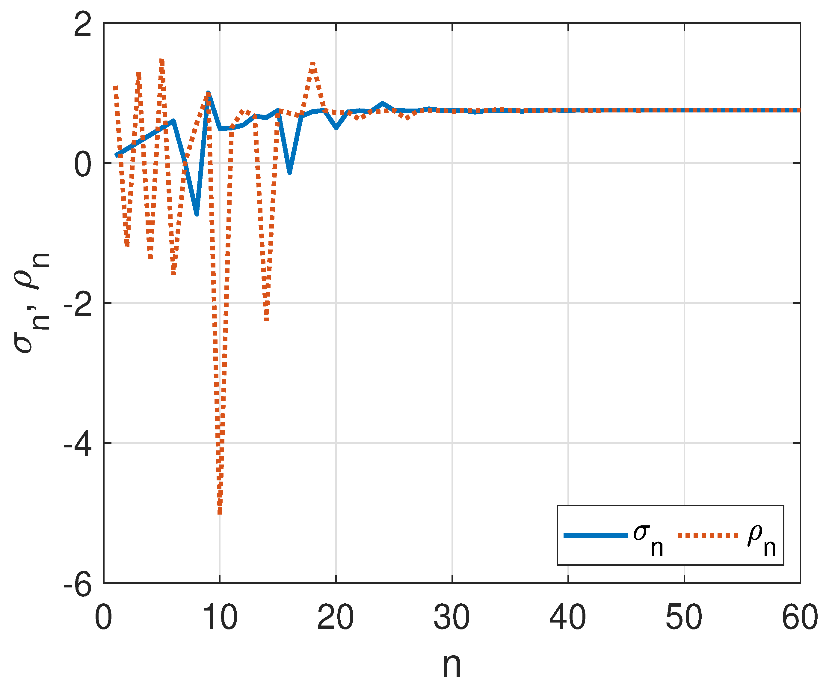
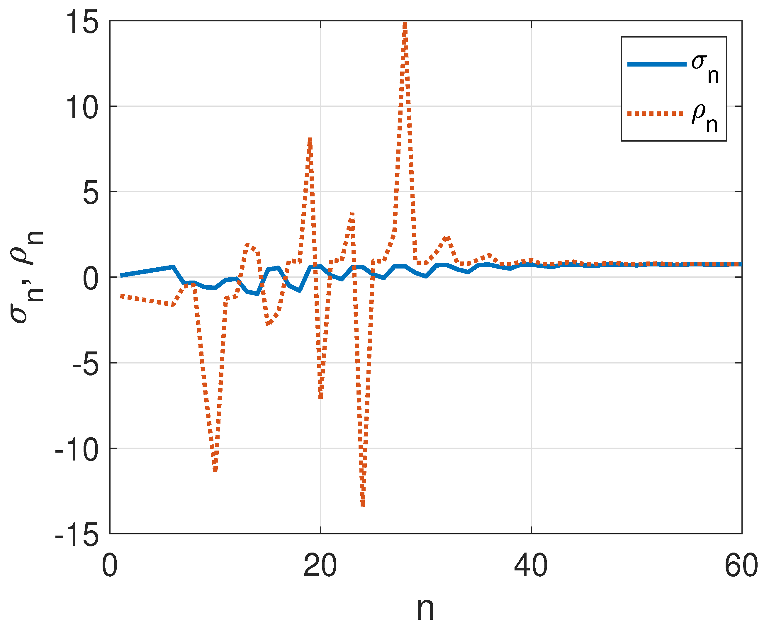
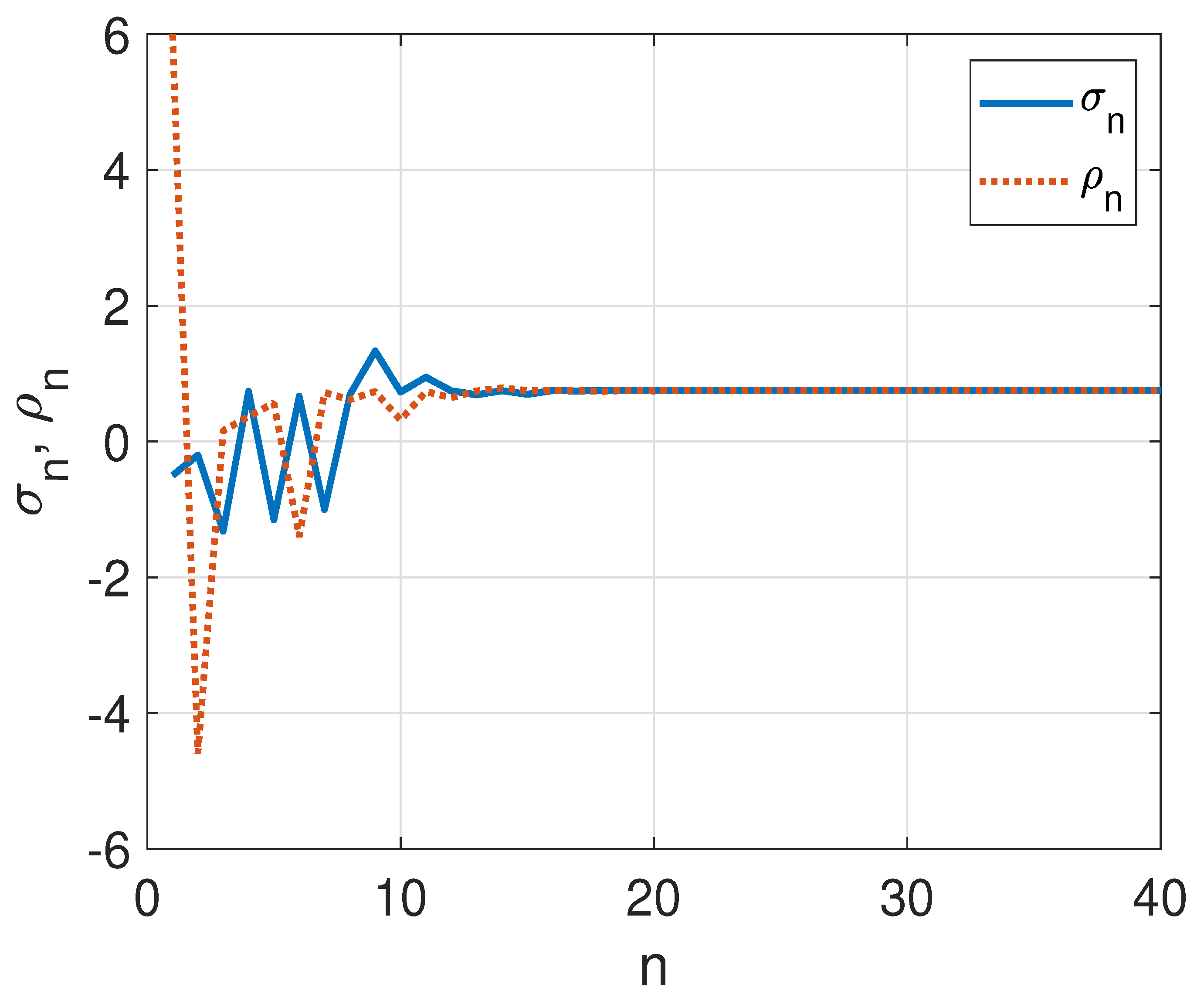
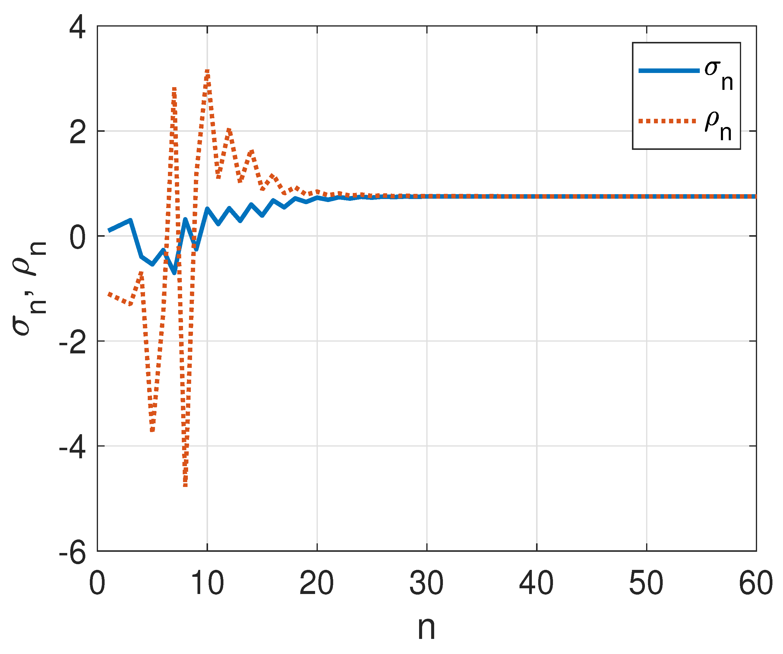
3. Illustrative Numerical Simulations

To clarify and corroborate the theoretical findings from the previous section, we delve into several compelling illustrative numerical simulations in this section.

Example 1. 

Figure 1 provides a visual representation of the sustained dynamics within System (1). The system is initialized with the conditions ${\sigma }_{-2}=-0.5$, ${\sigma }_{-1}=-0.2$, ${\sigma }_0=-1.32$, ${\rho }_{-2}=6$, ${\rho }_{-1}=-4.6$, and ${\rho }_0=0.16$.

Example 2. 

Figure 2 provides a visual representation of the sustained dynamics within System (2) for the case of $q=1$. The system is initialized with the conditions ${\sigma }_{-j}={\displaystyle \frac{1+j}{10}}$, ${\left(-1\right)}^j{\rho }_{-j}={\sigma }_{-j}+1$ for $j\in \left\{0,1,2,3,4,5\right\}$.

Example 3. 

Figure 3 provides a visual representation of the sustained dynamics within system (3). The system is initialized with the conditions ${\sigma }_{-2}=0.1$, ${\sigma }_{-1}=0.2$, ${\sigma }_0=0.3$, ${\rho }_{-2}=-1.1$, ${\rho }_{-1}=-1.2$, and ${\rho }_0=-1.3$.

Example 4. 

Figure 4 provides a visual representation of the sustained dynamics within System (4) for the case of $q=1$. The system is initialized with the conditions ${\sigma }_{-j}={\displaystyle \frac{1+j}{10}}$, and ${\rho }_{-j}=-{\sigma }_{-j}-1$ for $j\in \left\{0,1,2,3,4,5\right\}$.

Example 5. 

Figure 5 provides a visual representation of the sustained dynamics within System (4) for the case of $q=2$. The system is initialized with the conditions

j	0	1	2	3	4	5	6	7	8
${\sigma }_{-j}$	$111/3$	$125/31$	$19/2$	$127/34$	$153/15$	$139/36$	$332/7$	$341/28$	$56/17$
${\rho }_{-j}$	$-11$	$-12$	13	$-14$	15	$-16$	31	$0.24$	$0.23$

4. Conclusions

This paper presents a comprehensive investigation into fractional bidimensional systems of difference equations with higher-order terms, aiming to derive analytical expressions for their solutions under specific parametric conditions. Additionally, formulations of solutions for one-dimensional equations derived from these systems are explored. Rigorous proofs are provided for the local stability of the unique positive equilibrium point of the proposed systems. The theoretical framework established in this study is supported by extensive stability analyses and numerical simulations, which offer valuable insights into the behavior of nonlinear systems of difference equations. Notably, investigating positive equilibrium points and establishing local asymptotic stability for specific systems demonstrate the depth of our understanding. Furthermore, numerical examples using MATLAB are employed to validate the theoretical findings. Graphical illustrations of the results showcase the practical implications of the theoretical insights, reaffirming the stability of the studied systems. However, challenges persist, particularly regarding systems dynamics in unexplored scenarios. This highlights the need for continued research and exploration in this area. This paper lays a robust foundation for future investigations into more complex models, particularly those addressing dynamic systems with non-constant or periodic coefficients. Moreover, it offers avenues for broader applications and potential extensions to various scientific and engineering disciplines.

References

1. Ghezal, A.; Zemmouri, I. On Markov-switching asymmetric logGARCH models: Stationarity and estimation. Filomat 2023, 37, 1–19. [Google Scholar]
2. Ghezal, A. Spectral representation of Markov-switching bilinear processes. São Paulo J. Math. Sci. 2023, 1–21. [Google Scholar] [CrossRef]
3. Khan, A.Q.; Tasneem, M.; Younis, B.; Ibrahim, T.F. Dynamical analysis of a discrete-time COVID-19 epidemic model. Math. Meth. Appl. Sci. 2022, 46, 4789–4814. [Google Scholar] [CrossRef] [PubMed]
4. Khaliq, A.; Mustafa, I.; Ibrahim, T.F.; Osman, W.M.; Al-Sinan, B.R.; Dawood, A.A.; Juma, M.Y. Stability and bifurcation analysis of fifth-order nonlinear fractional difference equation. Fractal Fract. 2023, 7, 113. [Google Scholar] [CrossRef]
5. Al-Khedhairi, A.; Elsadany, A.A.; Elsonbaty, A. On the dynamics of a discrete fractional-order cournot–bertrand competition duopoly game. Math. Probl. Eng. 2022, 2022, 8249215. [Google Scholar] [CrossRef]
6. Abo-Zeid, R.; Cinar, C. Global behavior of the difference equation xn+1=Axn−1BCxnxn−2. Bol. Sociedade Parana. Matemática 2013, 31, 43–49. [Google Scholar] [CrossRef]
7. Berkal, M.; Abo-Zeid, R. On a rational (p + 1)th order difference equation with quadratic term. Univers. J. Math. Appl. 2022, 5, 136–144. [Google Scholar] [CrossRef]
8. Elsayed, E.M.; Alofi, B.S. The periodic nature and expression on solutions of some rational systems of difference equations. Alex. Eng. J. 2023, 74, 269–283. [Google Scholar] [CrossRef]
9. Elsayed, E.M.; Alshareef, A.; Alzahrani, F. Qualitative behavior and solution of a system of three-dimensional rational difference equations. Math. Methods Appl. Sci. 2022, 45, 5456–5470. [Google Scholar] [CrossRef]
10. Elsayed, E.M.; Aloufi, B.S.; Moaaz, O. The behavior and structures of solution of fifth-order rational recursive sequence. Symmetry 2022, 14, 641. [Google Scholar] [CrossRef]
11. Elsayed, E.M. Solution and attractivity for a rational recursive sequence. Discret. Dyn. Nat. Soc. 2011, 2011, 982309. [Google Scholar] [CrossRef]
12. Ghezal, A. Note on a rational system of (4k + 4)-order difference equations: Periodic solution and convergence. J. Appl. Math. Comput. 2023, 69, 2207–2215. [Google Scholar] [CrossRef]
13. Kara, M. Investigation of the global dynamics of two exponential-form difference equations systems. Electron. Res. Arch. 2023, 31, 6697–6724. [Google Scholar] [CrossRef]
14. Elsayed, E.M.; Alshabi, K.N. The dynamical behaviour of solutions for nonlinear systems of rational difference equations. Res. Commun. Math. Math. Sci. 2023, 15, 1–20. [Google Scholar]
15. Al-Basyouni, K.S.; Elsayed, E.M. On some solvable systems of some rational difference equations of third order. Mathematics 2023, 11, 1047. [Google Scholar] [CrossRef]
16. Okumuş, İ.; Soykan, Y. On the solutions of systems of difference equations via Tribonacci numbers. arXiv 2019, arXiv:1906.09987. [Google Scholar] [CrossRef]
17. Abo-Zeid, R. Global behavior of two third order rational difference equations with quadratic terms. Math. Slovaca 2019, 69, 147–158. [Google Scholar] [CrossRef]
18. Simşek, D.; Oğul, B.; Çınar, C. Solution of the rational difference equation xn+1=xn−17/1+xn−5.xn−11. Filomat 2019, 33, 1353–1359. [Google Scholar] [CrossRef]
19. Ghezal, A.; Zemmouri, I. On a solvable p-dimensional system of nonlinear difference equations. J. Math. Comput. 2022, 12, 195. [Google Scholar]
Figure 1. Dynamics exhibited by a specific solution of System (1).
Mathematics 12 01159 g001
Figure 2. Dynamics exhibited by a specific solution of System (2).
Mathematics 12 01159 g002
Figure 3. Dynamics exhibited by a specific solution of System (3).
Mathematics 12 01159 g003
Figure 4. Dynamics exhibited by a specific solution of System (4).
Mathematics 12 01159 g004
Figure 5. Dynamics exhibited by a specific solution of System (4).
Mathematics 12 01159 g005
Disclaimer/Publisher’s Note: The statements, opinions and data contained in all publications are solely those of the individual author(s) and contributor(s) and not of MDPI and/or the editor(s). MDPI and/or the editor(s) disclaim responsibility for any injury to people or property resulting from any ideas, methods, instructions or products referred to in the content.