Abstract
This study investigates coordinated behaviors and the underlying collective intelligence in biological groups, particularly those led by informed leaders. By establishing new convergence condition based on experiments involving real biological groups, this research introduces the concept of a volitional term and heterogeneous networks, constructing a coupled-force Cucker–Smale model with informed leaders. Incorporating informed leaders into the leader-follower group model enables a more accurate representation of biological group behaviors. The paper then extracts the Flock Leadership Hierarchy Network (FLH), a model reflecting real biological interactions. Employing time slicing and rolling time windows, the study methodically analyzes group behavior stages, using volatility and convergence time as metrics to examine the relationship between group consistency and interactions. Comparative experiments show the FLH network’s superior performance. The Kolmogorov-Smirnov test demonstrates that the FLH network conforms to a power-law distribution, a prevalent law in nature. This result further illuminates the crucial role that power-law distribution plays in the evolutionary processes of biological communities. This study offers new perspectives on the evolution of biological groups, contributing to our understanding of the behaviors of both natural and artificial systems, such as animal migration and autonomous drone operations.
Keywords:
coordinated behavior; informed leaders; group consistency; biological interaction; power-law distribution; complex network MSC:
92C42
1. Introduction
Coordinated consistency in biological groups, a universal phenomenon in nature, highlights the importance of interaction patterns between individuals alongside their inherent characteristics [1,2]. This phenomenon is evident in the high degree of synchrony and coordination of individual actions within groups, allowing organisms to adapt effectively to environmental changes, optimize foraging efficiency, and maintain social structure stability. For instance, fish schools evade predators through coordinated swimming [3,4], and migratory bird communities utilize synchronized flights for long-distance migration [5]. Similarly, bee and ant societies maintain their complex social structures through coordinated behaviors [6]. Studying coordinated consistency in biological groups has significant implications, enhancing our understanding of biology and ecology [7] and contributing to advancements in engineering [8], physics [9], biology [10,11], and social sciences [12].
A key question in studying coordinated consistency in biological groups is understanding the group’s decision-making mechanisms, such as choosing destinations, paths, and departure times. Current insights into group decision making stem from two primary perspectives. The first suggests that decision making is distributed among all group members who adhere to the established rules [13]. Typically, individuals modify their decisions based on interactions with those near them, leading to a collective compromise on routes. Research indicates [14] that this compromise strategy particularly suits animal groups with limited information-processing capabilities. However, it can result in inefficiencies, ambiguous responsibilities, and reduced adaptability. The second perspective posits that decision making in certain advanced animal groups is concentrated among a few leaders with critical information [13]. For instance, a distinct hierarchy is evident in pigeon colony flights [15,16]. Once established, these leadership structures are resilient to change, unless leaders receive misleading external information [17,18]. Therefore, the efficiency and effectiveness of group decision making are influenced by factors such as information availability, group structure, and inter-individual interactions, offering significant insights into biological group behaviors and decision-making processes.
Leadership power within groups can be classified into two main categories [19]: structured leaders and informed leaders. Informed leaders are established when a subset of the group possesses crucial information and acts upon it [20,21]. For instance, during caribou migration, experienced individuals lead the way, while others react to local food availability and predation threats. Similarly, in elephant herds, typically the older, more experienced female elephants guide the group to essential resources like water, food, and safe habitats that are vital for the group’s survival and reproduction. In mathematical models, defining informed leaders and applying network science to uncover their underlying principles remains a challenging and active area of research.
Research on modeling group systems in biology dates back to the 1980s. The biologist Reynolds [1] proposed three fundamental behaviors for natural biological groups: separation, alignment, and cohesion. Subsequent advancements in this field include Vicsek’s renowned multi-particle model, which illustrates the synchronized motion of an autonomous system comprising multiple particles [22]. This model demonstrated, through simulations, that particle synchronization is achievable with minimal external interference. Moreover, Jadbabaie [23] provided a theoretically rigorous proof of the conditions necessary for velocity synchronization in the Vicsek model. Cucker [24] explored particle swarms with Newtonian interactions, quantifying the influence between individuals by their distances and adjusting velocities based on a weighted average of velocity differences. This led to the development of the influential Cucker–Smale (CS) population model. Recent studies have delved into more intricate and realistic dynamics, such as molecular physics [25], local interactions [26], predator–prey [27], and metric distance models [28,29]. Despite discussions of hierarchical relationships in the literature, most simulations assume an equal status among individuals. Research from the perspective of informed leadership in group behaviors remains relatively unexplored.
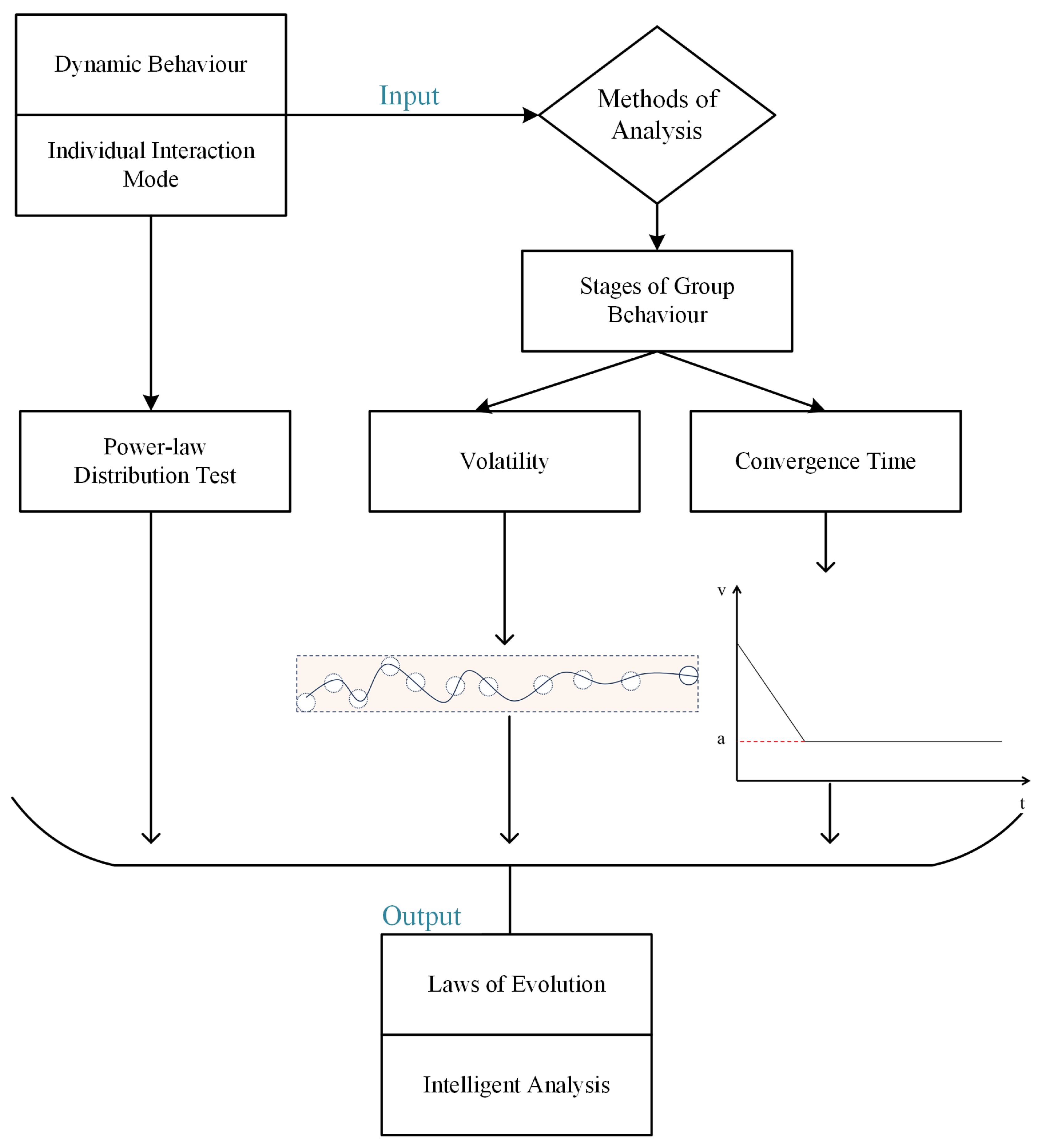
This study focuses on collective biological behavior involving informed leaders, incorporating inter-particle coupling forces into the CS model to realize the heterogeneous properties of the group. Furthermore, a resource attraction term is introduced for informed leaders, allowing for a more precise characterization of the group’s dynamic behavior, thereby enhancing our understanding of biological collectives with informed leadership. Subsequently, inspired by the topological structure of pigeon flocks, we propose the FLH interaction model generation algorithm, which accurately extracts the real interaction patterns of pigeon flocks. Statistical tests demonstrate that the degree distribution of the FLH interaction model follows a power-law distribution. By combining the FLH with other common interaction models, we employ rolling time windows and time slices to divide collective behavior into different phases, and evaluate the various interaction models based on group volatility and convergence time. Comparative experiments indicate that models using the FLH interaction as input exhibit superior metric performance, indirectly revealing the wisdom of biological collectives. The article’s framework is illustrated in Figure 1.
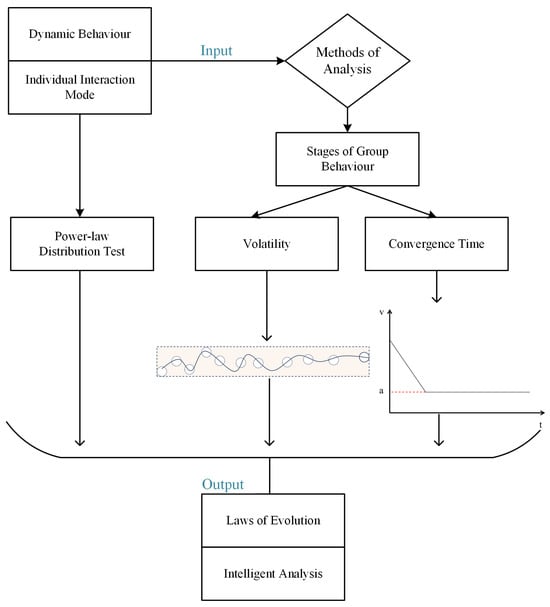
Figure 1.
Article framework. a is a certain constant.
2. Materials and Methods
2.1. Group Dynamics Models
2.1.1. Group Dynamics Model with Coupling Forces
In simulating natural group dynamics, developing artificial intelligence systems, and analyzing social behavior dynamics, the CS group model plays a pivotal role. The traditional CS model is based on the following assumptions [30]:
- (1)
- Homogeneity: The model presupposes that all individuals within the system exhibit uniform behavior, adhering to a common set of rules for updating their states. Specifically, each individual adjusts its velocity by calculating the weighted average of velocity differences with other individuals.
- (2)
- Local Interactions: Updates to an individual’s motion state are contingent upon the states of its immediate neighbors. This mechanism is consistent with the phenomenon of information transmission through visual, auditory, or other sensory means among natural groups such as flocks of birds and schools of fish.
- (3)
- Neglecting Environmental Influences: The model does not directly incorporate the impact of environmental factors on the motion states of individuals.
- (4)
- Harmonic Interactions: The interaction force between individuals diminishes with increasing distance, with this force being designed to facilitate cohesive and coordinated behavior within the group.
The CS model is characterized by its wide applicability, realistic depictions of interactions, and rigorous mathematical analysis, making it a crucial tool for studying complex group behaviors. The specifics of the model are described as follows [30]:
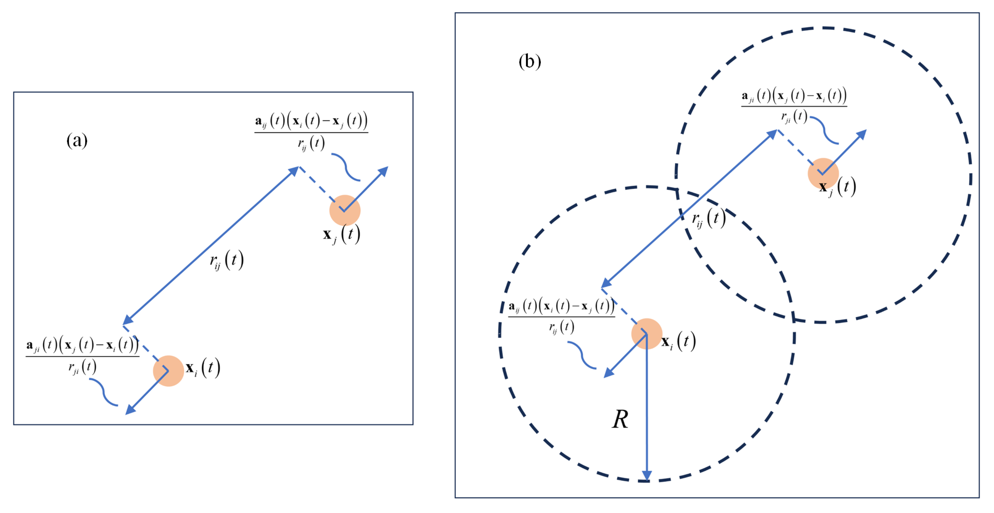
where denotes time. represent the individuals i and j, respectively. represent the positions of i and j, respectively. is the communication rate between individuals, which depends on the square of the Euclidean distance between two individuals i and j, denoted as (see Figure 2a). signifies the coordination parameter, which determines whether the communication rate is long-ranged or short-ranged. An increase in results in a more rapid diminution of the influence between individuals as the distance between them increases. The first differential equation in Equation (1) employs a fundamental form of Newton’s laws of motion, delineating that the rate of change in the position of individual i, equals its velocity vector . The second differential equation in Equation (1) reveals how evolves over time t. This evolution is determined by the weighted average influence of all other individuals in the group on individual i. When the velocity of another individual j exceeds that of individual i, individual i will attempt to accelerate to match the average velocity of the group, and vice versa. Here, is a positive constant representing the strength of the coupling effect between individuals, while N denotes the total number of individuals in the group. The interaction mechanism is weighted by the interaction function , ensuring that individuals in closer proximity exert a more significant influence on i.
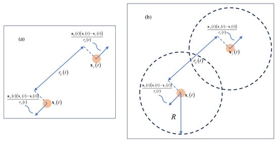
Figure 2.
(a) illustrates the pairwise acceleration between individuals, denoted as , which represents the acceleration of individual i due to the action of individual j. The direction of follows the unit vector , showing the interaction between the two entities. In (b), each individual calculates its acceleration so that and the relative velocity between the two agents converges to zero when .
We first recall the definition of asymptotic flocking, as described in Definition 1.
Definition 1
([31]). For the biological group model , certain conditions must be simultaneously met to guarantee asymptotic flocking, considering all individuals :
- (1)
- Velocity Alignment: The model’s velocity should achieve asymptotic consistency over time.
- (2)
- Group Formation: At any given moment t, the distances between individuals in the system remain finite.
Additionally, the literature [30] imposes the following constraints on and . Equation (1) attains asymptotic flocking under any of the following conditions:
Park [32] introduced the concept of inter-particle coupling forces to the CS model (IpCf-CS), ensuring collisions are avoided while allowing the system to achieve a more stringent equilibrium configuration, thereby resulting in a tighter arrangement among individuals. The system incorporating coupling forces is described as follows:
The above system has been improved upon based on the foundation of Equation (1). Herein, the positive constant represents the coupling strength of the cohesive force among individuals, and K is a designated positive gain. R is defined as the maximum communication radius between individuals (see Figure 2b). This extended CS model provides a framework capable of describing more complex group dynamics, making it more suitable for studying and understanding collective behaviors in biological groups, such as the flight formations of birds and swimming patterns of fish.
2.1.2. Biological Group Model with Informed Leaders
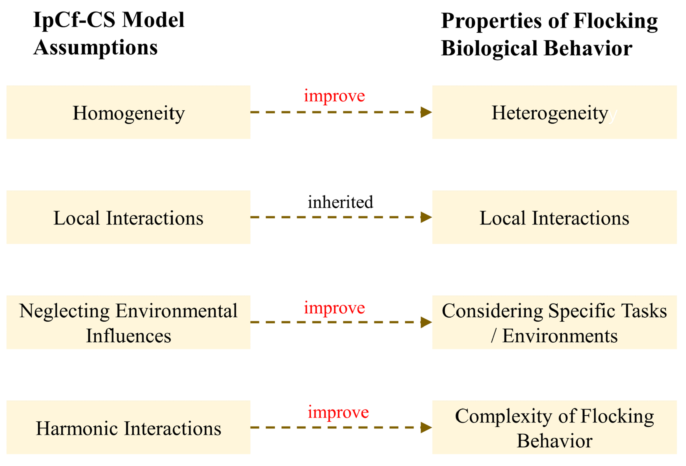
In real biological group systems, the foundational assumptions of the IpCf-CS model are overly idealized, primarily manifested in three aspects: First, although treating individuals within a group as homogeneous simplifies the analysis, the reality of internal differences within biological groups (such as age, gender, health status, etc.) significantly impacts their behavior. Secondly, under specific environmental conditions, the influence of environmental factors (e.g., food distribution, predator threats, etc.) on the movement of biological groups cannot be overlooked. Lastly, while the IpCf-CS model can portray some basic group behavior patterns, such as alignment and cohesion, biological groups often exhibit more complex patterns involving leadership-following mechanisms and decision-making processes. Therefore, this section extends these foundational assumptions by introducing the concept of informed leaders commonly present in biological group behavior (see Figure 3).
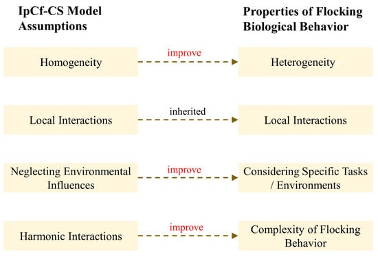
Figure 3.
Schematic illustration of the extension of assumptions about biological group behaviors.
Acknowledging the impracticality of individuals s being infinitely distant and still interacting with each other in realistic biological motion, we refine Section 2.1.1 in Definition 1. An anti-collision upper limit, denoted as , is introduced. For interaction and subsequent asymptotic flocking to occur, the distance between individuals in the system must be less than at any given moment t.
Dong [33] considered a group with a leader, where leader agent 0 possesses a free-will acceleration . For followers with a set of leaders , the behavior of a flock with a free-will leader is described by the following model:
where represents the adjacency matrix for individual interactions, with indicating an interaction between i and j, and indicating no interaction between i and j.
Within the framework of Equation (7), the leader is depicted as being entirely uninfluenced by the followers, a concept that is mathematically plausible. However, in the realm of actual biological behaviors, the leader-follower structure is not always unidirectional. That is, leaders not only influence followers, but followers can also impact leaders. For instance, when an elder matriarch elephant leads the herd in search of water or food, should a calf fall behind due to fatigue or other reasons, the entire group may slow down or change direction to protect the calf. Similarly, in avian flock flight, other birds in the group adjust their positions and flight speeds in response to changes initiated by the lead bird and surrounding environmental shifts. This feedback loop ensures that the entire group migrates efficiently.
Given this, improvements have been made under the framework of Equation (7) to make the model more closely mirror authentic collective biological behaviors. Moreover, within this enhanced framework, informed leaders are introduced into Equation (8):
where i denotes the informed leader, with L representing the set of informed leaders. The scalar form of the position of node i is denoted by . j is a follower, with F denoting the set of followers. Concurrently, we have added a unique volitional term for the informed leaders, indicating that the informed leaders are aware of the target point D location and will formulate corresponding action routes, implying an attraction to D. This attraction is modulated by an exponential function, enhancing the attraction as the distance between the individual and the target point increases. This design aims to simulate the natural response of individuals attracted by distant targets and how they adjust their movement direction and speed towards the target. To prevent individuals from breaking away from the flocking system due to excessive velocity or acceleration, Equation (8) establishes upper limits for the velocity and acceleration of each individual, denoted as and , respectively. Such constraints better reflect the behavior of a realistic biological population, where individual speed and acceleration are not infinite. Additionally, an anti-collision range is set to minimize collisions between individuals.
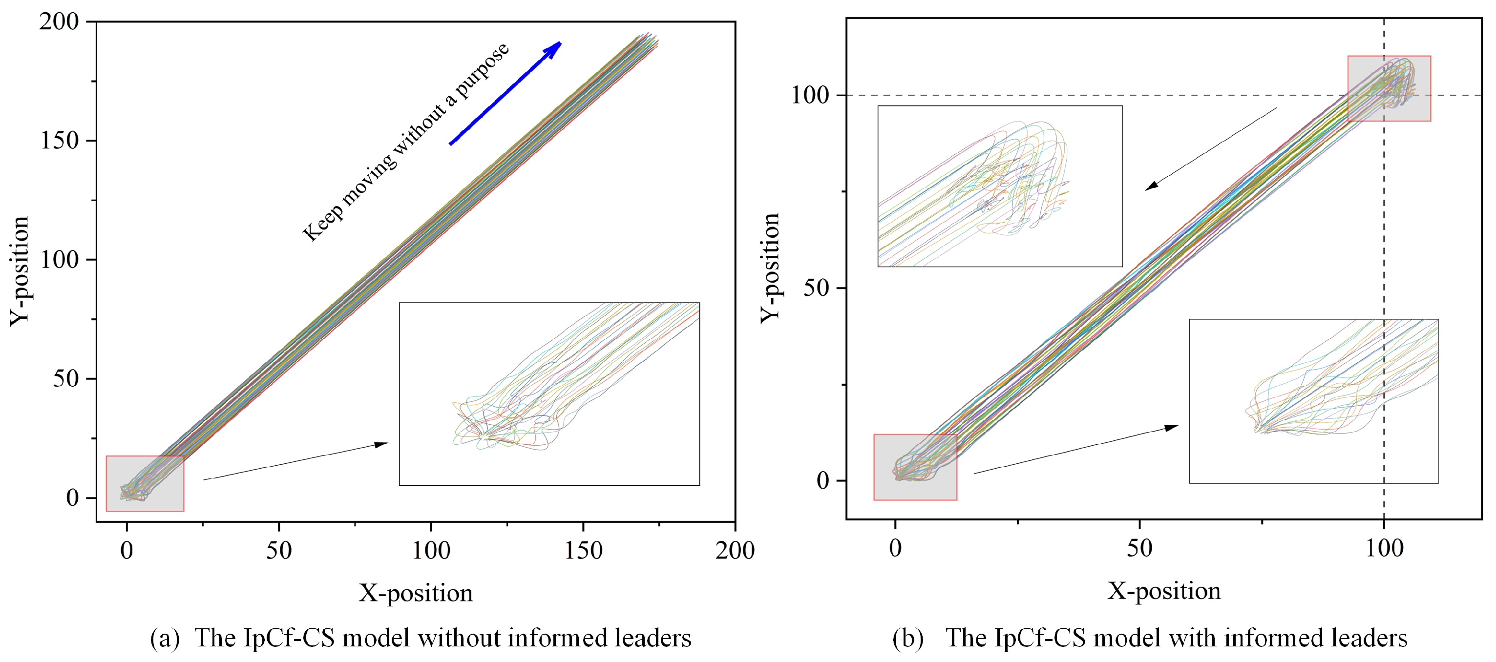
The enhancement allows for more effective information flow control within the group, improves overall system performance, and facilitates more accurate simulations of intelligent group behavior. To distinctly compare the IpCf-CS model without informed leaders (Equation (5)) and the IpCf-CS model with informed leaders (Equation (8)), Figure 4 illustrates the positional changes in the group model before and after its improvement.
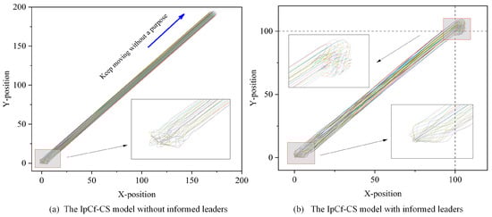
Figure 4.
Model comparison figure. Using the same model parameters, (a) displays the behavioral trajectories of all individuals strictly following the rules outlined in Equation (5). Different colors represent different individuals. However, when the model is modified to include at least one informed leader, that is, when some individuals as introduced as informed leaders (following the rules of Equation (8)) while the rest of the individuals continue to move dynamically according to the rules of Equation (5), the corresponding behavioral trajectories are depicted in (b). In both cases, the horizontal and vertical axes of (a,b) represent the X- and Y-positional coordinates of each individual, respectively. A detailed examination of (a) near the origin shows that the velocities, directions, and positions of the individuals are initially random, indicating the unpredictability of their starting states. Over time, this randomness gives way to a gradual stabilization of the group, leading to consistent behavior. In the absence of an informed leader, the group exhibits a uniform motion pattern, maintaining almost constant speed and direction. Conversely, (b), with the informed leader’s destination set at , presents a different scenario. A closer look reveals that the group ceases movement as it approaches the set destination, in contrast to the continuous motion observed in (a).
Figure 4 demonstrates the effects of introducing an informed leader into the group dynamics. This addition not only directs the group towards a specific objective but also enables the group to halt upon reaching the target location. The enhanced model offers significant insights into the dynamics of group behavior, highlighting the influential role of an informed leader.
2.2. Individual Interaction Mode
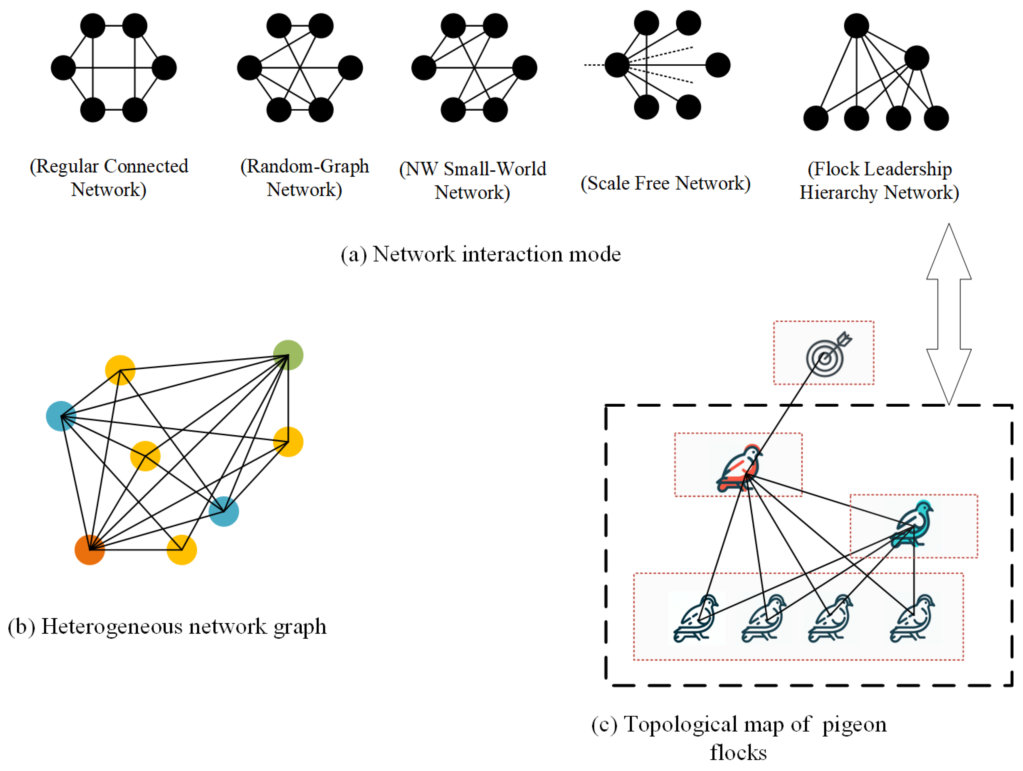
Individual interaction modes are pivotal in shaping group behavior. Within interaction networks, individuals are typically represented as nodes, and the relational roles between them are depicted through connecting edges. Currently, modeling the interaction relationships within biological groups is commonly carried out using several models, including Regularly Connected Networks, Random Graph Networks, Small-World Networks, and Scale-Free Networks [34]. This section introduces four widely recognized interactive mode generation models [35]. Concurrently, the Flock Leadership Hierarchy Network, inspired by pigeon flocking interaction patterns, aims to model and analyze group behaviors in biology. This approach is particularly relevant to scenarios involving bird groups or other animals led by a hierarchically structured leader. Figure 5 presents a schematic representation of the topology based on five interactive mode generation rules.
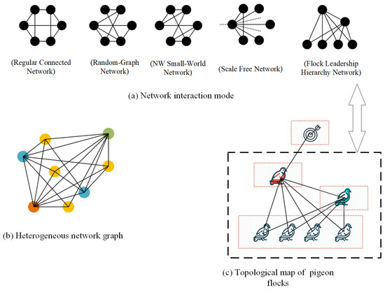
Figure 5.
Network Topology and Heterogeneous Networks. (a) illustrates the interaction patterns generated from six nodes and nine connected edges using various network generation models. Notably, in SF model representation, dashed lines signify connections to nodes external to the six depicted in the figure. (b) presents a schematic of a heterogeneous network, where nodes of different types are indicated by distinct colors. (c) serves as an example of modeling a pigeon flock through a heterogeneous network. In this model, nodes at different hierarchical levels exhibit different dynamic behaviors and are thus represented as distinct node types.
2.2.1. Regular Connected Networks (RC)
RC networks are widely observed and easily identifiable in both human society and the natural world. For instance, in the field of physics, various crystal structures serve as exemplary cases of regular networks [36], where atoms or molecules are arranged in a highly ordered manner within three-dimensional space. Similarly, in biological structures, such as the hexagonal arrangement of honeycombs [37], can be considered as two-dimensional regular networks. Such arrangements not only maximize the efficiency of space utilization but also enhance structural stability. Hence, despite their highly ordered structure, RC networks are crucial to our understanding of the inherent properties and behavioral patterns of specific systems. Nodes in regular networks exhibit specific patterns, with a common example being networks where each node has an identical degree, signifying an equal number of outward connections for every node. The generation of an RC network involves the following steps:
- (1)
- Initialization: Begin with N isolated nodes.
- (2)
- Connection Process: For each node i (where ), establish sequential connections to a set j of E target nodes. To maintain the network’s regularity and ensure that connections loop back as they reach the end of the j list, the target nodes are determined using the modulo operation (where ). The resulting network contains a total of edges.
2.2.2. Random Graph Networks (RG)
RG networks have seen extensive application in both social and natural realms. For instance, in social networks, the relationships and interactions among individuals often exhibit characteristics of random connections, appearing to be randomly established [38]. Similarly, in ecosystems, the interaction networks among species demonstrate randomness [39]. RG networks, due to their capacity to capture the randomness and complexity within systems, have become an indispensable tool in researching issues within social and natural sciences. By analyzing the structure and dynamics of random networks, scientists are better equipped to understand the behaviors and patterns of complex systems, thus providing a solid scientific foundation for predicting and managing these systems. In an RG network, edges are established randomly, without adherence to any specific rule or pattern. Such networks are commonly employed as benchmarks in real-world network analyses, serving as an exemplar of an idealized network structure. The generation of an RG network proceeds as follows:
- (1)
- Initialization: Begin with N isolated nodes.
- (2)
- Connection Process: Consider all distinct node pairs, denoted by i and , exactly once from the given N nodes. Connect each node pair with an edge at a probability . The expected number of edges in the RG network is statistically calculated as follows: .
2.2.3. Newman–Watts–Strogatz Small-World Networks (NW)
Small-world properties are commonly observed in social and ecological networks, characterized by rapid information transfer and significant performance shifts due to minor modifications in a few connections. In ecosystems, food webs exhibit characteristics of small-world networks, where species can influence each other through a few intermediary species [40]. This aspect is crucial for the stability of ecosystems and their resistance to external disturbances. Similarly, in gene regulatory networks, the regulatory relationships between genes within cells also form networks with small-world properties [41]. Such networks facilitate cells’ rapid response to environmental changes and the regulation of biological processes. The generation of an NW small-world network proceeds as follows:
- (1)
- Initial Structure: The process begins with a regular graph of N nodes. This graph forms a one-dimensional cyclic lattice, where each node connects to its nearest k neighbors, with on each side.
- (2)
- Edge Addition: For each node pair i and j in the graph, a new edge is added between them at a fixed reconnection probability p. The process prohibits the creation of multiple edges between two nodes (heavy edges) and self-loops. The resulting NW network is distinguished by short characteristic path lengths between nodes and a high clustering coefficient.
2.2.4. Scale-Free Networks (SF)
SF networks are prevalent in various domains, including physics, biology, sociology, and economics. In the domain of social networks, social media platforms such as Twitter and Facebook exhibit the characteristics of scale-free networks, where a subset of users has a vast number of followers, while the vast majority possess relatively few followers [42]. Regarding neural networks, the connections between neurons within the brain also demonstrate scale-free network traits, with a minority of neurons possessing an exceptionally high number of connections, playing a crucial role in the transmission of neural signals and the brain’s information processing capabilities [43]. The attributes of SF networks not only facilitate our understanding of complex interactions and phenomena within social and natural systems but also provide a significant theoretical foundation and practical value in designing systems resistant to interference, formulating propagation strategies, and controlling diseases. In these networks, the number of connections per node often adheres to a power-law distribution, where most nodes have few connections, but a few nodes have a significantly higher number. The process for generating an SF network is as follows:
- (1)
- Initialization: Begin with N isolated nodes.
- (2)
- Weight Assignment: Assign a weight to each node i, where and .
- (3)
- Edge Formation: Randomly select two distinct nodes i and based on probabilities proportional to their respective weights and . Add an edge from i to j (if they are not already connected).
- (4)
- Iteration: Repeat Step (3) until M edges have been established. The resulting network exhibits a power-law degree distribution , where k is the degree variable and , independent of .
2.2.5. Flock Leadership Hierarchy Networks (FLH)
Watts [44] conducted extensive experiments that uncovered hierarchical structures and informed leaders in pigeon group behavior. Motivated by these findings, we introduce the Flock Leadership Hierarchy Network (FLH), a model based on the topology of biological groups in nature. The FLH primarily explores hierarchical and leadership dynamics in group decision making, with a focus on studying complex flight formations during migration and coordinated responses to feeding and predator evasion. This network offers a novel lens for examining biological group dynamics, facilitating insights into information transfer, role allocation, and inter-individual interactions within group behaviors. The subsequent sections will detail the process of implementing the FLH network and the network generation algorithm. The complete pseudo-code is presented in Algorithm 1.
- (1)
- Initialization: Begin with the number of isolated nodes. The number of individuals per layer are determined based on the number of pigeons N observed in real pigeon flock experiments [44].
- (2)
- Node Determination: For each node j in level i, where j spans from the start index of the current level to the total number of nodes within that level, establish connections. If i is less than the total number of layers, connect node j to all nodes in higher levels .
- (3)
- Iterative Connection: Continue Step (2) until all nodes across the layers are interconnected.
This hierarchical network has applications beyond biology, extending to engineering and robotics. By leveraging insights from leadership and hierarchical structures in animal populations, it facilitates the development of more efficient and adaptable artificial systems. For instance, it can inform the design of autonomous drone swarms or robotic systems that emulate flocking behavior.
| Algorithm 1 FLH network generation algorithm |
| Input: number of individuals N, number of individuals per layer |
| Output: FLH network interaction matrix |
| //Check if the sum of individuals in layers equals N |
| if sum() is not equal to N then |
| end if |
| Error: Sum of individuals in layers must equal total number of individuals |
| //Create an adjacency matrix |
| Initialize zeros matrix |
| // Populate the FLH adjacency matrix |
| Set Current index |
| for i from 1 to length do |
| for j from Current index to do |
| //Create connections from individuals in higher layers to those in lower layers |
| if i is less than length then |
| for k from to N do |
| Set adjmatrix |
| Set adjmatrix |
| end for |
| end if |
| end for |
| Increment c by |
| end for |
In this study, the strategy for selecting informed leaders involves designating nodes with higher degree counts as leaders and those with lower degree counts as followers. This approach is underpinned by the degree distribution characteristics of the network’s nodes, influencing efficiency in information dissemination. This methodology, as noted in [45], is prevalent in real-world networks. For instance, on social media platforms, users with numerous followers (high-degree (hd) nodes) often serve as opinion leaders or influencers. Their posts rapidly reach a vast audience (comprised of low-degree (ld) nodes), potentially impacting public opinion or market trends. Similarly, in biological networks such as bird flocks or schools of fish, certain individuals assume leadership roles (hd) due to their location or behavioral traits, guiding others as followers (ld). This dynamic is vital for the group’s migratory or predator-evading activities.
The increasing recognition of the intricacies within biological group systems has led a growing number of scholars to employ complex networks for modeling and analyzing these systems. While most of the current research simplifies group systems into networks of homogeneous nodes [46,47], treating all nodes as having identical functions and attributes, this approach often overlooks the varied interactions and unique dynamic behaviors of different individual types within biological groups. To address this gap, upon establishing a selection strategy for informed leaders in groups, we introduce a heterogeneous graph [48], denoted as , comprising a set of objects V and a set of links E. This graph is further characterized by a node-type mapping function and a link-type mapping function , where and represent the sets of predefined object and link types, respectively, with . We categorize individuals in biological groups into distinct types based on their dynamic behavior and model the group systems using heterogeneous networks as illustrated in Figure 5. This approach more effectively captures the heterogeneity of nodes and the diversity of connections, thereby offering a more comprehensive and precise framework for understanding and analyzing complex population systems.
3. Model Building
3.1. Stages of Group Behavior and Demonstration
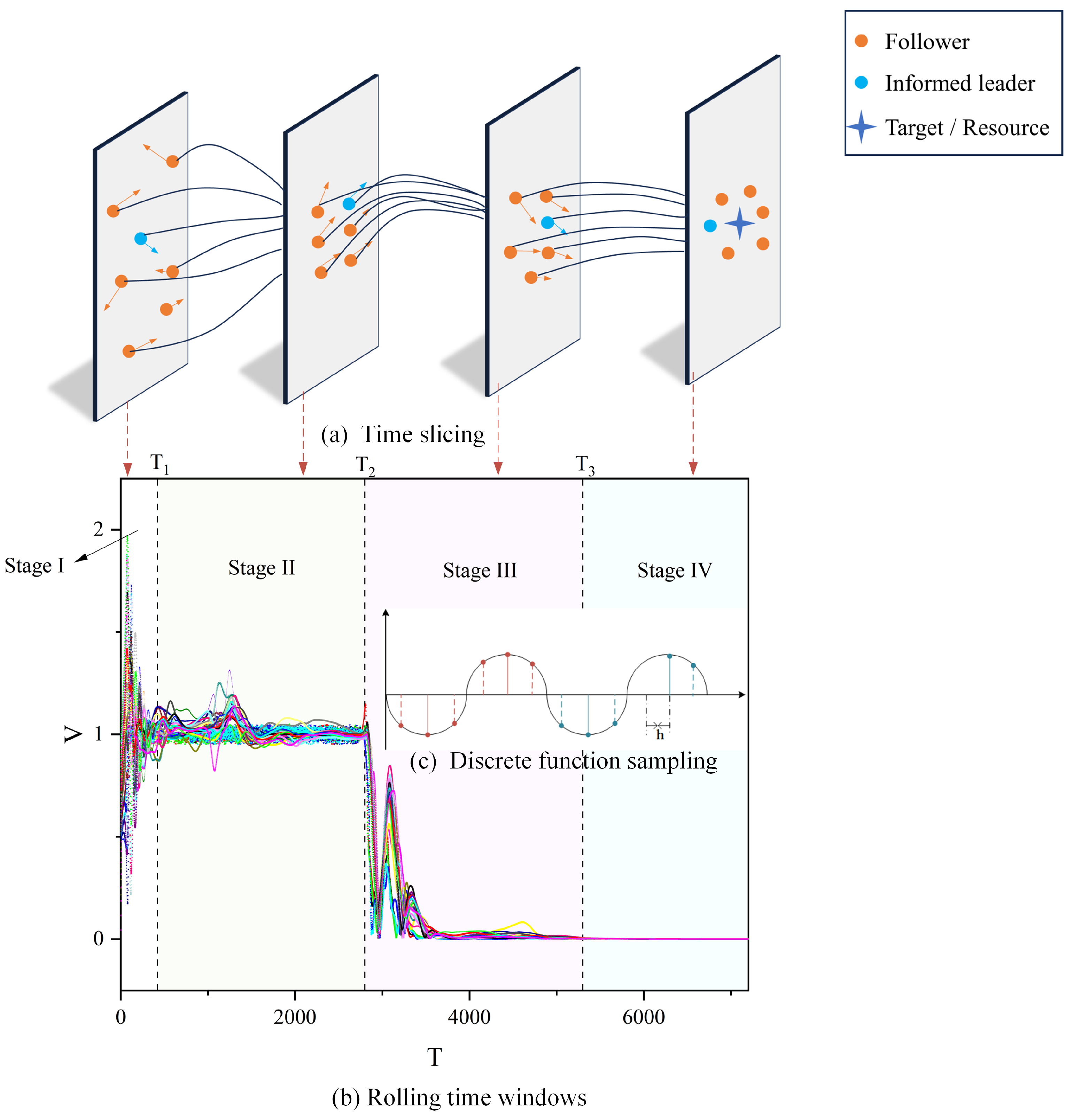
A comprehensive understanding of the various stages of group behavior is crucial for comprehending the complexities of biological systems. In the realm of biological group behaviors, such as bird flocking, fish schooling, or collective actions among insects, it is generally feasible to categorize these behaviors into four distinct phases [49]. Investigating each phase in detail significantly enhances our understanding of the dynamic characteristics of group behavior and its adaptive mechanisms. To facilitate a more precise quantitative analysis of these stages, we have implemented a uniform sampling method with a step size of for discretizing the continuous function in Equation (8), as illustrated in part (c) of Figure 6.
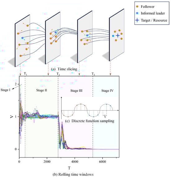
Figure 6.
Stages of group behavior (using the RC interaction model as an example). In (b), the horizontal axis T signifies the progression of time, and the vertical axis V denotes the velocity of individuals. The variously colored lines depict the trend of each individual’s velocity over time. We categorized the group’s movement into four distinct stages, each characterized by unique movement traits and represented by four different base colors. In (a), the blue circles represent informed leaders. The yellow circles represent followers. The blue four-pointed star represents the objective/resource information known to the informed leaders. Finally, the length and orientation of the arrows illustrate the magnitude and direction of their respective velocities.
In Figure 6b, the interval 0– corresponds to the initial formation stage of biological group behavior (Stage I). This phase is marked by groups beginning their movement towards a destination, exhibiting considerable variations in speed and direction, along with notable overall fluctuations. Typically, organisms start to aggregate during this phase for reasons like foraging, defense against predators, migration, etc. Analyzing Stage I is crucial for understanding the conditions initiating group behavior. The period – represents the stabilization phase of group behavior (Stage II), also referred to as the first convergence phase. Here, group motion generally fluctuates around , indicating a state of consistency akin to the uninformed leader group model. This stage, characterized by stable structures and patterns, is key to understanding social structures and information transfer within the group. The interval – denotes the decision-making phase (Stage III), where the group, led by an informed leader, heads towards its destination. As the destination nears, individual velocities decrease, and the state of motion undergoes significant changes compared to Stage II. This phase’s analysis is pivotal in uncovering group information processing and decision-making dynamics. Finally, –∞ marks the dissolution phase of group behavior (Stage IV), or the second convergence stage. In this stage, as the group, guided by an informed leader, reaches the vicinity of its destination (illustrated by a blue four-pointed star in Figure 6a), its position stabilizes, and the velocity gradually converges to zero. Dissolution in this stage may occur due to various factors, such as reaching the destination, depletion of food sources, or environmental changes. Understanding Stage IV sheds light on the ecological and social dynamics underlying group maintenance and dissolution. To visually depict each stage, we selected specific time points from Figure 6a for each stage and utilized a time-slicing approach for demonstration.
3.2. Metric Performance
3.2.1. Volatility
Volatility serves as a critical metric in analyzing biological group behavior, quantifying the extent of instability or variability in group movements [50]. Generally, a lower volatility indicates a more stable and predictable group behavior, a trait often beneficial for biological populations. In Section 3.1, we categorize stages I and III as phases of group self-adaptation, predominantly marked by groups modulating their state via fluctuations. Consequently, analyzing the volatility in these stages is not substantially relevant. Accordingly, this paper introduces the volatility indicators and to analyze stages II and IV, respectively. Due to the minimal directional variance among individuals in Stage II and IV, the dependent variable of speed in the volatility metric is represented in scalar form.
where refers to the duration of the time window under analysis. M represents the total number of intervals collected for an individual within . denotes the velocity of the jth individual at the ith time step, and is the average velocity of all individuals within . N signifies the total number of individuals.
3.2.2. Convergence Time
Convergence time is a crucial metric for assessing the efficiency with which a group achieves coherence and is paramount for understanding and evaluating group systems. In natural biological groups, a reduced convergence time is advantageous, enabling groups to more effectively escape predators or adapt to environmental changes. In light of this, this paper introduces the convergence time metrics and to denote the termination of Stages I and III, respectively. These metrics indicate the onset of convergence in Stages II and IV.
where represents the volatility of each individual within a designated time window. denotes the velocity of an arbitrary individual at the ith time step. The term signifies the end time of this time window. The volatility threshold for each individual during the specified period is denoted by . Furthermore, and c, respectively, indicate the velocity threshold and the acceptable range of volatility within the same time window.
3.3. Power-Law Distribution Test
The degree distribution of the FLH network proposed in this paper exhibits a trend similar to that observed in SF networks. Consequently, we investigate whether the FLH network’s degree distribution also adheres to a power-law distribution. This distribution is defined by , where represents the probability of nodes with degree k appearing in the network. The exponent , characterizing the power-law distribution, is typically greater than 1. C is a normalization constant ensuring that the sum of all probabilities equals 1. The exponential distribution, in contrast, is defined as , with being the rate parameter. To determine the power-law distribution index , we employ maximum likelihood estimation, as detailed in Equation (11).
where represents the estimated power-law index. The variable n denotes the number of nodes with a degree greater than or equal to . Each node’s degree is represented by , and signifies the minimum degree value to which the power-law distribution is applicable.
Subsequently, we compare the logarithmic values of the likelihood function R for the two distributions:
where the likelihood functions for the two distributions are denoted as and , respectively. A value of indicates that the power-law distribution is more appropriate than the exponential distribution, whereas suggests that the exponential distribution is a better fit. The fit’s accuracy was evaluated using the Kolmogorov–Smirnov test, which compares the cumulative distribution function of the data with the expected power-law distribution.
where and represent the empirical and theoretical values of the cumulative distribution function, respectively. In this study, the determination of is achieved by minimizing the discrepancy , where represents the maximum difference between the empirical probability distribution and the assumed power-law distribution probability . To facilitate effective comparison, we ensure that both and are normalized, thus meeting the standards of probability density functions. These functions are utilized to calculate a statistic for evaluating the disparity between the two distributions.
A statistical test is applied to ascertain the significance of this ratio, with the p-value indicating the strength of evidence against the null hypothesis, which posits that the two distributions are identical. A p-value less than 0.05 typically signifies a significant difference between the distributions, lending credibility to R; conversely, a p-value greater than 0.05 suggests that the difference is not significant, thereby questioning the reliability of R.
4. Numerical Simulation
4.1. Experimental Design
The purpose of this experiment is to evaluate the efficacy of the HLF interaction model in modeling group motion. Subsequently, the parameters within Equation (8) was configured. At time , the position of individual i is randomly generated near the point , the magnitude of the velocity is randomly generated between 0 and 1, and their initial directions are also random. Additionally, to mitigate the potential influence of network cost (namely, the number of connected edges) on the experimental outcomes, we maintained a consistent total of approximately 240 edges across the five interaction modes described in Section 2.2. The precise values of these parameters and their corresponding meanings are listed in Table 1.

Table 1.
Model parameter settings.
4.2. Discussion
In this study, we performed a range of simulation experiments using the enhanced group model outlined in Section 2.1 along with the five interaction modes. To guarantee the reliability and precision of our experimental findings, we compiled the average results from multiple experiments. Moreover, we executed several group experiments under various convergence conditions, as specified in Equation (4). Pertaining specifically to convergence condition (3) in Equation (4), the experimental outcomes are displayed in Figure 7 and Table 2.
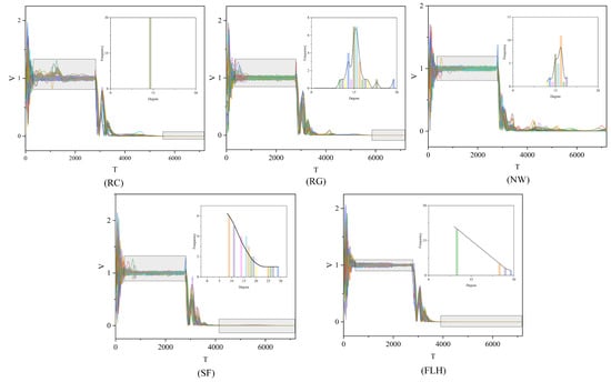
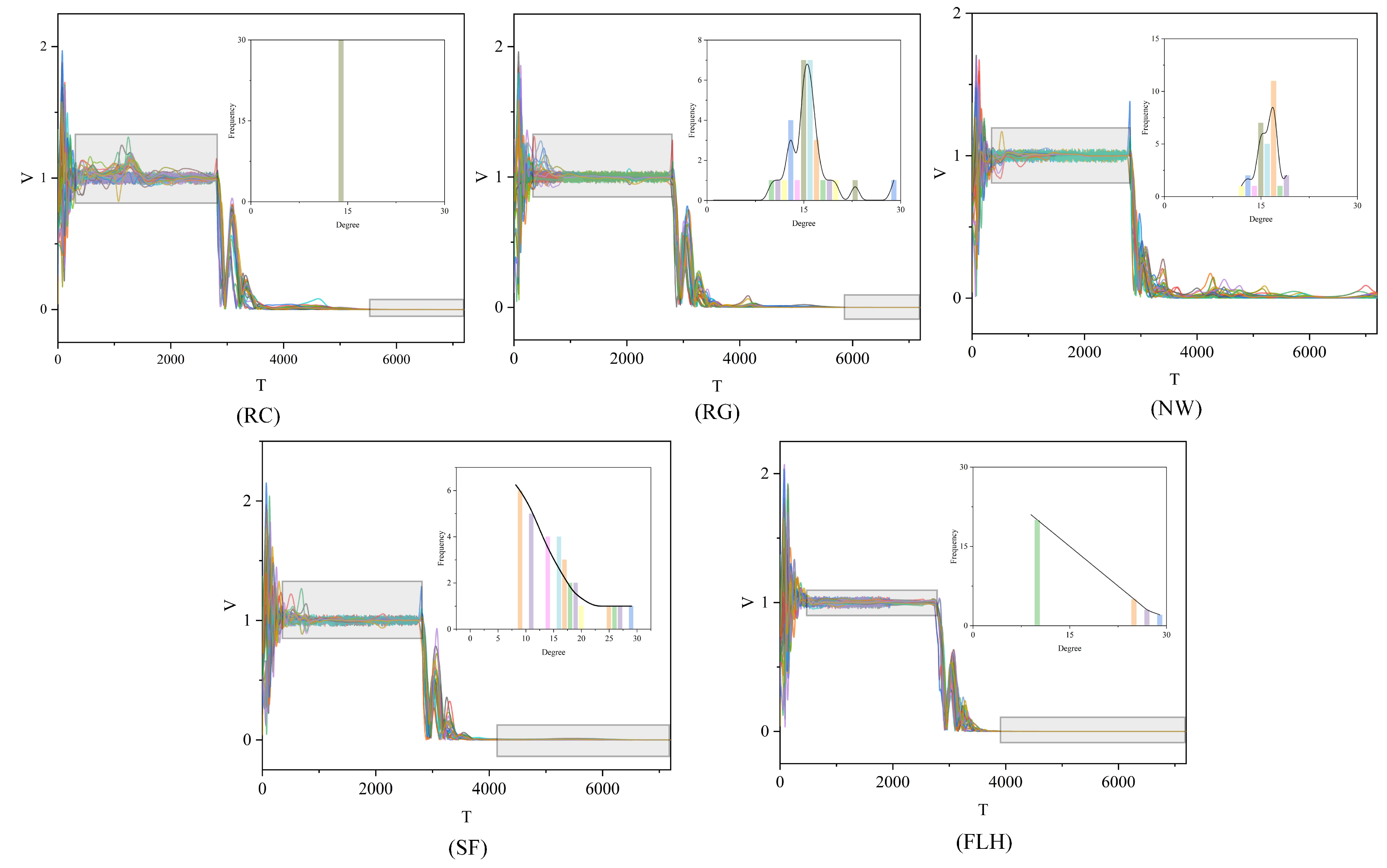
Figure 7.
Velocity figures of five group movements. The experimental results are presented in a series of graphs, each illustrating the velocity dynamics of population motion across the five interaction modes: RC, RG, NM, SF, and FLH. Different colors represent different individuals. In these graphs, the horizontal axis T depicts the progression of time, whereas the vertical axis represents the individual velocities V within the population. Accompanying subplots in each graph detail the degree distribution within the respective networks for each interaction mode. Within these subfigures, the horizontal axis denotes the degree values of the nodes, and the vertical axis shows the frequency of each degree value’s occurrence in the network. A black curve in each subplot highlights the statistical characteristics of the degree distribution.
Table 2.
The experimental results of Equation (4) (3) are obtained under the condition of consistency.
The experimental findings indicate that in the first stage, the biological group employing the FLH interaction mode achieves the shortest convergence time, recorded at . This is followed by the NW, SF, RG, and RC modes, in that order. Notably, the FLH structure demonstrates a substantial advantage in the initial convergence time, being nearly three times shorter than that of the RC mode. Regarding the convergence time in Stage III, the FLH mode continues to outperform, clocking in at , with the SF, RC, and RG modes trailing behind. The NW mode shows the least effective performance, as evidenced in Figure 7 (NW) at , where the population system still fails to meet the consistency condition of Stage IV. The individual speeds and their variances remain substantial, suggesting that the population system has not yet reached convergence. Furthermore, the experimental findings reveal that solely the SF and FLH modes conform to the power-law distribution. In conclusion, the FLH model emerges as the most advantageous approach.
For the volatility metric , the FLH network, with , exhibits the lowest volatility among the five interaction modes. In contrast, the RC network records the highest volatility in Stage II, with , markedly differing from the other networks by several orders of magnitude, as highlighted in the grey-shaded area of Figure 5 (referenced). In the case of , the FLH network maintains its superior performance in Stage IV, registering a value of . Since the NW network does not reach Stage IV within , its value remains uncalculated. The degree distribution curves of the SF and FLH networks display similar patterns, and hypothesis testing confirms that the FLH model also adheres to a power-law distribution. These two networks rank as the top performers in the group system, thereby underscoring the efficacy of power-law distributions in group behavior from both mathematical and modeling perspectives. Power-law distributions are not only prevalent in biological populations [51] but also in artificial systems such as social and Internet networks, urban systems, and natural phenomena like earthquake intensity, river lengths, and watershed areas.
The experimental outcomes for convergence conditions (2) and (1), as specified in Equation (4), are presented in Table 3 and Table 4. The data unequivocally demonstrate that the FLH interaction mode holds significant advantages over the other four interaction modes, irrespective of the settings incorporating diverse convergence parameters.
Table 3.
The experimental results of Equation (4) (2) are obtained under the condition of consistency.
Table 4.
The experimental results of Equation (4) (1) are obtained under the condition of consistency.
In the aforementioned experiments, based on the three convergence conditions proposed in Equation (4), different values of and were selected for further experimentation. These experiments confirmed that the FLH interaction mode has a significant advantage in the CS model with informed leaders. Since the FLH model is derived from real biological group interaction experiments, it further illustrates the collective intelligence exhibited by biological groups during the evolutionary process. Subsequently, to further validate the effectiveness of the model across a wide parameter range and enhance its applicability and generalizability, we fixed the parameters (, ) as specified in Table 1 as convergence conditions and conducted multiple controlled variable experiments on the collision coefficient , the maximum radius of communication R, and the number of individuals N.
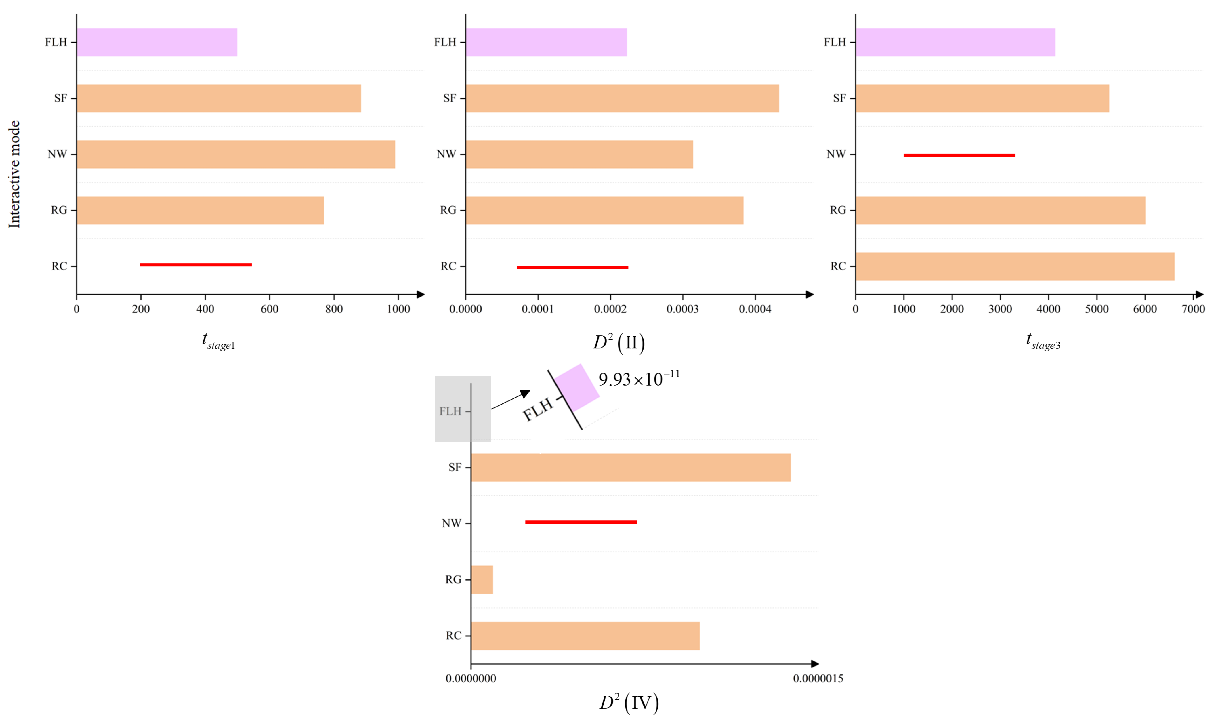
For the controlled variable experiment regarding , the collision coefficient was randomly set to in each experiment. The experimental results for the parameter are shown in Figure 8, with specific data provided in Table 5. From Figure 8, it is evident that in the experiments using multiple random settings for , the FLH network interaction mode exhibits significant advantages over the other four networks in terms of the four metrics measuring group behavior capabilities, as demonstrated by the shorter convergence times and reduced velocity fluctuations among individuals during stable stages. Therefore, the experiment indicates that within a certain range of fluctuations, any value of the collision coefficient does not affect the superior position of the FLH network interaction mode in the biological group model. This confirms the universal role of this structure in reflecting the collective intelligence of biological groups.

Figure 8.
Controlled variable experiment for the collision coefficient . The figures display the average results of network interaction modes’ performance metrics under multiple variations of the collision coefficient . In all four graphs, the y-axis represents the individual interaction modes, while the x-axis corresponds to , , , and , respectively. The pink bars represent the results of the FLH network interaction mode, orange bars represent the results of other interaction modes, and the red lines indicate instances of non-convergence in multiple experiments under that network interaction mode. Notably, in the fourth graph, due to the magnitude of the FLH mode’s advantage in volatility over other interaction modes, it is only observable through a zoomed-in view. From these graphs, it is evident that the FLH network interaction mode exhibits significant superiority across all four biological group metrics.
Table 5.
Results for the controlled variable experiment on the collision coefficient .
Similarly, for the randomly varying maximum radius of communication R, we set , with the experimental results presented in Table 6. According to the performance in within Table 6, the NW network performed best, followed by the FLH network. However, considering all four metrics, the FLH network still demonstrates a clear advantage.
Table 6.
Results for the controlled variable experiments on the maximum radius of communication R.
Given the correspondence between the number of individuals and informed leaders in real biological groups, with other parameters held constant, we defined the range of the randomly varying number of individuals as , and conducted experiments under five types of interactions. The results are shown in Table 7.
Table 7.
Results for the controlled variable experiments on the number of individuals N.
5. Conclusions
In this study, we improve the CS model by integrating coupling forces to better capture the behaviors of biological groups with informed leaders, achieving a more comprehensive portrayal of group dynamics. Additionally, we introduce the FLH network generation algorithm, inspired by the interaction patterns observed in the behaviors of pigeon flocks. The group dynamics are then segmented into four distinct phases: formation, stabilization, decision making, and dissolution. This paper also employs heterogeneous networks to model and analyze biological groups, acknowledging the diversity in nodes and their connections. We utilize two key metrics, volatility and convergence time, to assess population performance. Comparative analyses between the FLH network and four common network models reveal that the FLH-based group model excels in performance metrics and adheres to the power-law distribution, underscoring the strategic evolution of biological populations.
6. Future Research
Looking forward, the enhanced population model and network interaction patterns proposed here hold significant implications not only in biological research but also in the realms of engineering and computer science. For instance, the theoretical framework presented in this paper is highly applicable to the design of autonomous robotic behaviors and the exploration of artificial intelligence algorithms. Finally, the comprehensive description of biological group behavior stages presented in this study has substantial relevance and potential applications in developing biologically inspired algorithms and techniques. It deepens our understanding of complex biological group interactions and may foster novel approaches to modeling group behavior in natural settings. Meanwhile, as our understanding and applications of this model continue to deepen and expand, future research will focus on integrating the model with real biological group data to further validate its accuracy and practicality. By analyzing and applying a vast array of real-world data, we aim to significantly enhance the model’s predictive and generalization capabilities, making it more adaptable to real-life scenarios.
Author Contributions
Conceptualization, Y.F. and J.Z.; Methodology, Y.F. and Q.H.; Software, X.H., X.L. and X.D.; Formal analysis, J.Z.; Investigation, Y.F. and J.Z.; Resources, W.T.; Data curation, Y.F.; Writing—original draft preparation, Y.F.; Writing—review and editing, Q.H. and X.D.; Visualization, Y.F.; Supervision, X.L.; Project administration, X.D.; Funding acquisition, Q.H. All authors have read and agreed to the published version of the manuscript.
Funding
This work was supported in part by the National Natural Science Foundation of China, Grant/Award Number: 6210023156 and 12101608; the National Natural Science Foundation of China—Chinese Academy of Engineering Physics NSAF Joint Foundation, Grant/Award Number: U2230208; and the Hunan Provincial Graduate Student Research Innovation Program, Grant/Award Number: CX20230015.
Data Availability Statement
All additional data supporting the results of this study are available at: https://github.com/fuyude2022/biological-flocking-intelligence-data (accessed on 30 January 2024).
Acknowledgments
The authors thank the editor and the anonymous referees for their helpful comments and critiques.
Conflicts of Interest
The authors declare no conflicts of interest.
Abbreviations
The following abbreviations are used in this manuscript:
| CS | Cucker–Smale model |
| RC | Regular Connected Network |
| RG | Random Graph Network |
| NW | Newman–Watts–Strogatz Small-World Network |
| SF | Scale-Free Network |
| FLH | Flock Leadership Hierarchy Network |
| hd | high-degree nodes |
| ld | low-degree nodes |
| IpCf-CS | inter-particle coupling forces to the CS model |
References
- Reynolds, C.W. Flocks, Herds and Schools: A Distributed Behavior Model. ACM SIGGRAPH Comput. Graph. 1987, 21, 25–34. [Google Scholar] [CrossRef]
- Marras, S.; Killen, S.S.; Lindström, J.; Mckenzie, D.J.; Steffensen, J.F.; Domenici, P. Fish swimming in schools save energy regardless of their spatial position. Behav. Ecol. Sociobiol. 2015, 69, 219–226. [Google Scholar] [CrossRef]
- Aoki, I. A Simulation Study on the Schooling Mechanism in Fish. Nihon-Suisan-Gakkai-Shi 1982, 48, 1081–1088. [Google Scholar] [CrossRef]
- Hubbard, S.; Babak, P.; Sigurdsson, S.T.; Magnússon, K.G. A model of the formation of fish schools and migrations of fish. Ecol. Model. 2004, 174, 359–374. [Google Scholar] [CrossRef]
- Zhong, C.; Lou, W.; Lai, Y. A Projection Pursuit Dynamic Cluster Model for Tourism Safety Early Warning and Its Implications for Sustainable Tourism. Mathematics 2023, 11, 4919. [Google Scholar] [CrossRef]
- Alan, P.; Scott, T.J. Can we identify general architectural principles that impact the collective behaviour of both human and animal systems? Philos. Trans. R. Soc. B Biol. Sci. 2018, 373, 20180253. [Google Scholar]
- Huang, S.; Brangwynne, C.P.; Parker, K.K.; Ingber, D.E. Symmetry-breaking in mammalian cell cohort migration during tissue pattern formation: Role of random-walk persistence. Cell Motil. Cytoskelet. 2010, 61, 201–213. [Google Scholar] [CrossRef]
- Yaxley, K.J.; Joiner, K.F.; Abbass, H.A. Drone approach parameters leading to lower stress sheep flocking and movement: Sky shepherding. Sci. Rep. 2021, 11, 7803. [Google Scholar] [CrossRef] [PubMed]
- Hakim, V.; Silberzan, P. Collective cell migration: A physics perspective. Rep. Prog. Physics. Phys. Soc. 2017, 80, 076601. [Google Scholar] [CrossRef]
- Belmonte, J.M.; Thomas, G.L.; Brunnet, L.G.; Almeida, R.M.C.D.; Chate, H. Self-propelled particle model for cell-sorting phenomena. Phys. Rev. Lett. 2008, 100, 248702. [Google Scholar] [CrossRef]
- Rørth, P. Collective guidance of collective cell migration. Trends Cell Biol. 2007, 17, 575–579. [Google Scholar] [CrossRef] [PubMed]
- Wei, X.; Liu, J.C.; Bi, S. Uncertainty quantification and propagation of crowd behaviour effects on pedestrian-induced vibrations of footbridges. Mech. Syst. Signal Process. 2022, 167, 108557. [Google Scholar] [CrossRef]
- Smith, J.; Gavrilets, S.; Mulder, M.; Hooper, P.; Mouden, C.; Nettle, D.; Hauert, C.; Hill, K.; Perry, S.; Pusey, A. Leadership in Mammalian Societies: Emergence, Distribution, Power, and Payoff. Trends Ecol. Evol. 2015, 31, 54–66. [Google Scholar] [CrossRef] [PubMed]
- Dell’Ariccia, G.; Dell’Omo, G.; Wolfer, D.P.; Lipp, H.P. Flock flying improves pigeons’ homing: GPS track analysis of individual flyers versus small groups. Anim. Behav. 2008, 76, 1165–1172. [Google Scholar] [CrossRef]
- Nagy, M.; Akos, Z.; Biro, D.; Vicsek, T. Hierarchical group dynamics in pigeon flocks. Nature 2010, 464, 890. [Google Scholar] [CrossRef]
- Nagy, M.; Vasarhelyi, G.; Pettit, B.; Roberts-Mariani, I.; Vicsek, T.; Biro, D. Context-dependent hierarchies in pigeons. Proc. Natl. Acad. Sci. USA 2013, 110, 13049–13054. [Google Scholar] [CrossRef] [PubMed]
- Flack, A.; Ákos, Z.; Nagy, M.; Vicsek, T.; Biro, D. Robustness of flight leadership relations in pigeons. Anim. Behav. 2013, 86, 723–732. [Google Scholar] [CrossRef]
- Watts, I.; Nagy, M.; Theresa, B.D.P.; Biro, D. Misinformed leaders lose influence over pigeon flocks. Biol. Lett. 2016, 12, 20160544. [Google Scholar] [CrossRef]
- Garland, J.; Berdahl, A.M.; Sun, J.; Bollt, E.M. Anatomy of leadership in collective behaviour. Chaos 2018, 7, 5308. [Google Scholar] [CrossRef]
- Strandburg-Peshkin, A.; Twomey, C.R.; Bode, N.W.F.; Kao, A.B.; Katz, Y.; Ioannou, C.C.; Rosenthal, S.B.; Torney, C.J.; Wu, H.S.; Levin, S.A.A. Visual sensory networks and effective information transfer in animal groups. Curr. Biol. CB 2013, 23, 709–711. [Google Scholar] [CrossRef]
- Reebs, S.G. Can a minority of informed leaders determine the foraging movements of a fish shoal? Anim. Behav. 2000, 59, 403–409. [Google Scholar] [CrossRef]
- Vicsek, T.; Czirók, A.; Ben-Jacob, E.; Cohen, I.; Shochet, O. Novel Type of Phase Transition in a System of Self-Driven Particles. Phys. Rev. Lett. 1995, 75, 1226. [Google Scholar] [CrossRef] [PubMed]
- Jadbabaie, A.; Lin, J.; Morse, A.S. Coordination of groups of mobile autonomous agents using nearest neighbor rules. IEEE Conf. Decis. Control 2002, 3, 2953–2958. [Google Scholar]
- Cucker, F.; Smale, S. Emergent behavior in flocks. IEEE Trans. Autom. Control 2007, 52, 852–862. [Google Scholar] [CrossRef]
- Tunstrøm, K. Determining interaction rules in animal swarms. Behav. Ecol. 2010, 21, 1106–1111. [Google Scholar]
- Lukeman, R.; Li, Y.X.; Edelstein-Keshet, L. Inferring individual rules from collective behavior. Proc. Natl. Acad. Sci. USA 2010, 107, 12576–12580. [Google Scholar] [CrossRef] [PubMed]
- Zhdankin, V.; Sprott, J.C. Simple predator-prey swarming model. Phys. Rev. E Stat. Nonlinear Soft Matter Phys. 2010, 82, 056209. [Google Scholar] [CrossRef]
- Couzin, I.; Krause, J.; Franks, N.; Levin, S. Effective leadership and decision-making in animal groups on the move. Nature 2005, 433, 513–516. [Google Scholar] [CrossRef]
- Guo, H.; Han, J.; Zhang, G. Hopf Bifurcation and Control for the Bioeconomic Predator–Prey Model with Square Root Functional Response and Nonlinear Prey Harvesting. Mathematics 2023, 11, 4958. [Google Scholar] [CrossRef]
- Cucker F, S.S. On the mathematics of emergence. Jpn. J. Math. 2007, 2, 197–227. [Google Scholar] [CrossRef]
- Ha, S.; Liu, J. A simple proof of the Cucker–Smale flocking dynamics and mean-field limit. Commun. Math. Sci. 2009, 7, 297–325. [Google Scholar] [CrossRef]
- Park, J.; Kim, H.; Ha, S. Cucker–Smale Flocking With Inter-Particle Bonding Forces. IEEE Trans. Autom. Control 2010, 55, 2617–2623. [Google Scholar] [CrossRef]
- Dong, J. Flocking under hierarchical leadership with a free-will leader. Int. J. Robust Nonlinear Control 2012, 23, 1891–1898. [Google Scholar] [CrossRef]
- Liang, J.; Qi, M.; Gu, K.; Liang, Y.; Zhang, Z.; Duan, X.J. The structure inference of flocking systems based on the trajectories. Chaos 2022, 32, 101103. [Google Scholar] [CrossRef]
- Chen, G.; Lou, Y.; Wang, L. A Comparative Study on Controllability Robustness of Complex Networks. IEEE Trans. Circuits Syst. II Express Briefs 2019, 66, 828–832. [Google Scholar] [CrossRef]
- Bürgi, H.B. Crystal structures. Acta Crystallogr. Sect. B Struct. Sci. Cryst. Eng. Mater. 2022, 78, 283–289. [Google Scholar] [CrossRef]
- Yin, H.; Huang, X.; Scarpa, F.; Wen, G.; Chen, Y.; Zhang, C. In-plane crashworthiness of bio-inspired hierarchical honeycombs. Compos. Struct. 2018, 192, 516–527. [Google Scholar] [CrossRef]
- Lee, S.; Cha, Y.; Han, S.; taek Hyun, C. Application of Association Rule Mining and Social Network Analysis for Understanding Causality of Construction Defects. Sustainability 2019, 11, 618. [Google Scholar] [CrossRef]
- Dragicevic, A.Z.; Gurtoo, A. Stochastic control of ecological networks. J. Math. Biol. 2022, 85, 7. [Google Scholar] [CrossRef]
- Brinkley, C. The Small World of the Alternative Food Network. Sustainability 2018, 10, 2921. [Google Scholar] [CrossRef]
- Glazier, V.E.; Krysan, D.J. Transcription factor network efficiency in the regulation of Candida albicans biofilms: It is a small world. Curr. Genet. 2018, 64, 883–888. [Google Scholar] [CrossRef] [PubMed]
- Aparicio, S.; Villazón-Terrazas, J.; Álvarez, G. A Model for Scale-Free Networks: Application to Twitter. Entropy 2015, 17, 5848–5867. [Google Scholar] [CrossRef]
- Kim, S.Y.; Lim, W. Cluster burst synchronization in a scale-free network of inhibitory bursting neurons. Cogn. Neurodynamics 2018, 14, 69–94. [Google Scholar] [CrossRef] [PubMed]
- Watts, I.; Pettit, B.; Nagy, M.; de Perera, T.B.; Biro, D. Lack of experience-based stratification in homing pigeon leadership hierarchies. R. Soc. Open Sci. 2016, 3, 150518. [Google Scholar] [CrossRef] [PubMed]
- Zhu, X.; Huang, J. SpreadRank: A Novel Approach for Identifying Influential Spreaders in Complex Networks. Entropy 2023, 25, 637. [Google Scholar] [CrossRef] [PubMed]
- Xu, X.; Small, M.; Pérez-Barbería, F.J. Uncovering interaction patterns of multi-agent collective motion via complex network analysis. In Proceedings of the 2014 IEEE International Symposium on Circuits and Systems (ISCAS), Melbourne, VIC, Australia, 1–5 June 2014; pp. 2213–2216. [Google Scholar]
- Zhang, Y.; Chen, F.; Rohe, K. Correction to: Social Media Public Opinion as Flocks in a Murmuration: Conceptualizing and Measuring Opinion Expression on Social Media. J. Comput. Mediat. Commun. 2022, 27, zmab021. [Google Scholar] [CrossRef]
- Wang, X.; Lu, Y.; Shi, C.; Wang, R.; Cui, P.; Mou, S. Dynamic Heterogeneous Information Network Embedding With Meta-Path Based Proximity. IEEE Trans. Knowl. Data Eng. 2022, 34, 1117–1132. [Google Scholar] [CrossRef]
- Ouellette, N. A physics perspective on collective animal behavior. Phys. Biol. 2022, 19, 021004. [Google Scholar] [CrossRef] [PubMed]
- Jeon, J.; Kim, G. Valuation of Commodity-Linked Bond with Stochastic Convenience Yield, Stochastic Volatility, and Credit Risk in an Intensity-Based Model. Mathematics 2023, 11, 4969. [Google Scholar] [CrossRef]
- Blythe, D.A.J.; Nikulin, V.V.; Müller, K.R. Robust Statistical Detection of Power-Law Cross-Correlation. Sci. Rep. 2016, 6, 27089. [Google Scholar] [CrossRef]
Disclaimer/Publisher’s Note: The statements, opinions and data contained in all publications are solely those of the individual author(s) and contributor(s) and not of MDPI and/or the editor(s). MDPI and/or the editor(s) disclaim responsibility for any injury to people or property resulting from any ideas, methods, instructions or products referred to in the content. |
© 2024 by the authors. Licensee MDPI, Basel, Switzerland. This article is an open access article distributed under the terms and conditions of the Creative Commons Attribution (CC BY) license (https://creativecommons.org/licenses/by/4.0/).