Multiserver Retrial Queue with Two-Way Communication and Synchronous Working Vacation

Abstract

This work investigates a two-way communication retrial queue with synchronous working vacation and a constant retrial policy. During the idle time, a server makes an outgoing call after a random length. The service time of the incoming call and outgoing call obeys exponential distribution with different rates. If the incoming call finds all servers to be unavailable, it may or may not enter orbit. All servers immediately go on vacation simultaneously as soon as they find an empty system after the service finishes. During vacation, the servers can provide a service to those incoming calls, but this is at a lower-speed rate. The stationary probability distribution and the ergodic condition are obtained utilizing the matrix geometric technique. Some system characteristics are developed. Using MATLAB software, the variation in average orbit length, idle ratio, and the average number of servers in different server states is plotted for different values of the incoming/outgoing call rate and retrial rate. We further propose a multi-objective optimization model from which the optimal rate of outgoing calls and optimal vacation rate are explicitly obtained.

1. Introduction

This paper deals with investigations into retrial queue with two-way communication and synchronous working vacation. For more information about retrial queues, please refer to [1,2,3,4,5]. The main reason for this is that retrial queues provide a suitable model for the performance evaluation of computer networks, communications systems, and call centers. The characteristic of the retrial queue is that an arriving customer who cannot be serviced immediately joins an orbit and tries the request again after a period of time. Therefore, the analysis of a retrial queue is more difficult than that of its counterpart model without retrial.

In most of the literature on retrial queue, servers only serve incoming arrivals. Servers wait for the next arrival (from outside or orbit) after completing service. However, in some real-world situations, there is an opportunity for servers to make an outgoing phone call at their idle state. This is especially true for a business organization, such as a call center, where agents not only handle incoming calls but can also make calls to sell, advertise, and promote the business’s products and services. A characteristic of two-way communication is the fact that unoccupied servers can perform outgoing calls to the source. In such systems, the server’s utilization is always a critical issue; for an example, see [6,7,8,9]. Ayyappan and Gowthami [10] performed a stationary analysis of a feedback retrial queue with impatient customers, vacations, and two types of arrivals. Lee et al. [11] analyzed the waiting time distribution of a two-way communication retrial queue. Sztrik et al. [12] examined the unreliable operation of a finite-source two-way communication retrial queue and compared the different distribution of failure time on performance measures. Tóth and Sztrik [13] studied a finite-source retrial queue with two-way communication.

Since the vacation queue reflects the situation of servers utilizing this idle time for different purposes like doing supplementary jobs, equipment maintenance, testing, and so on, it has been extensively studied for modeling and analyzing practical problems, including communication networks, call centers, service centers, production lines, manufacturing systems, and more. A special class of vacation queues includes working vacation, in which the server provides a service at a lower rate rather than stopping working completely. A work on retrial queue with working vacation and starting failure was conducted by Yang and Wu [14]. Li et al. [15] analyzed the retrial queue with Bernoulli working vacation interruption. A retrial queue with general retrial times and single working vacation was studied by Li et al. [16] by utilizing the supplementary variable method. Gupta and Kumar [17] studied a retrial queue with a single waiting server subject to breakdown and repair under working vacation and interruption. In the work of Muthusamy et al. [18], they considered a working vacation retrial queue with three different classes of customers and optional reservice during working vacations in the Bernoulli schedule. Pazhani et al. [19] used the supplementary variable technique to obtain the probability generating function for the number of customers and the mean number of customers in the invisible waiting area of a retrial queue with working vacation and a single waiting server. Shanmugam and Saravanarajan [20] investigated an unreliable retrial queueing system with working vacation. The orbit and system lengths were derived through the supplementary variable method. Chen et al. [21] studied a single server retrial queue incorporating random working vacation and improved service efficiency during vacation policies and examined its optimal queueing strategies. Sundararaman et al. [22] examined a new type of queue in two waiting queues (original queue and orbit queue) with working vacations.

In these articles mentioned above, the authors mostly focus on a single server. However, real systems such as telecommunications or call centers are often multiserver rather than single servers. There is limited research on multiserver two-way communication retrial queues in the literature because the analysis of multiserver two-way communication retrial queues is more complex than single-server queues. In this paper, we consider a multiserver retrial queue with two-way communication with working vacation. Our advantages and contributions are as follows. We carry out an extensive analysis for a multiserver two-way communication retrial queue with synchronous working vacation. With the support of the matrix geometric technique, the steady-state probabilities and ergodic condition are derived. The effect of the parameters on the system characteristics is displayed numerically. We also construct a multi-objective optimization analysis, from which the optimal rate of outgoing calls and optimal vacation rate are explicitly obtained.

The paper structure is as follows. The description of the model and the balance equations governing the system’s behavior are given in Section 2. A detailed system analysis, including the expressions for the stationary probability distribution and the ergodicity condition, is presented in Section 3. In Section 4, the system characteristics are demonstrated. Section 5 provides some numerical illustrations followed by a concluding remark.

2. System Description and Mathematical Model

This section lists the assumptions made in this paper. This allows for the formulation of a set of balance equations that gives a starting point for the system analysis.

2.1. System Description

We consider a multiserver retrial queue in which incoming calls follow a Poisson arrival process with rate λ. The service times of an incoming call are exponentially distributed with rate μ₁. If an incoming call finds that the server is fully occupied, it may or may not enter orbit, and if it does, it retries to seek service after an exponentially distributed time at rate σ. Within the orbit, we apply a constant retrial policy, i.e., only the call at the head of orbit can request service. Suppose that an incoming call goes into orbit with probability b. Otherwise, the incoming call starts service immediately. During server’s idle time, it makes an outgoing call with rate α and provides the service for an exponentially distributed time with rate μ₂. We denote s as the number of servers in the system. All the servers take the vacation simultaneously when they find the system empty, and vacation duration is also exponentially distributed with parameter θ. During the vacation period, the servers can serve incoming calls at a low service rate μ₃, but they will not make outgoing calls. The work flow of the two-way communication retrial queue with synchronous working vacation is described in Figure 1.

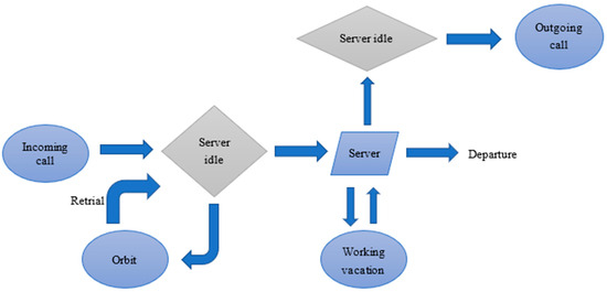
Figure 1. Two-way communication retrial queue with synchronous working vacation.

2.2. Markov Chain and Balance Equations

We denote the number of servers busy serving incoming and outgoing calls at time t by $n_1\left(t\right)$ and $n_2\left(t\right)$, respectively. Also, $C\left(t\right)$ and $M\left(t\right)$ are the server state and the number of customers in orbit at time t, respectively, where

$$C\left(t\right)=\left\{\begin{array}{c}0, \mathrm{all} \mathrm{servers} \mathrm{are} \mathrm{on} \mathrm{vacation} \mathrm{at} \mathrm{time} t,\\ 1, \mathrm{no} \mathrm{servers} \mathrm{are} \mathrm{on} \mathrm{vacation} \mathrm{at} \mathrm{time} t.\end{array}\right.$$

Thus, the process $\left\{\left(n_1\left(t\right),n_2\left(t\right),\mathrm{C}\left(t\right),\mathrm{M}\left(t\right)\right);t\ge 0\right\}$ is a continuous time Markov chain on the state space $\mathsf{\Omega }=\left\{\left(i,j,k,n\right):0\le i\le s,j=0,k=0,n\ge 0\right\}\cup \left\{\left(i,j,k,n\right):0\le i+j\le s,k=1,n\ge 0\right\}$.

Let ${\pi }_{i,j,k}\left(n\right)=\underset{t\to \infty }{\lim }\mathrm{P}\left\{\left(n_1\left(t\right), n_2\left(t\right), \mathrm{C}\left(t\right), \mathrm{M}\left(t\right)\right)\right\}$ be the limiting probabilities for the steady-state distribution. The system of governing steady-state equations is framed as follows:

$$\left(\lambda +\theta \right){\pi }_{0,0,0}\left(0\right)={{\mu }_3{\pi }_{1,0,0}\left(0\right)+\mu }_1{\pi }_{1,0,1}\left(0\right)+{\mu }_2{\pi }_{0,1,1}\left(0\right),$$

(1)

$$\left(\lambda +s\alpha \right){\pi }_{0,0,1}\left(0\right)=\theta {\pi }_{0,0,0}\left(0\right),$$

(2)

$$\left(\lambda +\theta +\sigma \right){\pi }_{i,0,1}\left(n\right)={\mu }_3{\pi }_{1,0,0}\left(n\right), n\ge 1,$$

(3)

$$\left(\lambda +s\alpha +\sigma \right){\pi }_{i,0,1}\left(n\right)={\mu }_1{\pi }_{1,0,1}\left(n\right)+{\mu }_2{\pi }_{0,1,1}\left(n\right)+\theta {\pi }_{0,0,0}\left(n\right),n\ge 1,$$

(4)

$$\begin{gathered} \left(\lambda +i{\mu }_3+\theta +\left(1-{\delta }_{n,0}\right)\sigma \right){\pi }_{i,0,0}\left(n\right)=\lambda {\pi }_{i-1,0,0}\left(n\right)+\left(i+1\right){\mu }_3{\pi }_{i+1,0,0}\left(n\right)+ \\ \sigma {\pi }_{i-1,0,0}\left(n+1\right),1\le i\le s-1, n\ge 0, \end{gathered}$$

(5)

$$\begin{gathered} \left(\lambda +i{\mu }_1+\left(s-i\right)\alpha +\left(1-{\delta }_{n,0}\right)\sigma \right){\pi }_{i,0,1}\left(n\right)=\lambda {\pi }_{i-1,0,1}\left(n\right)+\left(i+ \\ 1\right){\mu }_1{\pi }_{i+1,0,1}\left(n\right)+{\mu }_2{\pi }_{i,1,1}\left(n\right)+\theta {\pi }_{i,0,0}\left(n\right)+\sigma {\pi }_{i-1,0,1}\left(n+1\right),1\le i\le s-1, n\ge 0, \end{gathered}$$

(6)

$$\begin{gathered} \left(\lambda +i{\mu }_1+j{\mu }_2+\left(s-i-j\right)\alpha +\left(1-{\delta }_{n,0}\right)\sigma \right){\pi }_{i,j,1}\left(n\right)=\left(s-i-j+ \\ 1\right)\alpha {\pi }_{i,j-1,1}\left(n\right)+\lambda {\pi }_{i-1,j,1}\left(n\right)+\left(i+1\right){\mu }_1{\pi }_{i+1,j,1}\left(n\right)+\left(j+1\right){\mu }_2{\pi }_{i,j+1,1}\left(n\right)+ \\ \sigma {\pi }_{i-1,j,1}\left(n+1\right),0\le i\le s-j-1, 1\le j\le s-1, n\ge 0, \end{gathered}$$

(7)

$$\begin{gathered} \left(b\lambda +s{\mu }_3+\theta \right){\pi }_{s,0,0}\left(n\right)=b\lambda {\pi }_{s,0,0}\left(n-1\right)+\lambda {\pi }_{s-1,0,1}\left(n\right)+\sigma {\pi }_{s-1,0,0}\left(n+1\right), \\ n\ge 0, \end{gathered}$$

(8)

$$\begin{gathered} \left(b\lambda +\left(s-j\right){\mu }_1+j{\mu }_2\right){\pi }_{s-j,j,1}\left(n\right)=b\lambda {\pi }_{s-j,j,1}\left(n-1\right)+\alpha {\pi }_{s-j,j-1,1}\left(n\right)+ \\ \lambda {\pi }_{s-j-1,j,1}\left(n\right)+\theta {\delta }_{j,0}{\pi }_{s-j,j,0}\left(n\right)+\sigma {\pi }_{s-j-1,j,1}\left(n+1\right), 0\le j\le s, n\ge 0. \end{gathered}$$

(9)

The normalizing condition is

$${\sum }_{n=0}^{\infty }{\sum }_{i=0}^s{\pi }_{i,0,0}\left(n\right)+{\sum }_{n=0}^{\infty }{\sum }_{i=0}^s{\sum }_{j=0}^{s-i}{\pi }_{i,j,1}\left(n\right)=1,$$

(10)

where ${\delta }_{n,0}$ represents Kronecker’s delta and ${\pi }_{i,j,k}\left(n\right)=0$ if $\left(i, j, k, n\right)\notin \mathsf{\Omega }$.

3. System Analysis

This section provides a system analysis. First, a quasi-birth-and-death process formulation is provided to identify all the components of the involved infinitesimal generator and block matrices. Next, the steady-state probabilities are derived in matrix form, and ergodic condition is exported.

3.1. Infinitesimal Generator and Matrices

According to the matrix geometric method, the infinitesimal generator of the continuous time Markov process $\left\{\left(n_1\left(t\right), n_2\left(t\right), \mathrm{C}\left(t\right), \mathrm{M}\left(t\right)\right);t\ge 0\right\}$} is written in the form of a block matrix Q as

$$\mathbf{Q}=\left[\begin{array}{cc}\begin{array}{cc}{\mathbf{G}}^0& {\mathbf{G}}^u\\ {\mathbf{G}}^l& \mathbf{G}\end{array}& \begin{array}{cc}& \\ {\mathbf{G}}^u& \end{array}\\ \begin{array}{cc}& \ddots \\ & \end{array}& \begin{array}{cc}\ddots & \ddots \\ \ddots & \ddots \end{array}\end{array}\right],$$

(11)

where G⁰, G^u, G^l, and G are square matrices of order (s + 1)(s + 4)/2.

For the concerned model, we can represent the block structures of these matrices as

$${\mathbf{G}}^u=\left[\begin{array}{cc}\begin{array}{cc}{\mathbf{G}}_0^u& \\ & {\mathbf{G}}_1^u\end{array}& \begin{array}{cc}& \\ & \end{array}\\ \begin{array}{cc}& \\ & \end{array}& \begin{array}{cc}\ddots & \\ & {\mathbf{G}}_s^u\end{array}\end{array}\right],$$

$${\mathbf{G}}^l=\left[\begin{array}{cc}\begin{array}{cc}{\mathbf{G}}_0^l& \\ & {\mathbf{G}}_1^l\end{array}& \begin{array}{cc}& \\ & \end{array}\\ \begin{array}{cc}& \\ & \end{array}& \begin{array}{cc}\ddots & \\ & {\mathbf{G}}_s^l\end{array}\end{array}\right],$$

$$\mathbf{G}=\left[\begin{array}{cc}\begin{array}{ccc}{\mathbf{B}}_0& {\mathbf{B}}_1& \\ & {\mathbf{A}}_0& {\mathbf{A}}_0^{+}\\ & {\mathbf{A}}_1^{-}& {\mathbf{A}}_1\end{array}& \begin{array}{ccc}& & \\ & & \\ {\mathbf{A}}_1^{+} & & \end{array}\\ \begin{array}{ccc}& & \ddots \\ & & \\ & & \end{array}& \begin{array}{ccc}\ddots & \ddots & \\ {\mathbf{A}}_{s-1}^{-}& {\mathbf{A}}_{s-1}& {\mathbf{A}}_{s-1}^{+}\\ & {\mathbf{A}}_s^{-}& {\mathbf{A}}_S\end{array}\end{array}\right],$$

where ${\mathbf{G}}_j^u \left(0\le j\le s\right)$, ${\mathbf{G}}_j^l \left(0\le j\le s\right)$, ${\mathbf{B}}_0$, ${\mathbf{B}}_1$, ${\mathbf{A}}_j \left(0\le j\le s\right)$, ${\mathbf{A}}_j^{+} \left(0\le j\le s-1\right)$, and ${\mathbf{A}}_j^{-} \left(1\le j\le s\right)$ are (s − j + 1) × (s − j + 1), (s − j + 1) × (s − j + 1), (s + 1) × (s + 1), (s + 1) × (s + 1), (s − j + 1) × (s − j + 1), (s − j + 1) × (s − j), and (s − j + 1) × (s − j + 2) matrices, respectively, with entries given by

$${\mathbf{G}}_j^u\left[k,k\prime \right]=\left\{\begin{array}{l}b\lambda , k^{\prime }=k=s-j+1,\\ 0, \mathrm{in} \mathrm{other} \mathrm{cases};\end{array}\right.$$

$${\mathbf{G}}_j^l\left[k,k\prime \right]=\left\{\begin{array}{l}\sigma , k^{\prime }=k+1, 1\le k\le s-j,\\ 0, \mathrm{in} \mathrm{other} \mathrm{cases}; \end{array}\right.$$

$${\mathbf{B}}_0\left[k,k^{\prime }\right]=\left\{\begin{array}{l}\lambda , k^{\prime }=k+1, 1\le k\le s, \\ \left(k-1\right){\mu }_3, k^{\prime }=k-1, 2\le k\le s+1, \\ -\left(\lambda +\left(k-1\right){\mu }_3+\theta +\sigma \right), k^{\prime }=k, 1\le k\le s,\\ -\left(b\lambda +s{\mu }_3+\theta \right), k^{\prime }=k=s+1, \\ 0, \mathrm{in} \mathrm{other} \mathrm{cases}; \end{array}\right.$$

$${\mathbf{B}}_1\left[k,k\prime \right]=\left\{\begin{array}{l}\theta , k^{\prime }=k, 1\le k\le s+1,\\ 0, \mathrm{in} \mathrm{other} \mathrm{cases}; \end{array}\right.$$

$${\mathbf{A}}_j^{+}\left[k,k\prime \right]=\left\{\begin{array}{l}\left(s-j+1-k\right)\alpha , k^{\prime }=k, 1\le k\le s-j,\\ 0, \mathrm{in} \mathrm{other} \mathrm{cases}; \end{array}\right.$$

$${\mathbf{A}}_j\left[k,k\prime \right]=\left\{\begin{array}{l} \lambda , k^{\prime }=k+1, 1\le k\le s-j, \\ k{\mu }_1, k^{\prime }=k-1, 2\le k\le s-j+1, \\ -\left(\lambda +\left(k-1\right){\mu }_1+j{\mu }_2+\left(s-j+1-k\right)\alpha +\sigma \right), k^{\prime }=k, 1\le k\le s,\\ -\left(b\lambda +\left(s-j\right){\mu }_1+j{\mu }_2\right), k^{\prime }=k=s+1, \\ 0, \mathrm{in} \mathrm{other} \mathrm{cases}; \end{array}\right.$$

$${\mathbf{A}}_j^{-}\left[k,k\prime \right]=\left\{\begin{array}{l}j{\mu }_2, k^{\prime }=k, 1\le k\le s-j+1,\\ 0, \mathrm{in} \mathrm{other} \mathrm{cases}. \end{array}\right.$$

The matrix ${\mathbf{G}}^0$ is the same as G, but the element of ${\mathbf{G}}^0\left[s+3, s+2\right]$ is shifted to the position of ${\mathbf{G}}^0\left[s+3, 1\right]$, the element of ${\mathbf{G}}^0\left[2s+3, s+2\right]$ is shifted to the position of ${\mathbf{G}}^0\left[2s+3,1\right]$, and the retrial rate σ is ignored.

3.2. Stationary Distribution

Assume that $\mathsf{\Pi }=\left[\begin{array}{ccc}\mathsf{\Pi }\left(0\right),& \mathsf{\Pi }\left(1\right),& \cdots \end{array}\right]$ represents the steady-state probability vector of Q. Also, $\mathsf{\Pi }\left(n\right)=\left[\begin{array}{cc}\begin{array}{ccc}{\pi }_{0,0,0}\left(n\right)& \cdots & {\pi }_{s,0,0}\left(n\right)\end{array}& \begin{array}{ccc}{\mathsf{\pi }}_0\left(n\right)& \cdots & {\mathsf{\pi }}_s\left(n\right)\end{array}\end{array}\right]$ and ${\mathsf{\pi }}_j\left(n\right)=\left[\begin{array}{ccc}{\pi }_{0,j,1}\left(n\right)& \cdots & {\pi }_{s-j,j,1}\left(n\right)\end{array}\right]$ for $0\le j\le s$.

We can rewrite Equations (1)–(10) in the matrix form as ΠQ = 0 and $\sum _{n=0}^{\infty }\mathsf{\Pi }\left(n\right)\mathbf{e}=1$, where 0 and e represent a row and a column vector with an appropriate size with all zero and all one entries, respectively.

Note that from Neuts [23], there is a matrix R, such that $\mathsf{\Pi }\left(n\right)=\mathsf{\Pi }\left(n-1\right)\mathbf{R}$. This implies that $\mathsf{\Pi }\left(n\right)=\mathsf{\Pi }\left(0\right){\mathbf{R}}^n$. Here, R is the minimal non-negative solution of

$${\mathbf{G}}^u+\mathbf{R}\mathbf{G}+{\mathbf{R}}^2{\mathbf{G}}^l=0,$$

(12)

with a spectral radius less than one. Since it is difficult for R to obtain the explicit expression by solving Equation (12), researchers could use different methods such as a successive substitution approach to evaluate R. In the numerical illustration, the following procedure will be implemented to approximate R.

We can define I as an identity matrix. The first equation of ΠQ = 0 can be written as the following by replacing $\mathsf{\Pi }\left(1\right)$ with $\mathsf{\Pi }\left(1\right)=\mathsf{\Pi }\left(0\right)\mathbf{R}$:

$$\mathsf{\Pi }\left(0\right){\mathbf{G}}^0+\mathsf{\Pi }\left(0\right)\mathbf{R}{\mathbf{G}}^l=0.$$

(13)

And $\sum _{n=0}^{\infty }\mathsf{\Pi }\left(n\right)\mathbf{e}=1$ can be re-written as

$${\sum }_{n=0}^{\infty }\mathsf{\Pi }\left(n\right)\mathbf{e}=\mathsf{\Pi }\left(0\right){\left(\mathbf{I}-\mathbf{R}\right)}^{-1}\mathbf{e}=1,$$

(14)

where I is an identity matrix. These two equations can be used to determine Π(0).

3.3. Ergodicity

Consider that the matrix $\mathbf{H}={\mathbf{G}}^u+\mathbf{G}+{\mathbf{G}}^l$=. Let $\mathbf{p}=\left[\begin{array}{cc}\begin{array}{cc}{\mathbf{p}}_{0,0}& {\mathbf{p}}_{0,1}\end{array}& \begin{array}{cc}\cdots & {\mathbf{p}}_{s,1}\end{array}\end{array}\right]$ is the invariant probability vector of H, where ${\mathbf{p}}_{0,0}=\left[\begin{array}{cc}\begin{array}{cc}{p}_{0,0,0}& p_{1,0,0}\end{array}& \begin{array}{cc}\cdots & p_{s,0,0}\end{array}\end{array}\right]$ and ${\mathbf{p}}_{j,1}=\left[\begin{array}{cc}\begin{array}{ll}{p}_{0,j,1}& p_{1,j,1}\end{array}& \begin{array}{ll}\cdots & p_{s-j,j,1}\end{array}\end{array}\right]$ 0 ≤ j ≤ s. Therefore, p satisfies the following criteria: pH = 0 and pe = 1. The condition for the ergodicity of the Markov chain $\left\{\left(n_1\left(t\right),n_2\left(t\right),\mathrm{C}\left(t\right)\right);t\ge 0\right\}$ is $\mathbf{p}{\mathbf{G}}^u\mathbf{e}<\mathbf{p}{\mathbf{G}}^l\mathbf{e}$. The ergodicity condition can be transformed to

$$\left(b\lambda +\sigma \right)P_B^{loss}<\sigma ,$$

(15)

where $P_B^{loss}=\sum _{j=0}^s{p}_{s-j,j,1}$ denotes the blocking probability of the corresponding loss system.

The ergodicity condition proposed by $\mathbf{p}{\mathbf{G}}^u\mathbf{e}<\mathbf{p}{\mathbf{G}}^l\mathbf{e}$ itself is unambiguous because the number of states for $\left\{\left(n_1\left(t\right), n_2\left(t\right), \mathrm{C}\left(t\right)\right);t\ge 0\right\}$ is finite. However, it does not seem to be easy to obtain a simple scalar form in terms of the given parameters. Below, a simple explicitness is obtained from (15) for the special case of s = 1. For the matrices, we have

$${\mathbf{G}}^u=\left[\begin{array}{cc}\begin{array}{ccc}0& 0& 0\\ 0& b\lambda & 0\\ 0& 0& 0\end{array}& \begin{array}{cc}0& 0\\ 0& 0\\ 0& 0\end{array}\\ \begin{array}{ccc}0& 0& 0\\ 0& 0& 0\end{array}& \begin{array}{cc}b\lambda & 0\\ 0& b\lambda \end{array}\end{array}\right],$$

$${\mathbf{G}}^l=\left[\begin{array}{cc}\begin{array}{ccc}0& \sigma & 0\\ 0& 0& 0\\ 0& 0& 0\end{array}& \begin{array}{cc}0& 0\\ 0& 0\\ \sigma & 0\end{array}\\ \begin{array}{ccc}0& 0& 0\\ 0& 0& 0\end{array}& \begin{array}{cc}0& 0\\ 0& 0\end{array}\end{array}\right],$$

$$\mathbf{G}=\left[\begin{array}{ccc}\begin{array}{cc}-\left(\lambda +\theta +\sigma \right)& \lambda \\ {\mu }_3& -\left(b\lambda +{\mu }_3+\theta \right)\end{array}& \begin{array}{cc}\theta & 0\\ 0 & \theta \end{array}& \begin{array}{c}0\\ 0\end{array}\\ \begin{array}{cc}0 & 0\\ 0 & 0\end{array}& \begin{array}{cc}-\left(\lambda +\alpha +\sigma \right)& \lambda \\ {\mu }_1& -\left(b\lambda +{\mu }_1\right)\end{array}& \begin{array}{c}\alpha \\ 0\end{array}\\ \begin{array}{cc}0 & 0\end{array}& \begin{array}{cc}{\mu }_2 & 0\end{array}& -\left(b\lambda +{\mu }_2\right)\end{array}\right],$$

$$\mathbf{H}=\left[\begin{array}{ccccc}-\left(\lambda +\theta +\sigma \right)& \lambda +\sigma & \theta & 0& 0\\ {\mu }_3& -\left({\mu }_3+\theta \right)& 0& \theta & 0\\ 0& 0& -\left(\lambda +\alpha +\sigma \right)& \lambda +\sigma & \alpha \\ 0& 0& {\mu }_1& -{\mu }_1& 0\\ 0& 0& {\mu }_2& 0& -{\mu }_2\end{array}\right].$$

We have $p_{0,0,0}=0$, $p_{1,0,0}=0$, $p_{0,1,1}=\left(\mathit{\lambda }+\mathit{\sigma }\right)p_{0,0,1}/{\mathit{\mu }}_1$, and $p_{1,0,1}=\alpha p_{0,0,1}/{\mathit{\mu }}_2$. Hence, the ergodicity condition is

$$b\lambda \left(\frac{\mathit{\lambda }+\mathit{\sigma }}{{\mathit{\mu }}_1}+\frac{\mathit{\alpha }}{{\mathit{\mu }}_2}\right)<\sigma .$$

If we set b = 1, then the ergodicity condition is consistent with Equation (15) in Phung-Duc and Rogiest [24].

4. System Characteristics and Cost Function

We compute system characteristics and average operating cost in terms of the steady-state probabilities in this section.

4.1. System Characteristics

If the system is in stability condition, we can obtain the expressions of the system characteristics listed below.

The average number of calls in orbit (average orbit length) is

$$E\left[N\right]={\sum }_{n=0}^{\infty }n\left({\sum }_{i=0}^s{\pi }_{i,0,0}\left(n\right)\right)+{\sum }_{n=0}^{\infty }n\left({\sum }_{j=0}^s{\sum }_{i=0}^{s-j}{\pi }_{i,j,1}\left(n\right)\right).$$

By Little’s Law, the average waiting time of a call in orbit is

$$E\left[W\right]=\frac{E\left[N\right]}{b\lambda }=\frac{1}{b\lambda }{\sum }_{n=0}^{\infty }n\left({\sum }_{i=0}^s{\pi }_{i,0,0}\left(n\right)\right)+{\sum }_{n=0}^{\infty }n\left({\sum }_{j=0}^s{\sum }_{i=0}^{s-j}{\pi }_{i,j,1}\left(n\right)\right).$$

The average number of incoming calls during the vacation period is

$$E\left[S_0\right]={\sum }_{n=0}^{\infty }{\sum }_{i=0}^{s}i\times {\pi }_{i,0,0}\left(n\right).$$

The average number of incoming calls during the non-vacation period is

$$E\left[S_1\right]={\sum }_{n=0}^{\infty }{\sum }_{j=0}^s{\sum }_{i=0}^{s-j}i\times {\pi }_{i,j,1}\left(n\right).$$

The average number of outgoing calls during the non-vacation period is

$$E\left[S_2\right]={\sum }_{n=0}^{\infty }{\sum }_{j=0}^{s}j{\sum }_{i=0}^{s-j}{\pi }_{i,j,1}\left(n\right).$$

The average number of servers being busy during the non-vacation period is defined as

$$E\left[B\right]={\sum }_{n=0}^{\infty }{\sum }_{j=0}^s{\sum }_{i=0}^{s-j}\left(i+j\right){\pi }_{i,j,1}\left(n\right)=E\left[S_1\right]+E\left[S_2\right].$$

The average number of servers on vacation, whether busy or not, is calculated as

$$E\left[V\right]={\sum }_{n=0}^{\infty }s\left({\sum }_{i=0}^s{\pi }_{i,0,0}\left(n\right)\right).$$

The average number of idle servers is calculated as

$$E\left[I\right]=s-E\left[B\right]-E\left[V\right].$$

The server utilization at the steady state is

$$U=\frac{E\left[S_0\right]+E\left[S_1\right]+E\left[S_2\right]}{s}.$$

4.2. Cost Function

Assume that the structure of the average operating cost is linear cost structure based on the cost elements associated with different system characteristics. First, define the cost elements involved in the average operating cost as follows:

r₁ ≡ the cost of a retrial customer;

r₂ ≡ the cost of an idle server during the non-vacation period;

r₃ ≡ the cost of a busy server during the non-vacation period;

r₄ ≡ the cost of a vacation server;

r₅ ≡ the cost of providing a vacation.

Then, the average operating cost is

$$OC=r_{1}E\left[N\right]+r_{2}E\left[I\right]+r_{3}E\left[B\right]+r_{4}E\left[V\right]+r_5\theta .$$

5. Numerical Illustration

If the ergodicity condition is satisfied, this section presents some numerical results on the system characteristics and optimization results. We perform sensitivity analysis to illustrate the effect of system descriptors on the system characteristics.

5.1. Sensitivity Analysis

For the sensitivity analysis, the default parameters are fixed as s = 5, λ = 4, α = 3, μ₁ = 1.5, μ₂ = 1.5, μ₃ = 0.8, σ = 10, θ = 0.3, and b = 0.8, unless their values are mentioned in tables and figures.

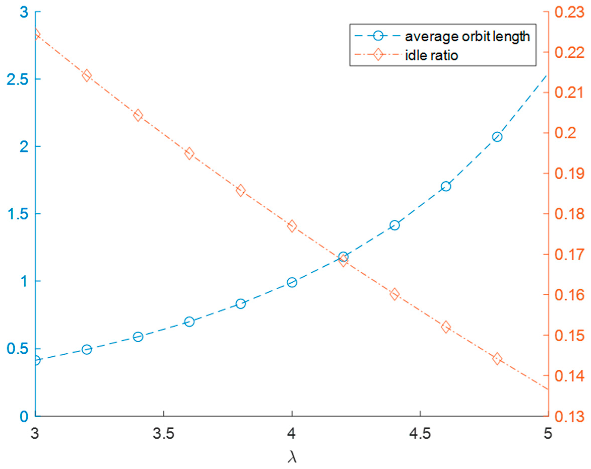
Table 1 and Figure 2 clearly show that the average orbit length increases whenever the incoming call rate increases. At the same time, the server idle time is reduced, and the average number of vacation servers decreases.

Table 1. Effect of incoming call rate.

λ	E[N]	1-U	E[B]	E[V]
3	0.224	0.224	3.720	0.308
3.2	0.494	0.214	3.777	0.283
3.4	0.588	0.204	3.832	0.259
3.6	0.700	0.195	3.887	0.236
3.8	0.833	0.186	3.940	0.214
4	0.991	0.177	3.993	0.193
4.2	1.182	0.168	4.045	0.173
4.4	1.415	0.160	4.097	0.153
4.6	1.704	0.152	4.147	0.135
4.8	2.070	0.144	4.197	0.117
5	2.546	0.136	4.246	0.100

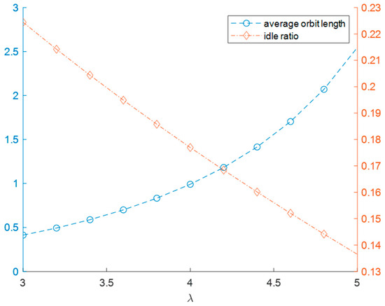
Figure 2. Average orbit length and idle ratio vs. λ.

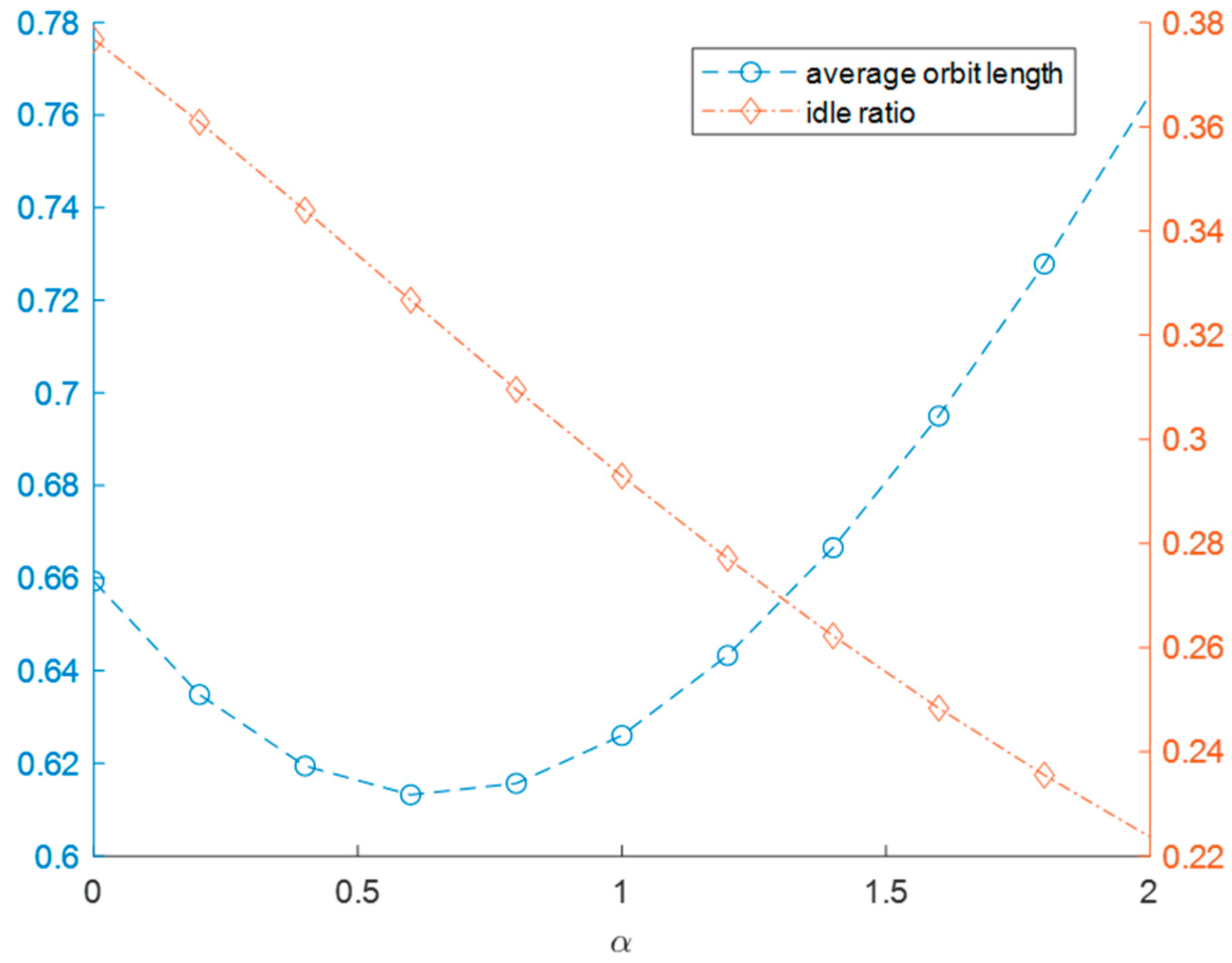
Table 2 and Figure 3 demonstrate that the increasing nature of the average orbit length first decreases and then increases as the outgoing call rate increases. For the larger outgoing call rate, if the server makes outgoing calls more frequently, it will have fewer opportunities to service incoming calls, resulting in a longer orbit length. On the other hand, the smaller the outgoing call rate, the longer the server takes to make outgoing calls, which results in the fact that the longer the server is idle, the more incoming calls it can serve. This threshold is related to the arrival rate of incoming calls. And the average number of vacation servers decreases. Simultaneously, the server idle time is reduced. Table 3 and Figure 4 display that the server idle time decreases slightly whenever the retrial rate increases. At the same time, the average number of vacation servers increases, and the average orbit length of incoming calls decreases.

Table 2. Effect of outgoing call rate.

α	E[N]	1-U	E[B]	E[V]
0	0.659	0.377	1.886	1.947
0.2	0.635	0.361	2.126	1.691
0.4	0.619	0.344	2.359	1.458
0.6	0.613	0.327	2.577	1.249
0.8	0.616	0.310	2.779	1.065
1	0.626	0.293	2.962	0.907
1.2	0.643	0.277	3.127	0.771
1.4	0.667	0.262	3.274	0.656
1.6	0.695	0.248	3.405	0.559
1.8	0.728	0.236	3.521	0.477
2	0.764	0.224	3.624	0.407

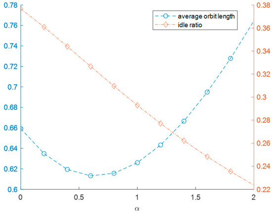
Figure 3. Average orbit length and idle ratio vs. α.

Table 3. Effect of retrial rate.

σ	E[N]	1-U	E[B]	E[V]
3	8.602	0.173	4.107	0.049
4	3.314	0.174	4.065	0.102
5	2.170	0.175	4.041	0.134
6	1.669	0.176	4.025	0.154
7	1.389	0.176	4.013	0.168
8	1.209	0.177	4.005	0.179
9	1.083	0.177	3.998	0.187
10	0.991	0.177	3.993	0.193

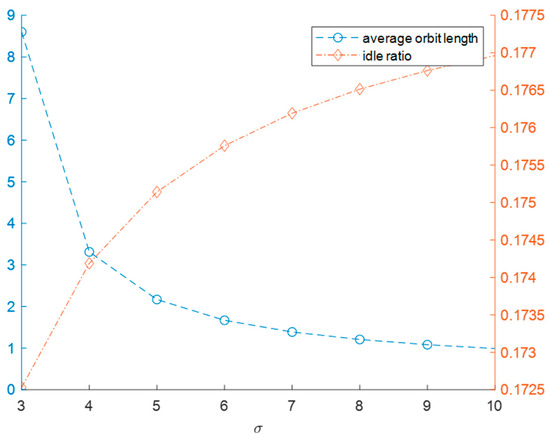
Figure 4. Average orbit length and idle ratio vs. σ.

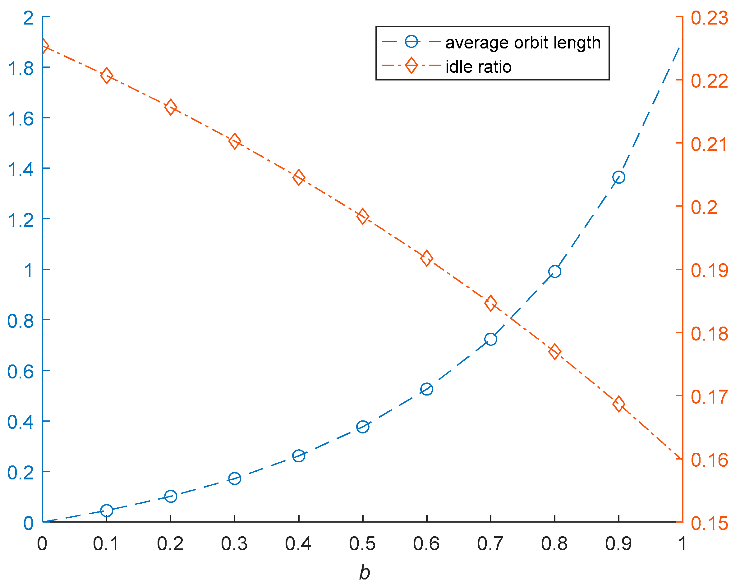
Table 4 and Figure 5 clearly show that the non-balking rate has an increasing trend for the average orbit length, while the non-balking rate has an increasing tendency for the server idle time and the average number of vacation servers. This is reasonable since when the non-balking rate is increasing, this means that there are more incoming calls joining the orbit.

Table 4. Effect of non-balking rate.

b	E[N]	1-U	E[B]	E[V]
0.0	0.000	0.225	3.697	0.302
0.1	0.045	0.221	3.725	0.292
0.2	0.101	0.216	3.755	0.281
0.3	0.172	0.210	3.787	0.270
0.4	0.262	0.205	3.822	0.257
0.5	0.376	0.198	3.860	0.243
0.6	0.526	0.192	3.900	0.228
0.7	0.723	0.185	3.945	0.211
0.8	0.991	0.177	3.993	0.193
0.9	1.365	0.169	4.046	0.173
1.0	1.908	0.160	4.104	0.151

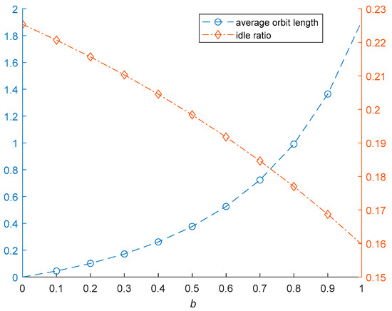
Figure 5. Average orbit length and idle ratio vs. b.

5.2. Optimization

The aim of optimization is to determine the optimal outgoing calls rate and optimal vacation rate. Except for operating cost consideration, average orbit length and server utilization are also important system characteristics in the modeling of any queue. Therefore, we will design a tri-objective optimization problem as follows:

Minimize:	y1(α, θ) = OC
Minimize:	y2(α, θ) = 1-U
Minimize:	y3(α, θ) = E[W]
Subject to:	$\mathbf{p}{\mathbf{G}}^u\mathbf{e}<\mathbf{p}{\mathbf{G}}^l\mathbf{e}$,
	α > 0,
	θ > 0.

As can be seen from the expressions of the average operating cost and loss function, the analytical solution is difficult to derive. Computational software is applied to solve the optimization problem numerically. Here, the computer software MATLAB R2022a is used to implement a multi-objective genetic algorithm to solve the above tri-objective optimization problem. Readers can refer to Konak et al. [25] for a detailed overall flow of the general multi-objective genetic algorithm. The multi-objective genetic algorithm pseudocode is shown below (Algorithm 1).

Algorithm 1. Multi-Objective Genetic Algorithm

Begin Initialize population Evaluate fitness of each individual in the population While not termination criteria do Select the best individuals to reproduce Apply crossover and mutation operations Evaluate population Update population End While Output the best solution End

The optimization analysis has been performed for the default parameters, fixed as follows:

s = 5, λ = 4, μ₁ = 1.5, μ₂ = 1.5, μ₃ = 0.8, σ = 10, b = 0.8, r₁ = 20, r₂ = 25, r₃ = 100, r₄ = 50, r₅ = 5.

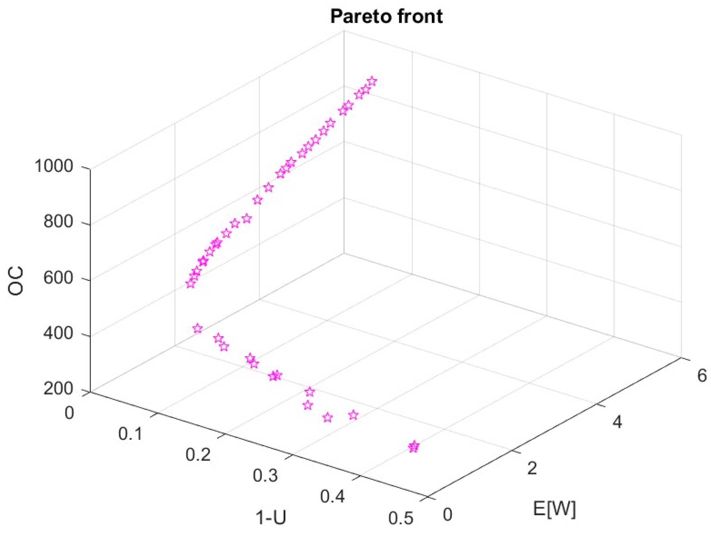
Figure 6 reveals that the higher the average operating cost, the lower the expected loss is. Table 5 presents the Pareto optimal solution sets. At this time, the operation manager needs to decide which set of solutions to implement. There is no right or wrong choice; it depends on the decision maker’s own experience and judgment. To help the decision maker make decisions based on the Pareto optimal solution sets, Solution #3 and Solution #4 are selected from Table 5 as reference schemes. Solution #3 is the solution that achieves the minimum average waiting time in orbit. This is a good solution if the decision maker cares about service quality. Solution #4 is chosen based on the assigned weight of these three objectives (0.5, 0.2, 0.3). The steps are as follows:

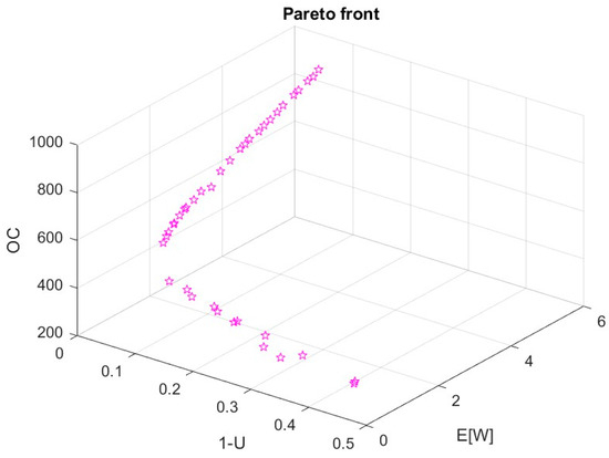
Figure 6. Pareto front solutions found by multi-objective genetic algorithm.

Table 5. Optimal solutions for the multi-objective optimization model.

#	α*	θ*	y2(α*, θ*)	y3(α*, θ*)	y1(α*, θ*)	#	α*	θ*	y2(α*, θ*)	y3(α*, θ*)	y1(α*, θ*)
1	0.0029	0.1719	0.3303	0.3469	328.0764	21	1.8214	6.1886	0.2302	0.2028	458.0735
2	11.9983	9.3615	0.0607	5.6859	887.9584	22	11.9658	7.9205	0.0608	5.5383	871.2552
3	0.0037	6.9089	0.4770	0.0577	362.5594	23	10.4485	7.6545	0.0682	2.3350	662.1581
4	0.0225	0.1094	0.2909	0.5078	329.4854	24	11.2708	8.7965	0.0639	3.4762	742.4771
5	11.6941	8.1659	0.0620	4.5257	807.2304	25	0.0034	4.6110	0.4753	0.0581	352.2698
6	9.1094	8.1264	0.0764	1.4475	604.6404	26	0.8523	7.8445	0.3177	0.1256	429.1866
7	9.8066	8.6442	0.0718	1.8235	632.9824	27	11.3963	9.2969	0.0634	3.7387	762.0079
8	1.3339	7.3381	0.2670	0.1639	447.7312	28	11.6304	7.6043	0.0623	4.3340	792.0429
9	8.3530	7.7555	0.0819	1.1600	582.2932	29	2.7920	5.0038	0.1808	0.2834	475.5974
10	1.4171	5.0161	0.2608	0.1703	438.9278	30	9.1510	8.3405	0.0761	1.4663	607.0263
11	3.0315	8.2727	0.1712	0.3045	496.8050	31	4.5492	1.8434	0.1310	0.4534	489.1407
12	11.9288	8.7767	0.0610	5.3783	865.2380	32	10.2003	7.3972	0.0695	2.1116	646.0564
13	11.5663	8.1376	0.0626	4.1553	783.1670	33	11.3412	8.5499	0.0636	3.6194	750.5374
14	10.9316	7.1698	0.0656	2.9075	697.3245	34	11.1095	7.7431	0.0647	3.1834	718.1778
15	0.0225	0.1094	0.2909	0.5078	329.4854	35	11.7452	8.9743	0.0618	4.6904	821.8985
16	0.4143	7.1925	0.3845	0.0905	399.4445	36	11.8315	8.6844	0.0614	4.9937	839.9988
17	1.9076	8.6592	0.2241	0.2100	473.0613	37	11.8663	8.8001	0.0612	5.1255	849.0706
18	10.7258	1.9636	0.0667	2.6367	653.5573	38	11.5096	7.4507	0.0628	4.0075	770.1729
19	7.7684	8.3220	0.0869	0.9913	572.4912	39	9.8691	8.6911	0.0715	1.8647	635.9991
20	0.0029	0.1719	0.3303	0.3469	328.0764	40	8.6137	8.1724	0.0799	1.2486	590.8052

-

Step 1: Normalize the three objective values for each solution.

-

Step 2: Multiply their respective weights and add these three values.

-

Step 3: Sort the values obtained in step 2, and the first solution is the optimal solution.

6. Conclusions

This work investigated a synchronous working vacation model of a retrial queue, in which there are two types of arrivals, incoming calls made by customers and outgoing calls made by idle servers. The servers have no information about how many calls exist in orbit. So even with many calls in orbit, outgoing call activity is still possible. We utilized the matrix geometric technique to derive the stationary probabilities, ergodic condition, and system characteristics. At last, we implemented numerical examples to observe the trends of system characteristics for different parametric values and proposed a related optimization issue. The sensitivity analysis in this study can provide useful insights to decision makers to improve service quality. Through numerical examples, it is found that the server idle time is reduced with an increase in the incoming/outgoing call rate and retrial rate. The orbit length is found to decrease with an increase in the incoming/outgoing call rate and retrial rate. The average number of vacation servers decreases with an increase in the incoming call rate and outgoing call rate. The graph behavior was found to be consistent with theoretical expectations. Via a multi-objective genetic algorithm, the entire set of Pareto optimal solutions is determined. We also provide some reference solutions to illustrate how the decision maker can make decisions based on the Pareto optimal solution set.

One limitation of this paper is to assume that all the involved random variables in the model introductions are exponentially distributed. Extending our analysis to consider the general distribution is a future research direction. Additionally, similar models incorporating practical concepts such as working breakdown, batch arrival, immediate feedback, optional type service, negative customers, priority service, and many others can be studied.

References

- Kim, J.; Kim, B. A survey of retrial queueing systems. Ann. Oper. Res. 2016, 247, 3–36. [Google Scholar] [CrossRef]
- Phung-Duc, T. Retrial Queueing Models: A Survey on Theory and Applications. arXiv 2019, arXiv:1906.09560. [Google Scholar]
- Ke, J.C.; Chang, F.M.; Liu, T.H. M/M/c balking retrial queue with vacation. Qual. Technol. Quant. Manag. 2019, 16, 54–66. [Google Scholar] [CrossRef]
- Zhang, Y. Strategic behavior in the constant retrial queue with a single vacation. RAIRO Oper. Res. 2020, 54, 569–583. [Google Scholar] [CrossRef]
- Liu, T.H.; Chang, F.M.; Ke, J.C.; Sheu, S.H. Optimization of retrial queue with unreliable servers subject to imperfect coverage and reboot delay. Qual. Technol. Quant. Manag. 2022, 19, 428–453. [Google Scholar] [CrossRef]
- Govindan, A.; Jayaraj, U. Analysis of mixed priority retrial queueing system with two way communication and working breakdown. J. Math. Model. 2018, 6, 195–212. [Google Scholar]
- Nazarov, A.; Phung-Duc, T.; Paul, S. Slow retrial asymptotics for a single server queue with two-way communication and Markov modulated Poisson Input. J. Syst. Sci. Syst. Eng. 2019, 28, 181–193. [Google Scholar] [CrossRef]
- Ayyappan, G.; Udayageetha, J.; Somasundaram, B. Analysis of non-pre-emptive priority retrial queueing system with two-way communication, Bernoulli vacation, collisions, working breakdown, immediate feedback and reneging. Int. J. Math. Oper. Res. 2020, 16, 480–498. [Google Scholar] [CrossRef]
- Kumar, M.S.; Dadlani, A.; Kim, K. Performance analysis of an unreliable M/G/1 retrial queue with two-way communication. Oper. Res. 2020, 20, 2267–2280. [Google Scholar]
- Ayyappan, G.; Gowthami, R. Analysis of MAP, PH2OA/PH1I, PH2O/1 retrial queue with vacation, feedback, two-way communication and impatient customers. Soft Comput. 2021, 25, 9811–9838. [Google Scholar] [CrossRef]
- Lee, S.W.; Kim, B.; Kim, J. Analysis of the waiting time distribution in M/G/1 retrial queues with two way communication. Ann. Oper. Res. 2022, 310, 505–518. [Google Scholar] [CrossRef]
- Sztrik, J.; Tóth, Á.; Pintér, Á. The Effect of Operation Time of the Server on the Performance of Finite-Source Retrial Queues with Two-Way Communications to the Orbit. J. Math. Sci. 2022, 267, 196–204. [Google Scholar] [CrossRef]
- Tóth, Á.; Sztrik, J. Analysis of retrial queueing systems with two-way communication and impatient customers using simulation. Ann. Math. Et Inform. 2023, 58, 160–169. [Google Scholar] [CrossRef]
- Yang, D.Y.; Wu, C.H. Performance analysis and optimization of a retrial queue with working vacations and starting failures. Math. Comput. Model. Dyn. Syst. 2019, 25, 463–481. [Google Scholar] [CrossRef]
- Li, T.; Zhang, L.; Gao, S. An M/G/1 retrial queue with balking customers and Bernoulli working vacation interruption. Qual. Technol. Quant. Manag. 2019, 16, 511–530. [Google Scholar] [CrossRef]
- Li, T.; Zhang, L.; Gao, S. An M/G/1 retrial queue with single working vacation under Bernoulli schedule. RAIRO-Oper. Res. 2020, 54, 471–488. [Google Scholar] [CrossRef]
- Gupta, P.; Kumar, N. Performance analysis of retrial queueing Model with working vacation, interruption, waiting server, breakdown and repair. Int. J. Sci. Res. 2021, 13, 833–844. [Google Scholar] [CrossRef]
- Muthusamy, S.; Devadoss, N.; Ammar, S.I. Reliability and optimization measures of retrial queue with different classes of customers under a working vacation schedule. Discret. Dyn. Nat. Soc. 2022, 2022, 6806104. [Google Scholar] [CrossRef]
- Pazhani, S.; Murugan, B.; Keerthana, R. An M/G/1 feedback retrial queue with working vacation and a waiting server. J. Comput. 2023, 31, 61–79. [Google Scholar]
- Shanmugam, B.; Saravanarajan, M.C. Unreliable retrial queueing system with working vacation. AIMS Math. 2023, 8, 24196–24224. [Google Scholar] [CrossRef]
- Chen, Z.; Xu, H.; Huo, H. Optimal queuing strategies for an M/G/1 retrial queue system with RWV and ISEV policies. ANZIAM J. 2024, 1–27. [Google Scholar] [CrossRef]
- Sundararaman, M.; Narasimhan, D.; Rajadurai, P. Performance Analysis of Two Different Types of Waiting Queues with Working Vacations. J. Math. 2024, 2024, 5829171. [Google Scholar] [CrossRef]
- Neut, M.F. Matrix-Geometric Solutions in Stochastic Models. Master’s Thesis, John Hopkins University, Baltimore, MD, USA, 1981. [Google Scholar]
- Phung-Duc, T.; Rogiest, W. Two Way Communication Retrial Queues with Balanced Call Blending. In Proceedings of the Analytical and Stochastic Modeling Techniques and Applications. ASMTA 2012, Grenoble, France, 4–6 June 2012. [Google Scholar]
- Konak, A.; Coit, D.W.; Smith, A.E. Multi-objective optimization using genetic algorithms: A tutorial. Reliab. Eng. Syst. Saf. 2006, 91, 992–1007. [Google Scholar] [CrossRef]
Disclaimer/Publisher’s Note: The statements, opinions and data contained in all publications are solely those of the individual author(s) and contributor(s) and not of MDPI and/or the editor(s). MDPI and/or the editor(s) disclaim responsibility for any injury to people or property resulting from any ideas, methods, instructions or products referred to in the content. |
© 2024 by the authors. Licensee MDPI, Basel, Switzerland. This article is an open access article distributed under the terms and conditions of the Creative Commons Attribution (CC BY) license (https://creativecommons.org/licenses/by/4.0/).