A Higher-Order Extended Cubature Kalman Filter Method Using the Statistical Characteristics of the Rounding Error of the System Model

Abstract

The cubature Kalman filter (CKF) cannot accurately estimate the nonlinear model, and these errors will have an impact on the accuracy. In order to improve the filtering performance of the CKF, this paper proposes a new CKF method to improve the estimation accuracy by using the statistical characteristics of rounding error, establishes a higher-order extended cubature Kalman filter (RHCKF) for joint estimation of sigma sampling points and random variables of rounding error, and gives a solution method considering the rounding error of multi-level approximation of the original function in the undermeasured dimension. Finally, numerical simulations show that the RHCKF has a better estimation effect than the CKF, and that the filtering accuracy is improved by using the information of the higher-order rounding error, which also proves the effectiveness of the method.

1. Introduction

Nonlinear state estimation is a popular research field, which is widely used in chemical processes, target tracking, signal processing, macroeconomic forecasting, and other engineering fields [1,2]. Nonlinear filtering is an important method to solve the nonlinear state estimation, and there are many research results. Ito et al. proposed a Gaussian nonlinear filtering framework and gave the optimal solution of nonlinear filtering under the Gaussian assumption [3]. Arellano-Valle et al. (2018) proposed the Kalman filter based on the skew-normal distribution as a non-Gaussian assumption of innovations [4]. It is difficult to get the optimal solution in practical processing; thus, only suboptimal approximation methods can be used instead. The commonly used nonlinear filtering algorithms include the extended Kalman filter (EKF) [5], untraceable Kalman filter (UKF) [6], and cubature Kalman filter (CKF) [7]. Among them, the EKF transforms the nonlinear state and the measurement function into a linear problem through the first-order Taylor series expansion [8]; the UKF overcomes the disadvantage of the EKF that the nonlinear function must be continuously differentiable and needs to solve the Jacobi matrix, it approximates the probability density function of the state by using a set of weighted sums of sampling points passed through a nonlinear function, and its filtering effect is significantly improved compared with that of the EKF [9]; however, when the dimensionality is too high, the UKF can be used to filter the state of the nonlinear state, which is a very important factor to improve the filtering effect. When the dimensionality is too high, the UKF filters poorly and even diverges, and its filtering effect is easily affected by the parameter settings [10,11]. Similar to the UKF, the CKF approximates a specific class of nonlinear integrals by obtaining a deterministic set of samples and weights through the spherical–radial Cubature law and moment matching [12]. The CKF has been widely studied and applied due to its advantages of high accuracy, low complexity, and good convergence. Compared with the EKF, the CKF does not need to calculate the Jacobi matrix and can eliminate the linearization error, which solves the theoretical limitations of the EKF; and compared with the UKF, the CKF has more stable performance and higher filtering accuracy when solving the filtering problem of high-dimensional strong nonlinear systems [13,14,15]. Thus, it has been widely used since proposed and has attracted many scholars who have attempted to improve it. Jia et al. [16] utilized the arbitrary-order fully symmetric spherical interpolation criterion and the moment matching method [17,18] to derive a higher-order spherical-phase-diameter cubature rule that can obtain arbitrary-order estimation accuracy. Using this rule, the high-order cubature Kalman filter (HCKF) [19] can be obtained, which improves the filtering accuracy of the CKF. In order to further improve the filtering accuracy, this paper proposes the high-order extended cubature Kalman filter considering rounding error, on the traditional CKF algorithm. This paper considers the rounding error that exists in the nonlinear approximation of the CKF. The algorithmic steps of the rounding error from the first to the general order are derived in detail, and it is proven by the simulation results that the new method improves the filtering accuracy.

The main contributions of this paper as follows: (1) proposing a new CKF method to improve the estimation accuracy by using the statistical characteristics of rounding error; and (2) adopting the idea of multi-level gradual approximation; the rounding error of the multi-level approximation of the original function in the undermeasured dimension is solved.

2. Problem Statement

Consider the following discrete-time nonlinear dynamic system:

$$\begin{array}{l}x(k+1)=f(x(k),k)+w(k)\\ y(k+1)=h(x(k+1),k+1)+v(k+1)\end{array}$$

(1)

where $k$ is the discrete time; $x(k)\in R^n$ is the state vector; $y(k+1)\in R^m$ is the observation vector; $f(\cdot )$ is the state transfer function; $h(\cdot )$ is the measurement function. System modeling errors $w(k)$ and $v(k+1)$ are uncorrelated white noise sequences.

The system satisfies the following assumptions:

$$E\left\{w(k)\right\}=0,E\left\{v(k)\right\}=0$$

$$E\left\{w(k)w^T(j)\right\}=Q(k){\delta }_{kj}$$

$$E\left\{v(k+1)v^T(j)\right\}=R(k+1){\delta }_{\{k+1,j\}}$$

where $Q(k)$ is the variance of noise $w(k)$; $R(k+1)$ is the variance of noise $v(k+1)$; ${\delta }_{kj}$ is the Kronecker product.

The cubature Kalman filtering algorithm converts nonlinear filtering into an integral problem of solving the product of a nonlinear function and a Gaussian probability density, and then approximates the state a posteriori probability density using a weighted sum of $2n$ cubature points. For an arbitrary distribution function $\rho (x)$, the integral problem is solved using the cubature integration criterion [20], the basic cubature points, and the corresponding weights obtained using the cubature criterion, as follows:

$${\displaystyle {\int }_{R^n}\rho (x)N(x;\mu ,\sum )dx\approx }{\displaystyle \sum _{i=1}^{2n}{\omega }_i\rho (\mu +\sqrt{\sum }}{\zeta }_i)$$

(2)

$${\zeta }_i=\sqrt{n}{e}_i, {\omega }_i=\frac{1}{2n}, i=1,2\cdots ,2n$$

(3)

where $N(x;\mu ,\sum )$ denotes that the state variable $x$ satisfying the mean $\mu$ is a Gaussian distribution with variance–covariance matrix $\sum$; ${\zeta }_i$ represents the product points; ${\omega }_i$ represents the corresponding weights, $\sum$ is the covariance and satisfies $\sum =\sqrt{\sum }{\sqrt{\sum }}^T$, ${\sqrt{\sum }}^T$ denotes the transpose of $\sqrt{\sum }$; $2n$ is the number of all cubature points, $n$ is the state dimension of the system; $e_i$ denotes the i-th cubature point. When $n=2$, the corresponding set of Cubature points is $e=\left[\begin{array}{cccc}1& 0& -1& 0\\ 0& 1& 0& -1\end{array}\right]$.

Assuming that the state estimates and covariances at the time of $k+1$ are $\widehat{x}(k+1|k+1)$ and $P(k+1|k+1)$, respectively, and the posterior probability density function at this time is $P(x(k+1))=N(\widehat{x}(k+1|k+1),P(k+1|k+1))$, the standard CKF algorithm was originally proposed in [21], and can be divided into temporal updating and measurement updating as follows.

• Time Update

(1) Initialize the state quantities and estimate the error covariance

$$\widehat{x}(0|0)=E\{x(0)\}$$

(4)

$$P(0|0)=E\{[x(0)-\widehat{x}(0|0)]{[x(0)-\widehat{x}(0|0)]}^T\}$$

(5)

(2) Construct a sigma point set under the nonlinear transformation $f(\cdot )$ to construct the point set ${\{x_i(k)\}}_{\mathrm{i}=1}^{2n}$, which contains a total of $2n$ points, where $x_i(k)$ are the sampling points obtained by sampling.

(3) Perform the Cholesky decomposition on $P(k|k)$ and compute the $P(k|k)$ square root matrix:

$$P(k|k)=S(k|k)S{(k|k)}^T$$

(6)

$$S(k|k)=\sqrt{P(k|k)}$$

(7)

(4) Generate cubature points:

$$x_i(k|k)=\widehat{x}(k|k)+S(k|k){\zeta }_i, i=1,2\dots 2n$$

(8)

where $x_i(k|k)$ is the cubature point of the state cubature at the time $k$ and ${\zeta }_i$ is satisfied:

$${\zeta }_i=\sqrt{n}{e}_i, i=1,2,\dots ,2n$$

(9)

where $e_i$ is the vector of the column of the matrix and $n$ is the dimension of the state vector.

(5) Calculate the state cubature point of the sampling point:

$${\widehat{x}}_i(k+1|k)=f({\widehat{x}}_i(k|k))$$

(10)

(6) Calculate the state prediction value:

$$\widehat{x}(k+1|k)=\frac{1}{2n}{\displaystyle \sum _{i=1}^{2n}{\widehat{x}}_i(k+1|k)}$$

(11)

(7) Calculate the estimation error covariance:

$$\begin{array}{l}P(k+1|k)=\frac{1}{2n}{\displaystyle \sum _{i=1}^{2n}[{\widehat{x}}_i(k+1|k)-\widehat{x}(k+1|k)]{[{\widehat{x}}_i(k+1|k)-\widehat{x}(k+1|k)]}^T}\\ +Q(k) \end{array}$$

(12)

• Measurement Updates

(8) Construct the state cubature point set ${\{{\widehat{x}}_i(k+1|k)\}}_{i=1}^{2n+1}$, and calculate the measured cubature point set ${\{{\widehat{y}}_i(k+1|k)\}}_{i=1}^{2n+1}$.

(9) Calculate the $P(k+1|k)$ square root matrix:

$$S(k+1|k)=\sqrt{P(k+1|k)}$$

(13)

(10) Calculate the state cubature point:

$${\widehat{x}}_i(k+1|k)=\widehat{x}(k+1|k)+S(k+1|k){\zeta }_i$$

(14)

where ${\widehat{x}}_i(k+1|k)$ is the cubature point of the state quantity of the system at the time $k\to k+1$.

(11) Calculate the measured cubature points after the nonlinear transformation:

$${\widehat{y}}_i(k+1|k)=h({\widehat{x}}_i(k+1|k))$$

(15)

(12) Calculate the measured predicted value:

$$\widehat{y}(k+1|k)={\displaystyle \sum _{i=1}^{2n}{w}_i^c}{\widehat{y}}_i(k+1|k)$$

(16)

(13) Calculate the self-covariance:

$$\begin{array}{l}{P}_{yy}(k+1|k)={\displaystyle \sum _{i=1}^{2n}{w}_i^c}[{\widehat{y}}_i(k+1|k)-\widehat{y}(k+1|k)]{[{\widehat{y}}_i(k+1|k)-\widehat{y}(k+1|k)]}^T\\ +R(k)\end{array}$$

(17)

(14) Calculate the inter-covariance:

$$P_{xy}(k+1|k)={\displaystyle \sum _{i=1}^{2n}{w}_i^c}[{\widehat{x}}_i(k+1|k)-\widehat{x}(k+1|k)]{[{\widehat{y}}_i(k+1|k)-\widehat{y}(k+1|k)]}^T$$

(18)

(15) Calculate the gain array:

$$K(k+1)=P_{xy}(k+1|k)P_{yy}{(k+1|k)}^{-1}$$

(19)

(16) Calculate the updated covariance:

$$P(k+1|k+1)=P(k+1|k)-K(k+1)P_{yy}{K}^T(k+1)$$

(20)

(17) Calculate the updated state:

$$\widehat{x}(k+1|k+1)=\widehat{x}(k+1|k)+K(k+1)\cdot [y(k+1)-\widehat{y}(k+1|k)]$$

(21)

3. Cubature Kalman Filtering Method Considering Rounding Error Information (RHCKF)

In order to utilize the information of the nonlinear system state model and nonlinear observation model to a greater extent, the RHCKF takes the error information discarded in the process of CKF sampling approximation to the real value into account in the state estimation process. Therefore, the RHCKF can obtain higher estimation accuracy. The RHCKF algorithm can be divided into time updating and measurement updating, and the specific steps are as follows:

• Time Update

(1) Initialize the state quantities and estimate the error covariance:

$$\widehat{x}(0|0)=E\{x(0)\}$$

(22)

$$P(0|0)=E\{[x(0)-\widehat{x}(0|0)]{[x(0)-\widehat{x}(0|0)]}^T\}$$

(23)

(2) Construct a sigma point set under the nonlinear transformation $f(\cdot )$ to construct the point set ${\{x_i^{(l)}(k)\}}_{\mathrm{i}=1}^{2n}$; the point set contains a total of $2n$ points, where $x_i(k)$ is a sampling point obtained by sampling.

(3) Perform the Cholesky decomposition on $P(k|k)$ and compute the $P(k|k)$ square root matrix:

$$P(k|k)=S(k|k)S{(k|k)}^T, S(k|k)=\sqrt{P(k|k)}$$

(24)

(4) Generate cubature points with equal weights:

$$x_i(k|k)=\widehat{x}(k|k)+S(k|k){\zeta }_i, i=1,2\dots 2n$$

(25)

where $x_i(k|k)$ is the cubature point of the state cubature at moment k and ${\xi }_i$ is satisfied:

$${\zeta }_i=\sqrt{n}{e}_i, i=1,2,\dots ,2n$$

(26)

where $e_i$ is the vector of the column of the matrix and $n$ is the dimension of the state vector.

(5) Calculate the state Cubature point of the sampling point:

$${\widehat{x}}_i(k+1|k)=f({\widehat{x}}_i(k|k))$$

(27)

(6) Weight each prediction in Equation (25) to obtain the weighted fusion prediction estimate of $x(k+1)$, respectively:

$$\widehat{x}(k+1|k)=\frac{1}{2n}{\displaystyle \sum _{i=1}^{2n}{\widehat{x}}_i(k+1|k)}$$

(28)

3.1. Cubature Kalman Filter Considering First-Order Rounding Error

For the state prediction error, in the standard CKF algorithm uses the weighted average of the state prediction value instead of the true value. In this process, there will inevitably be rounding error; thus, the true value of the rounding error information needs to be taken into account in the following equations to take into account the existence of the first-order error information, to calculate the true value of the first-order RHCKF at the $(k+1)$ time:

$$\begin{array}{ll}\hfill x^{(1)}(k+1)& =f(x(k))+w(k)\\ & =\widehat{x}(k+1|k)+f(x(k))-\widehat{x}(k+1|k)+w(k)\\ & =\frac{1}{2n}{\displaystyle \sum _{i=1}^{2n}{\widehat{x}}_i(k+1|k)}+{\xi }^{(1)}(k)+w(k)\end{array}$$

(29)

where ${\xi }^{(1)}(k)$ is the first-order rounding error given by ${\xi }^{(1)}(k)=f(x(k))-\widehat{x}(k+1|k)$, and $w(k)$ is zero-mean Gaussian noise.

Calculating the updated state prediction value, we have:

$${\widehat{x}}^{(1)}(k+1)=\frac{1}{2n}{\displaystyle \sum _{i=1}^{2n}{\widehat{x}}_i(k+1|k)}+{\widehat{\xi }}^{(1)}(k)$$

(30)

The first-order rounding error ${\xi }^{(1)}(k)$ is identified by least squares (LS) by bringing $x^{(1)}(k+1)$ into the measurement equation:

$$\begin{array}{l}{y}^{(1)}(k+1)=h(x^{(1)}(k+1))+v(k+1)\\ \approx H(k+1) x^{(1)}(k+1)+v(k+1)\\ =H(k+1)[\frac{1}{2n}{\displaystyle \sum _{i=1}^{2n}{\widehat{x}}_i(k+1)}+w(k)+{\xi }^{(1)}(k)]+v(k+1)\\ =H(k+1)\frac{1}{2n}{\displaystyle \sum _{i=1}^{2n}{\widehat{x}}_i(k+1)}+H(k+1)w(k)+H(k+1){\xi }^{(1)}(k)+v(k+1)\end{array}$$

(31)

where $H(k+1)$ are first-order Jacobian matrices, $H(k+1)={\frac{\partial h(x(k+1))}{\partial x}|}_{x(k+1)=\widehat{x}(k+1|k)}$; and $v(k+1)$ is zero-mean Gaussian noise.

$$y^{(1)}(k+1)-H(k+1)\frac{1}{2n}{\displaystyle \sum _{i=1}^{2n}{{\overline{x}}_i}^{(0)}(k+1)}=H(k+1){\xi }^{(1)}(k)+H(k+1)w(k)$$

(32)

The left side of the equation is denoted by $\overline{y}(k+1)$ and the right side of the equation is denoted by $\overline{v}(k+1)$, to get:

$${\overline{y}}^{(1)}(k+1)=y^{(1)}(k+1)-H(k+1)\frac{1}{2n}{\displaystyle \sum _{i=1}^{2n}{\widehat{x}}_i(k+1)}$$

(33)

$${\overline{v}}^{(1)}(k+1)=H(k+1)w(k)+v(k+1)$$

(34)

Combining Equations (33) and (32), we can write (31) as:

$$\begin{array}{l}{\overline{y}}^{(1)}(k+1)=H(k+1)({\xi }^{(1)}(k))+{\overline{v}}^{(1)}(k+1)\\ {\xi }^{(1)}(k)\sim N[{\widehat{\xi }}^{(1)}(k),P^{(1,\xi )}(k|k)]\end{array}$$

(35)

Calculating from the LS formula ${\widehat{\xi }}^{(1)}(k)$, we get:

$${\widehat{\xi }}^{(1)}(k)=H^T(k+1){[H(k+1)H^T(k+1)]}^{-1}\overline{y}(k+1)$$

(36)

Update the state values by rounding error and find the state prediction error by the updated state values $P^{(1)}(k+1|k)$:

$$\begin{array}{l}{P}^{(1)}(k+1|k)=\frac{1}{2n}{\displaystyle \sum _{i=1}^{2n}[{\widehat{x}}_i(k+1|k)-x^{(1)}(k+1|k)]{[{\widehat{x}}_i(k+1|k)-x^{(1)}(k+1|k)]}^T}\\ =\frac{1}{2n}{\displaystyle \sum _{i=1}^{2n}[{\widehat{x}}_i(k+1|k)-\widehat{x}(k+1|k)]{[{\widehat{x}}_i(k+1|k)-\widehat{x}(k+1|k)]}^T+\widehat{\xi }(k)\widehat{\xi }}{(k)}^T\\ +Q(k)\end{array}$$

(37)

3.2. Cubature Kalman Filter Considering Second-Order Rounding Error

When considering only the first-order rounding error, there is still unutilized error information such that the estimation accuracy will definitely be inaccurate. Therefore, it is necessary to consider the second-order error information ${\xi }^{(2)}(k)$, after identifying the first-order error information, and it is necessary to update the information on the true value of the $x^{(2)}(k+1)$.

$$\begin{array}{ll}\hfill x^{(2)}(k+1)& =f(x(k))+w(k)\\ & \hspace{0.17em}=\widehat{x}(k+1|k)+f(x(k))-\widehat{x}(k+1|k)+w(k)\\ & \hspace{0.17em}=\frac{1}{2n}{\displaystyle \sum _{i=1}^{2n}{\widehat{x}}_i(k+1)}+{\xi }^{(1)}(k)+w(k)\\ & \hspace{0.17em}=\frac{1}{2n}{\displaystyle \sum _{i=1}^{2n}{\widehat{x}}_i(k+1)}+{\widehat{\xi }}^{(1)}(k)+{\tilde{\xi }}^{(1)}(k)+w(k)\\ & \hspace{0.17em}=\frac{1}{2n}{\displaystyle \sum _{i=1}^{2n}{\widehat{x}}_i(k+1)}+{\widehat{\xi }}^{(1)}(k)+f(x(k))-\widehat{x}(k+1|k)-{\widehat{\xi }}^{(1)}(k)+w(k)\\ & \hspace{0.17em}=\frac{1}{2n}{\displaystyle \sum _{i=1}^{2n}{\widehat{x}}_i(k+1)}+{\widehat{\xi }}^{(1)}(k)+{\xi }^{(2)}(k)+w(k)\end{array}$$

(38)

where ${\xi }^{(2)}(k)$ is the second-order rounding error, ${\xi }^{(2)}(k)=f(x(k))-\widehat{x}(k+1|k)-{\widehat{\xi }}^{(1)}(k)$.

Similarly, $x^{(2)}(k+1)$ is brought into the measurement equation to identify the second-order rounding error ${\xi }^{(2)}(k)$ by LS, and the first-order Jacobian matrix $H(k+1)$ given by the following:

$$\begin{array}{l}{y}^{(2)}(k+1)=h(x^{(2)}(k+1))+v(k+1)\\ \approx H(k+1) x^{(2)}(k+1)+v(k+1)\\ =H(k+1)[\frac{1}{2n}{\displaystyle \sum _{i=1}^{2n}{\widehat{x}}_i(k+1)}+w(k)+{\widehat{\xi }}^{(1)}(k)+{\xi }^{(2)}(k)]+v(k+1)\\ =H(k+1)\frac{1}{2n}{\displaystyle \sum _{i=1}^{2n}{\widehat{x}}_i(k+1)}+H(k+1)w(k)+H(k+1){\widehat{\xi }}^{(1)}(k)\\ +H(k+1){\xi }^{(2)}(k)+v(k+1)\end{array}$$

(39)

$$\begin{array}{l}{y}^{(2)}(k+1)-H(k+1)\frac{1}{2n}{\displaystyle \sum _{i=1}^{2n}{\widehat{x}}_i(k+1)}-H(k+1){\widehat{\xi }}^{(1)}(k)\\ =H(k+1){\xi }^{(2)}(k)+H(k+1)w(k)+v(k+1)\end{array}$$

(40)

The left side of the equation is denoted by ${\overline{y}}^{(2)}(k+1)$ and the right side of the equation is denoted by ${\overline{v}}^{(2)}(k+1)$, to get:

$${\overline{y}}^{(2)}(k+1)=y^{(2)}(k+1)-H(k+1)\frac{1}{2n}{\displaystyle \sum _{i=1}^{2n}{\widehat{x}}_i(k+1)}-H(k+1){\widehat{\xi }}^{(1)}(k)$$

(41)

$${\overline{v}}^{(2)}(k+1)=H(k+1)w(k)+v(k+1)$$

(42)

Combining Equations (41) and (40), one can write Equation (39) as:

$${\overline{y}}^{(2)}(k+1)=H(k+1){\xi }^{(2)}(k)+{\overline{v}}^{(2)}(k+1)$$

(43)

Calculating from the undermeasurement LS formula ${\xi }^{(2)}(k)$, we have:

$${\widehat{\xi }}^{(2)}(k)=H^T(k+1){[H(k+1)H^T(k+1)]}^{-1}{\overline{y}}^{(2)}(k+1)$$

(44)

Update the state values by rounding error and find the state prediction error by the updated state values $P^{(2)}(k+1|k)$:

$$\begin{array}{ll}\hfill P^{(2)}(k+1|k)& =\frac{1}{2n}{\displaystyle \sum _{i=1}^{2n}[{\widehat{x}}_i(\kappa +1|k)-x^{(2)}(k+1|k)]{[{\widehat{x}}_i(k+1|k)-x^{(2)}(k+1|k)]}^T}\\ & \hspace{0.17em}=\frac{1}{2n}{\displaystyle \sum _{i=1}^{2n}[{\widehat{x}}_i(k+1|k)-\widehat{x}(k+1|k)]{[{\widehat{x}}_i(k+1|k)-\widehat{x}(k+1|k)]}^T}\\ & \hspace{0.17em}+Q(\kappa )+{\widehat{\xi }}^{(1)}(k){\widehat{\xi }}^{(1)T}(k)+{\widehat{\xi }}^{(2)}(k){\widehat{\xi }}^{(2)T}(k)\end{array}$$

(45)

3.3. Cubature Kalman Filter Considering Rounding of the General Order l − 1

The (l − 1)-order rounding error ${\xi }^{(l-1)}(k)$ calculation steps can be found in the Appendix A:

$$x^{(l-1)}(k+1)=\frac{1}{2n}{\displaystyle \sum _{i=1}^{2n}{\widehat{x}}_i(k+1)}+{\widehat{\xi }}^{(1)}(k)+\cdots +{\widehat{\xi }}^{(l-2)}(k)+{\xi }^{(l-1)}(k)+w(k)$$

(46)

where ${\xi }^{(l-1)}(k)$ is the (l − 1)-order rounding error; $w(k)$ is zero-mean Gaussian noise.

Update the state values using the rounding error and find the state prediction error covariance matrix by the updated state values $P^{(l-1)}(k+1|k)$:

$$\begin{array}{l}{P}^{(l-1)}(k+1|k)=\frac{1}{2n}{\displaystyle \sum _{i=1}^{2n}[{\widehat{x}}_i(k+1|k)-x^{(l-1)}(\kappa +1|\kappa )]{[{\widehat{x}}_i(\kappa +1|\kappa )-x^{(l-1)}(k+1|k)]}^T}\\ =\frac{1}{2n}{\displaystyle \sum _{i=1}^{2n}[{\widehat{x}}_i(k+1|k)-\widehat{x}(k+1|k)]{[{\widehat{x}}_i(k+1|k)-\widehat{x}(k+1|k)]}^T}\\ +Q(\kappa )+{\widehat{\xi }}^{(1)}(k){\widehat{\xi }}^{(1)}(k)+{\widehat{\xi }}^{(2)}(k){\widehat{\xi }}^{(2)}(k)+\cdots +{\widehat{\xi }}^{(l-1)}(k){\widehat{\xi }}^{(l-1)}(k)\end{array}$$

(47)

By mathematical induction, we know that when the rounding error is considered to the l-th order, the equation of state for the l-th order rounding that we use instead of considering the rounding error is satisfied:

$$x^{(l)}(k+1)=\frac{1}{2n}{\displaystyle \sum _{i=1}^{2n}{\widehat{x}}_i(k+1)}+w(k)+{\widehat{\xi }}^{(1)}(k)+{\tilde{\xi }}^{(1)}(k)+\cdots +{\xi }^{(l)}(k)$$

(48)

Bringing $x^{(l)}(k+1)$ into the observation equation, we have:

$$\begin{array}{l}y(k+1)-H(k+1)\frac{1}{2n}{\displaystyle \sum _{i=1}^{2n}[{\widehat{x}}_i(k+1|k)}+{\widehat{\xi }}^{(1)}(k)+\cdots +{\widehat{\xi }}^{(l-1)}(k)]\\ =H(k+1){\xi }^{(l)}(k)+H(k+1)w(k)+v(k+1)\end{array}$$

(49)

Using LS, we can find ${\xi }^{(l)}(k)$, $P^{(l,\xi )}(k|k)$:

$${\widehat{\xi }}^{(l)}(k)=H^T(k+1){[H(k+1)H^T(k+1)]}^{-1}{\overline{y}}^{(l)}(k+1)$$

(50)

$$\begin{array}{l}{P}^{(l,\xi )}(k|k)=H^T(k+1){[H(k+1)H^T(k+1)]}^{-1}{\overline{R}}^{(l)}(k+1){[H(k+1)H^T(k+1)]}^{-1}\\ \times H(k+1)\end{array}$$

(51)

When the rounding error of the system model is considered to the l-th order, is it necessary to continue to consider the rounding error? We could set the threshold $\lambda$ to determine whether $||{\widehat{\xi }}^{(l)}(k|k)||<\lambda$ is valid, where $\lambda$ is the discriminant parameter decided by the system: if the inequality is valid, then it means that there is no need to consider the higher order; if it is not valid, then it is also necessary to continue to consider the rounding error.

Updating $P^{(l)}(k+1|k)$ is accomplished due to the higher-order unconsidered error information ${\tilde{\xi }}^{(l)}(k)$ in $x^{(l)}(k+1)$, corresponding to the error covariance matrix $P^{(l,\xi )}(k+1|k)$ given by

$$\begin{array}{ll}\hfill P^{(l)}(k+1|k)& =\frac{1}{2n}{\displaystyle \sum _{i=1}^{2n}[{\widehat{x}}_i(k+1|k)-x^{(l-1)}(\kappa +1|\kappa )]{[{\widehat{x}}_i(\kappa +1|\kappa )-x^{(l-1)}(k+1|k)]}^T}\\ & =\frac{1}{2n}{\displaystyle \sum _{i=1}^{2n}[{\widehat{x}}_i(k+1|k)-\widehat{x}(k+1|k)]{[{\widehat{x}}_i(k+1|k)-\widehat{x}(k+1|k)]}^T}+Q(\kappa ) \\ & +{\widehat{\xi }}^{(1)}(k){\widehat{\xi }}^{(1)}(k)+{\widehat{\xi }}^{(2)}(k){\widehat{\xi }}^{(2)}(k)+\cdots +{\widehat{\xi }}^{(l)}(k){\widehat{\xi }}^{(l)}(k)+P^{(l,\xi )}(k+1|k)\end{array}$$

(52)

• Measurement Updates

(1) Construct the state cubature point set ${\{{\widehat{x}}_i^{(l)}(k+1|k)\}}_{i=1}^{2n+1}$ and calculate the measured cubature point set ${\widehat{y}}_i^{(l)}(k+1|k){\}}_{i=1}^{2n+1}$

(2) Calculate the $P(k+1|k)$ square root matrix:

$$S(k+1|k)=\sqrt{P(k+1|k)}$$

(53)

(3) Calculate the state cubature point:

$${\widehat{x}}_i(k+1|k)=\widehat{x}(k+1|k)+S(k+1|k){\zeta }_i$$

(54)

where ${\widehat{x}}_i(k+1|k)$ is the cubature point of the state quantity of the system at the time $k\to k+1$.

(4) Calculate the measured cubature points after the nonlinear transformation:

$${\widehat{y}}_i(k+1|k)=h({\widehat{x}}_i(k+1|k))$$

(55)

(5) Calculate the measurement prediction:

$$\widehat{y}(k+1|k)={\displaystyle \sum _{i=1}^{2n}{w}_i^c}{\widehat{y}}_i(k+1|k)$$

(56)

(7) Calculate the self-covariance:

$$P_{yy}(k+1|k)={\displaystyle \sum _{i=1}^{2n}{w}_i^c}[{\widehat{y}}_i(k+1|k)-\widehat{y}(k+1|k)]{[{\widehat{y}}_i(k+1|k)-\widehat{y}(k+1|k)]}^T+R(k)$$

(57)

(8) Calculate the inter-covariance:

$$P_{xy}(k+1|k)={\displaystyle \sum _{i=1}^{2n}{w}_i^c}[{\widehat{x}}_i(k+1|k)-\widehat{x}(k+1|k)]{[{\widehat{y}}_i(k+1|k)-\widehat{y}(k+1|k)]}^T$$

(58)

(9) Calculate the gain array:

$$K(k+1)=P_{xy}(k+1|k)P_{yy}{(k+1|k)}^{-1}$$

(59)

(10) Calculate the updated covariance:

$$P(k+1|k+1)=P(k+1|k)-K(k+1)P_{yy}{K}^T(k+1)$$

(60)

(11) Calculate the updated state:

$${\widehat{x}}^{(l)}(k+1|k+1)={\widehat{x}}^{(l)}(k+1|k)+K(k+1)\cdot [y(k+1)-\widehat{y}(k+1|k)]$$

(61)

4. Performance Analysis of RHCKF and CKF

4.1. Performance Analysis in the Prediction Phase

Taking the state value considering the l-order rounding error as the true value:

$$x^{(l)}(k+1)=\frac{1}{2n}{\displaystyle \sum _{i=1}^{2n}{\widehat{x}}_i(k+1)}+{\widehat{\xi }}^{(1)}(k)+\cdots +{\widehat{\xi }}^{(l-1)}(k)+{\xi }^{(l)}(k)+w(k+1)$$

(62)

The prediction error covariance matrix $P^{(0)}(k+1|k)\cdots P^{(l)}(k+1|k)$ calculation process can be found in the Appendix B.

Prediction error covariance matrix when considering (l − 1)-order rounding error $P^{(l-1)}(k+1|k)$:

$$P^{(l-1)}(k+1|k)=P^{(l)}(k+1|k)+{\widehat{\xi }}^{(l)}(k){\widehat{\xi }}^{(l)T}(k)$$

(63)

Prediction error covariance matrix when considering second-order rounding error $P^{(2)}(k+1|k)$:

$$P^{(2)}(k+1|k)=P^{(3)}(k+1|k)+{\widehat{\xi }}^{(3)}(k){\widehat{\xi }}^{(3)T}(k)$$

(64)

Prediction error covariance matrix when considering first-order rounding error $P^{(1)}(k+1|k)$:

$$P^{(1)}(k+1|k)=P^{(2)}(k+1|k)+{\widehat{\xi }}^{(2)}(k){\widehat{\xi }}^{(2)T}(k)$$

(65)

Prediction difference covariance matrix without rounding errors $P^{(0)}(k+1|k)$:

$$P^{(0)}(k+1|k)=P^{(1)}(k+1|k)+{\widehat{\xi }}^{(1)}(k){\widehat{\xi }}^{(1)T}(k)$$

(66)

Compared to the traditional CKF, we have utilized more information in the RHCKF, i.e., the error between the true value and the prediction estimate; therefore, in terms of information utilization, the filter design utilizing more information should have higher accuracy. Also, in terms of the prediction error covariance matrix that represents the performance metrics of the filter prediction stage, combining Equations (63) and (66), we have:

$$P^{(0)}(k+1|k)-P^{(l)}(k+1|k)={\widehat{\xi }}^{(1)}(k){\widehat{\xi }}^{(1)T}(k)+\cdots +{\widehat{\xi }}^{(l)}(k){\widehat{\xi }}^{(l)T}(k)\ge 0$$

(67)

It can be found that, equivalent to the CKF, the RHCKF utilizes more information in the prediction stage, which reduces the prediction error covariance matrix and increases the model prediction reliability. Therefore, the RHCKF has better prediction performance in the prediction stage compared to the traditional CKF.

4.2. Performance Analysis of the Update Phase

In order to facilitate the comparison of the size of the estimation error covariance matrix of the two filtering methods, first of all, we can get the collapsing transformation based on Equations (60) and (67):

$$P^{(l-1)}{(k+1|k+1)}^{-1}=P^{(l-1)}{(k+1|k)}^{-1}+H^T(k+1){(R^{(l-1)}(k+1))}^{-1}H(k+1)$$

(68)

$$P^{(l)}{(k+1|k+1)}^{-1}=P^{(l)}{(k+1|k)}^{-1}+H^T(k+1){(R^{(l)}(k+1))}^{-1}H(k+1)$$

(69)

From the above equation, it can be found that the state estimation performance of the filter is mainly contributed by two aspects. One is the prediction error covariance that contains the prediction information, and the other is the measurement error that contains the measurement prediction information. It is clear that it is possible to obtain

$$\begin{array}{l}{P}^{(l)}{(k+1|k+1)}^{-1}-P^{(l-1)}{(k+1|k+1)}^{-1}\\ =P^{(l)}{(k+1|k)}^{-1}-P^{(l-1)}{(k+1|k)}^{-1}+H^T(k+1){[R^{(l)}(k+1)-R^{(l-1)}(k+1)]}^{-1}H(k+1)\\ =P^{(l)}{(k+1|k)}^{-1}-P^{(l-1)}{(k+1|k)}^{-1}\\ \le 0\end{array}$$

(70)

$$P^{(l)}(k+1|k+1)\ge P^{(l-1)}(k+1|k+1)$$

(71)

It can be shown that, equivalent to the CKF, the RHCKF utilizes more information in the updating phase, and the extra information used improves the accuracy, i.e., more accurate state prediction values and measurement prediction values are obtained. Therefore, the RHCKF has better performance compared to traditional CKF filtering.

5. Numerical Simulation Verification

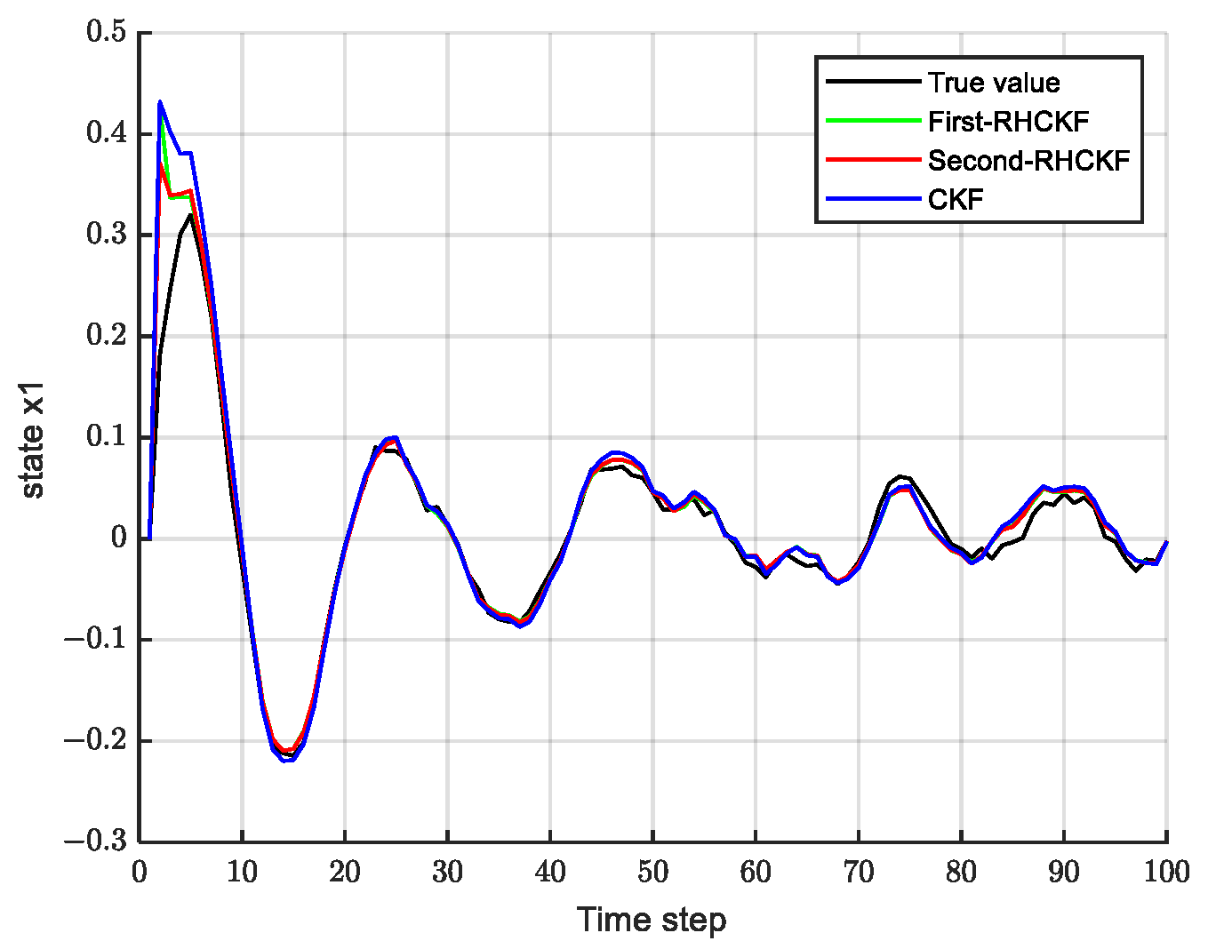
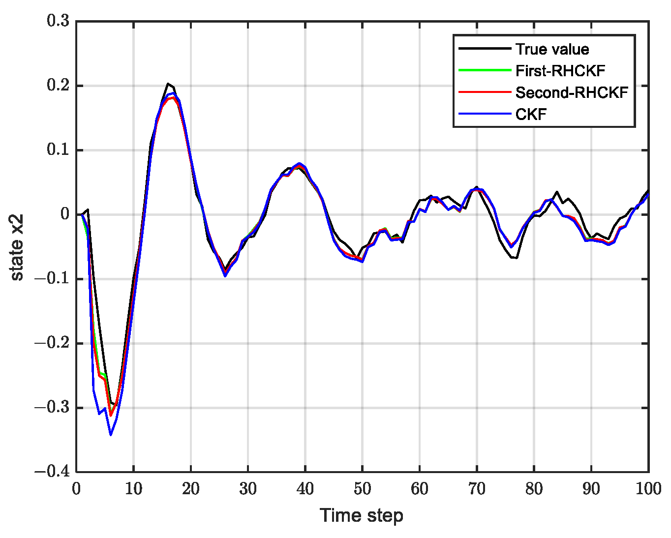
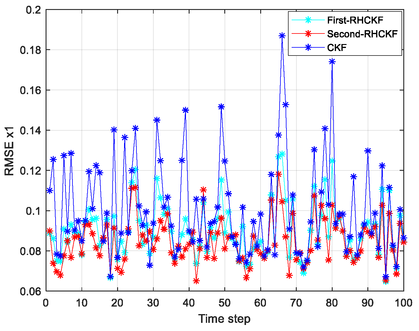
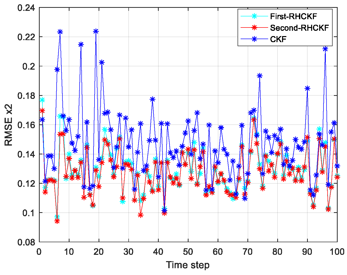
5.1. Experiment I

Consider the system where the equation of state is a two-dimensional nonlinear equation and the measurement equation is the one-dimensional under-measured nonlinear equation

$$\left[\begin{array}{l}{x}_1(k+1)\\ x_2(k+1)\end{array}\right]=\left[\begin{array}{l}0.85x_1(k)+0.5x_2(k)+0.5\sin (\gamma x_1(k))\\ -0.5x_1(k)+0.5\sin (\mu x_2(k))\end{array}\right]+\left[\begin{array}{l}{w}_1(k)\\ w_2(k)\end{array}\right]$$

(72)

$$z(k+1)=2\sin (x_1(k+1))+\sin (x_2(k+1))+v(k+1)$$

(73)

where the white noise is set to $w(k)\sim N\left[0,Q\right]$; $v(k+1)\sim N\left[0,R\right]$; $Q=diag\{0.01,0.01\}$; $R=0.01$; and the initial values of the experimental parameters are ${\widehat{x}}_0={\left[0.1,\hspace{0.17em}0.1\right]}^T$, $P_0=2\times diag(1,\hspace{0.17em}1)$, and $\gamma =1$, respectively.

From Figure 1 and Figure 2, it can be seen that each component of the state estimation can effectively follow the true state component, and Figure 3 and Figure 4 show the results of the root mean square error (RMSE) for 100 steps. Compared with the CKF, the RHCKF proposed in this paper has a better estimation effect.

From Figure 3 and Figure 4 and

Table 1. Comparison of estimation errors.

Methodologies	${\mathit{x}}_1$	${\mathit{x}}_2$
CKF	0.0967	0.1375
First-order RHCKF	0.0854	0.1281
VS CKF	13.23%	7.33%
Second-order RHCKF	0.0826	0.1272
VS CKF	17.07%	8.09%

, it can be seen that the average estimation errors of the first-order RHCKF for the target state are 0.0854 and 0.1281, respectively; that those of the second-order RHCKF for the target state are 0.0826 and 0.1272, respectively; that the improvements in the first-order RHCKF in comparison with the CKF are 13.23% and 7.33%; and that the improvements in the second-order RHCKF in comparison with the CKF are 17.07% and 8.09%. Moreover, the first-order RHCKF is more effective than the second-order RHCKF in improving the CKF because the first-order rounding error already contains most of the error information, and the second-order rounding error contains very little information, and the RHCKF is able to utilize more information of the model. The RHCKF takes into account the rounding error information in the process of approximating the nonlinear system of the sampled values, and it can utilize more information of the model compared to the CKF, so the filtering performance is also higher.

5.2. Experiment II

Consider a system with a nonlinear equation of state in two dimensions and a nonlinear equation of measurement in two dimensions.

$$\left[\begin{array}{l}{x}_1(k+1)\\ x_2(k+1)\end{array}\right]=\left[\begin{array}{l}0.85x_1(k)+0.5x_2(k)+0.5\sin (\gamma x_1(k))\\ -0.5x_1(k)+0.5\sin (\mu x_2(k))\end{array}\right]+\left[\begin{array}{l}{w}_1(k)\\ w_2(k)\end{array}\right]$$

(74)

$$\left[\begin{array}{l}{z}_1(k+1)\\ z_2(k+1)\end{array}\right]=\left[\begin{array}{l}\sin (x_1(k+1))\\ \sin (x_2(k+1))\end{array}\right]+\left[\begin{array}{l}{v}_1(k+1)\\ v_2(k+1)\end{array}\right]$$

(75)

where the white noise is set to $w(k)\sim N\left[0,Q\right]$; $v(k+1)\sim N\left[0,R\right]$; $Q=diag\{0.01,0.01\}$; $R=diag\{0.01,0.01\}$; and the initial values of the experimental parameters are ${\widehat{x}}_0={\left[0.1,\hspace{0.17em}0.1\right]}^T$, $P_0=2\times diag(1,\hspace{0.17em}1)$, and $\gamma =1$, respectively.

For a two-dimensional nonlinear system, Figure 5 and Figure 6 show the filtering effects of several filtering methods, and Figure 7 and Figure 8 show the results of the root mean square error (RMSE) for 100 steps. Combining the data in

Table 2. Performance comparison of different algorithms.

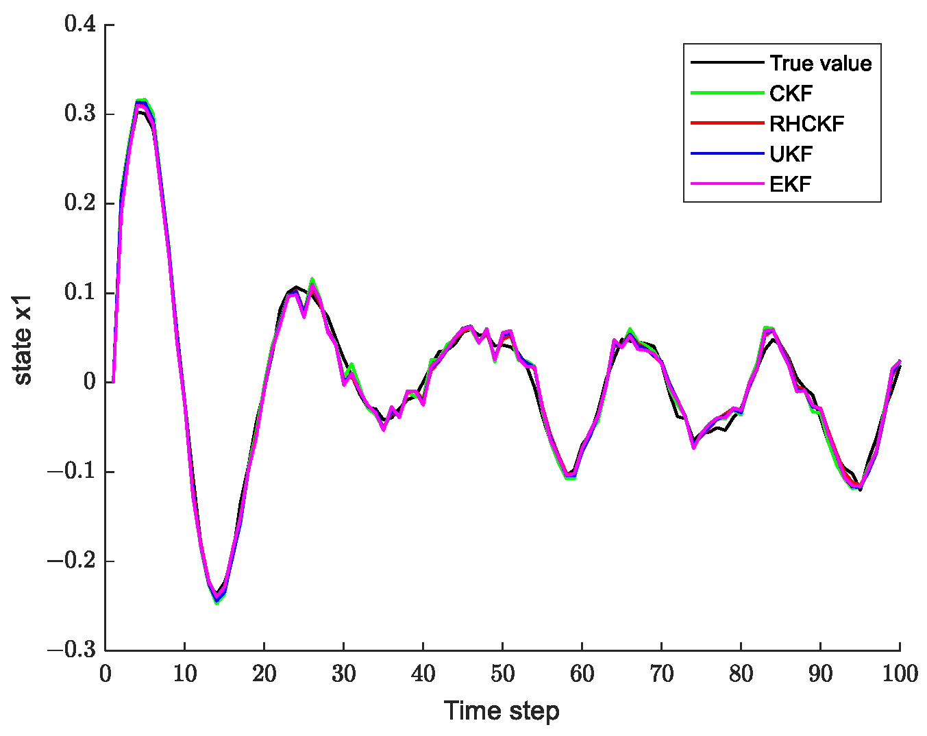
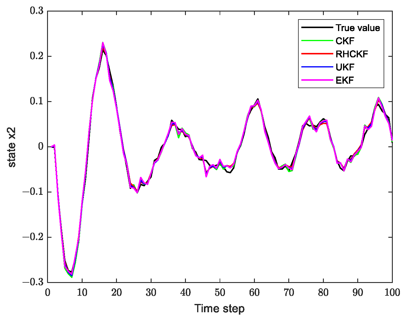
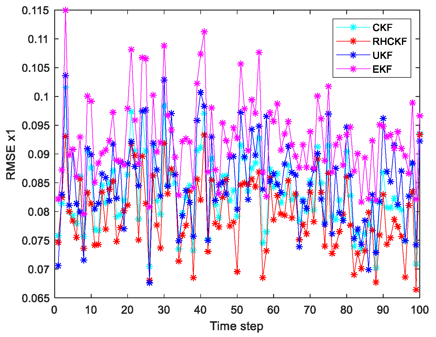
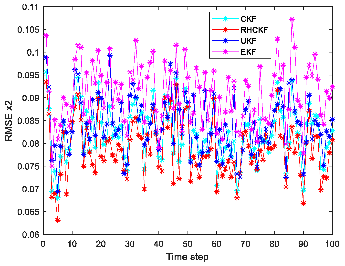
	RMSE	EKF	UKF	CKF	RHCKF	VS EKF	VS UKF	VSCKF
state	$x_1$	0.0928	0.0874	0.0863	0.0821	13.03%	6.45%	5.11%
	$x_2$	0.0985	0.0942	0.0935	0.0910	8.24%	3.51%	2.74%

, it can be seen that the estimation accuracy of the algorithm in this paper has been significantly improved regardless of the estimation of the state.

The dataa in Table 2 show that the estimated root mean square errors of the RHCKF algorithm in this paper are 0.0821 and 0.0910, respectively, which are significantly improved compared to the estimation accuracy of the EKF, UKF and CKF. Among them, the most improved was the EKF: $x_1=13.03\%$ and $x_2=8.24\%$.

There is a lower bound for the unbiased estimator of the minimum variance of the state of the nonlinear filtering algorithm, which is commonly measured by the Cramer–Rao lower bound limit in practice. The simulation results show that, compared with the traditional CKF, the root mean square error of the state of the proposed RHCKF is closer to that of the Cramer–Rao lower bound, and the filtering performance is also better than that of the CKF, so the RHCKF is an effective new method for state estimation.

6. Conclusions

Aiming at discrete-time nonlinear dynamic system, the traditional CKF cannot estimate the nonlinear model accurately, and these errors will have an impact on the estimation accuracy; for this reason, this paper firstly proposes a method to improve the estimation accuracy of the CKF by using the statistical properties of the rounding error. As the number of orders of the rounding error utilized increases, the more the approximation of the nonlinear function is enhanced, which means that there is less information about the rounding error. At the same time, from the point of view of state estimation, the less the rounding error, the more information can be utilized to design the filter, and the better the estimation of the filter will be. Finally, a higher-order extended cubature Kalman filter, based on the statistical characteristics of the system rounding error, was designed. The simulation experiment shows that, compared with the typical nonlinear filtering of the EKF, UKF and CKF, this method has achieved better estimation results, and the filtering accuracy has been significantly improved, providing a new solution to the problem of state estimation.

Although the method in this paper has achieved good filtering results, there are still areas for improvement. We have only analyzed the case where the observation equations of the nonlinear model are linear, and not the case where both the equation of state and the observation equations are nonlinear, both of which need to take advantage of the presence of rounding errors, which needs to be investigated in the future. In addition, a Bayesian approach (Idrovo-Aguirre & Contreras-Reyes, 2022) for an extended cubature Kalman filter can be addressed in a further work [22]. These are the key points and difficulties of the next step of research.

References

- Li, L.-Q.; Zhao, D.; Luo, C.-D. A Novel Interacting TS Fuzzy Multiple Model by Using UKF for Maneuvering Target Tracking. In Proceedings of the 2019 22th International Conference on Information Fusion (FUSION), Ottawa, ON, Canada, 2–5 July 2019; pp. 1–7. [Google Scholar]
- Meles, M.; Rajasekaran, A.; Mela, L.; Ruttik, K.; Jäntti, R. Impact of carrier frequency offset and phase noise on the steering vector for 3D drone localization based on angle of arrival (AOA). In Proceedings of the 2023 16th International Conference on Signal Processing and Communication System (ICSPCS), Bydgoszcz, Poland, 6–8 September 2023; pp. 1–6. [Google Scholar]
- Ito, K.; Xiong, K. Gaussian filters for nonlinear filtering problems. IEEE Trans. Autom. Control 2000, 45, 910–927. [Google Scholar] [CrossRef]
- Yuan, Y.; Zhou, D.; Li, J.; Lou, C. Time-varying parameters estimation with adaptive neural network EKF for missile-dual control system. J. Syst. Eng. Electron. 2024, 1–12. [Google Scholar] [CrossRef]
- Arellano-Valle, R.B.; Contreras-Reyes, J.E.; Quintero, F.O.L.; Valdebenito, A. A skew-normal dynamic linear model and Bayesian forecasting. Comput. Stat. 2019, 34, 1055–1085. [Google Scholar] [CrossRef]
- Cheng, C.; Wang, W.; Meng, X.; Shao, H.; Chen, H.J. Sigma-Mixed Unscented Kalman Filter-based Fault Detection for Traction Systems in High-speed Trains. Chin. J. Electron. 2023, 32, 982–991. [Google Scholar] [CrossRef]
- Pagoti, S.K.; Vemuri, S.I.D. Development and performance evaluation of Correntropy Kalman Filter for improved accuracy of GPS position estimation. Int. J. Intell. Netw. 2022, 3, 1–8. [Google Scholar] [CrossRef]
- Bucy, R.S.; Senne, K.D. Digital synthesis of non-linear filters. J. Autom. 1971, 7, 287–298. [Google Scholar] [CrossRef]
- Julier, S.J.; Uhlmann, J.K. Unscented filtering and nonlinear estimation. Proc. IEEE 2004, 92, 401–422. [Google Scholar] [CrossRef]
- Zhou, W.; Hou, J. A new adaptive high-order unscented Kalman filter for improving the accuracy and robustness of target tracking. IEEE Access 2019, 7, 118484–118497. [Google Scholar] [CrossRef]
- Wang, X.-X.; Pan, Q.; Huang, H.; Gao, A. Overview of deterministic sampling filtering algorithms for nonlinear system. Control Decis. 2012, 27, 801–812. [Google Scholar]
- Huber, M.F.; Hanebeck, U.D. Gaussian filter based on deterministic sampling for high quality nonlinear estimation. IFAC Proc. Cuba 2008, 41, 13527–13532. [Google Scholar] [CrossRef]
- Tian, Y.; Huang, Z.; Tian, J.; Li, X. State of charge estimation of lithium-ion batteries based on cubature Kalman filters with different matrix decomposition strategies. Energy 2022, 238, 121917. [Google Scholar] [CrossRef]
- Li, H.; Sun, H.; Chen, B.; Shen, H.; Yang, T.; Wang, Y.; Jiang, H.; Chen, L. A cubature Kalman filter for online state-of-charge estimation of lithium-ion battery using a gas-liquid dynamic model. J. Energy Storage 2022, 53, 105141. [Google Scholar] [CrossRef]
- Peng, J.; Luo, J.; He, H.; Lu, B. An improved state of charge estimation method based on cubature Kalman filter for lithium-ion batteries. Appl. Energy 2019, 253, 113520. [Google Scholar] [CrossRef]
- Jia, B.; Xin, M.; Cheng, Y. High-degree cubature Kalman filter. Automatica 2013, 49, 510–518. [Google Scholar] [CrossRef]
- Genz, A. Fully symmetric interpolatory rules for multiple integrals over hyper-spherical surfaces. J. Comput. Appl. Math. 2003, 157, 187–195. [Google Scholar] [CrossRef]
- He, J.; Sun, C.; Zhang, B.; Wang, P. Maximum correntropy square-root cubature Kalman filter for non-Gaussian measurement noise. IEEE Access 2020, 8, 70162–70170. [Google Scholar] [CrossRef]
- Zhang, L.; Cui, N.; Yang, F.; Lu, F.; Lu, B. High-degree cubature Kalman filter and its application in target tracking. J. Harbin Eng. Univ. 2016, 37, 573–578. [Google Scholar]
- Yang, H.; Wang, B.; He, J. Adaptive cubature Kalman filter for unknown noise covariance. J. Air Force Eng. Univ. 2021, 22, 42–47. [Google Scholar]
- Arasaratnam, I.; Haykin, S. Cubature kalman filters. IEEE Trans. Autom. Control 2009, 54, 1254–1269. [Google Scholar] [CrossRef]
- Idrovo-Aguirre, B.J.; Contreras-Reyes, J.E. Bayesian monthly index for building activity based on mixed frequencies: The case of Chile. J. Econ. Stud. 2022, 49, 541–557. [Google Scholar] [CrossRef]