Optimizing Allocation Rules in Discrete and Continuous Discriminant Analysis

Abstract

This paper presents an approach for the study of probabilistic outcomes in experiments with multiple possible results. An approach to obtain confidence ellipsoids for the vector of probabilities, which represents the likelihood of specific results, for both discrete and continuous discriminant analysis, is presented. The obtention of optimal allocation rules, in order to reduce the allocation costs is investigated. In the context of discrete discriminant analysis, the approach focuses on assigning elements to specific groups in an optimal way. Whereas in the continuous case, the approach involves determining the regions where each action is the optimal choice. The effectiveness of the proposed approach is examined with two numerical applications. One of them uses real data, while the other one uses simulated data.

1. Introduction

The process of allocating mixed data with several possible outcomes begins with the identification of the data. This includes identifying the type of data, the source of the data, and any relevant characteristics. Once the data have been identified, the next step is to determine the type of allocation that will be used. There are several different types of allocation, including random, manual, and automated allocation. Moreover, there are multiple methods for examining data with categorical outcomes. These methods include descriptive statistics, bivariate analyses, log-linear regression, multinomial logistic regression, discriminant analyses and quadratic discriminant analysis.

Descriptive statistics are used to summarize the characteristics of a data set.

Bivariate analysis is used to examine the relationship between two variables. In the case of categorical data, bivariate analysis consists of calculating the frequency or percentage of one variable for each category of the other variable.

The purpose of log-linear models is to study the relationship between an outcome variable and one or more explanatory variables, where the outcome variable is expressed as the logarithm of a linear combination of the explanatory variables. The log-linear model is a frequently used and simple structure for a contingency table, see Hand and Christen [1]. It is based on the same principle as the analysis of variance models, as outlined in Birch [2], Fienberg and Rinaldo [3] or Goodman [4], and is formed by calculating the logarithms of the cell probabilities. Examples of log-linear models with frequency tables can be found in Haberman [5].

On the other hand, Multinomial logistic regression is a generalized linear model that models the log-odds of the categorical response being true as a linear combination of predictor variables. It is a significant tool in statistical modelling and prediction, extending the capabilities of the binary logistic regression model to situations with more than two outcomes.

The goal of discriminant analysis is to classify individuals into distinct groups, maximizing the difference between groups and minimizing the variation within groups. Discriminant analysis has many advantages over the other mentioned methods. For example, it is able to identify and measure the effects of one or more independent variables on a dependent variable, making it a more powerful tool for predicting the outcome of a certain event. This method was first introduced by Sir Ronald Fisher in 1936, in Fisher [6], and is a popular research topic. Just to give a few examples over time, Rao [7] applied discriminant analysis to two types of problems confronted in biological research, while Friedman [8] proposed alternatives to the usual maximum likelihood estimates for the covariance matrices in linear and quadratic discriminant analysis, in small sample high-dimensional settings. McFarland et al. [9] used the theory of Bessel functions to derive stochastic representations for the exact distributions of the “plug-in” quadratic discriminant functions for classifying a newly obtained observation. Discriminant analysis was used in Perriere and Thioulouse [10] to separate Gram negative bacteria proteins according to their subcellular location. The problem of classifying an individual into one of several populations based on mixed nominal, continuous, and ordinal data was studied in Flury, Bourkai and Flury [11]. Modern research continues to find discriminant analysis helpful in problem-solving. For example, using dynamic feature extraction along with quadratic discriminant analysis classifier can significantly enhance fault classification and diagnosis in dynamic nonlinear processes, as demonstrated by Li, Jia, and Mao [12]. Furthermore, Tong et al. [13] demonstrated the effectiveness of discriminant analysis in their work on bearing fault diagnosis, representing a crucial development in fault diagnosis for dynamic nonlinear processes. For more information on discriminant analysis, see McLachlan [14].

Discriminant analysis can be divided into two categories: continuous and discrete. In the continuous case, the predictor variables are continuous and the output of the analysis is a continuous function. In the discrete case, the predictor variables are discrete and the output of the analysis is a classification. In both cases, discriminant analysis is used to find the optimal allocation rules. In the continuous case, the optimal allocation rule is determined by finding the optimal separating hyperplane which maximizes the difference between the groups. In the discrete case, the optimal allocation rule is determined by finding the optimal decision tree, which maximizes the accuracy of the classification.

A unified approach, providing optimal allocation rules to minimize expected costs for both continuous and mixed cases, is presented in Ferreira et al. [15]. We will follow this last approach.

Our goal is to obtain confidence ellipsoids for the vector of probabilities, $\mathit{p}$, of getting particular results in an experiment with m possible outcomes. Through duality, we will also test hypotheses. In addition, we will use support planes for ellipsoids, see Schott [16], to obtain simultaneous confidence intervals for these probabilities. Moreover, we will generalize these results to vectors

$$\mathbf{\Psi }=\mathit{G}\mathit{p},$$

(1)

where $\mathit{G}$ is a known matrix. Furthermore, we will show how to obtain optimal allocation rules, in order to reduce the allocation costs, first for the discrete case and then for the continuous case.

The rest of this paper is organized as follows. The next section, for preliminary results, is divided in two subsections. In the first one, we provide a simplified form of the continuous mapping theorem, CMT, based on Kallenberg [17]. This theorem will grant us the ability to derive confidence ellipsoids from the $N\left(\right|\mathit{0},W\left(\mathit{p}\right))$ distribution in the second subsection, where we will follow the approach of Scheffé [18]. Section 3 begins with the study of individual samples, followed by the study of pairs and structured families of independent samples. These samples refer to the treatments of a fixed effects experiment. The optimal allocation rules will be obtained in Section 4. Section 5 contains two numerical applications. The first, referring to the discrete case and using real data; the second, referring to the continuous case and using simulated data. We end the paper with some conclusions.

2. Preliminary Results

2.1. Asymptotic Distributions

The Central Limit Theorem, CLT, serves as a fundamental result in probability theory and statistics, providing insights into the behavior of sample averages. Let ${\mathit{Y}}_n$ be a sequence of random variables that converges in distribution to a limiting random variable $\mathit{Y}$, denoted as ${\mathit{Y}}_n\stackrel{d}{\to }\mathit{Y}$. Additionally, consider continuous functions $g\left({\mathit{Y}}_n\right)$ and $g\left(\mathit{Y}\right)$. The CLT, as established by Kallenberg [17], asserts that under these conditions, $g\left({\mathit{Y}}_n\right)$ converges in distribution to $g\left(\mathit{Y}\right)$, i.e., $g\left({\mathit{Y}}_n\right)\stackrel{d}{\to }g\left(\mathit{Y}\right)$.

Moreover, if the convergence in distribution of ${\mathit{Y}}_n$ to $\mathit{Y}$, given by $F_{{\mathit{Y}}_n}\left(\mathit{y}\right)\to F_{\mathit{Y}}\left(\mathit{y}\right)$, is uniform on a compact set L, then the convergence in distribution of $g\left({\mathit{Y}}_n\right)$ to $g\left(\mathit{Y}\right)$ is also uniform on the same set L. This uniform convergence property is valuable in understanding the stability of the distributional characteristics of the transformed random variables.

Further insights can be gained by considering the continuity of the function g. If g is a continuous function, then for any given $ϵ>0$, there exists a compact set $K\left(ϵ\right)$ such that the probability measure associated with $F_{{\mathit{Y}}_n}\left(\mathit{y}\right)$, denoted as ${\varphi }_n(.)$, satisfies ${\varphi }_n\left(K\left(ϵ\right)\right)\ge 1-ϵ$. Notably, the Cartesian product

$$\begin{array}{c}\hfill \dot{K}\left(ϵ\right)=K\left(ϵ\right)\times L\end{array}$$

(2)

is also a compact set. Consequently, the convergence in distribution of $g\left({\mathit{Y}}_n\right)$ to $g\left(\mathit{Y}\right)$ is uniform on the set $\dot{K}\left(ϵ\right)$.

In summary, the asymptotic distribution of $g\left({\mathit{Y}}_n\right)$ can be expressed as $F_{g\left(\mathit{Y}\right)}\left(\mathit{x}\right)$, provided that $\mathit{x}$ is a point of continuity for $F_{g\left(\mathit{Y}\right)}$. This convergence is established through the concept of weak convergence of probability measures, highlighting the broader applicability of the CLT in understanding the behavior of transformed random variables in a distributional sense.

2.2. Confidence Ellipsoids

Confidence ellipsoids serve as valuable tools for visualizing and quantifying uncertainty in multivariate data, providing insights into the variability of observations. These ellipsoids are particularly useful for testing hypotheses, constructing simultaneous confidence intervals, and making predictions in statistical analysis.

Consider a set of observations modeled by the linear equation $\mathit{Y}=\mathit{X}\mathit{\beta }+ϵ$, where $\mathit{X}$ is a design matrix, $\mathit{\beta }$ is a vector of fixed effects, and $ϵ$ is a vector of errors. The associated confidence ellipsoid, denoted as ${\mathit{E}}_q$, can be expressed as

$${\mathit{E}}_q=\{\mathit{Y}-\mathit{\mu }\in \Omega :{(\mathit{Y}-\mathit{\mu })}^{\top }{\mathit{C}}^{-1}(\mathit{Y}-\mathit{\mu })\le x_{h,1-q}\},$$

(3)

where $\mathit{\mu }=\mathit{X}\mathit{\beta }$ and $\mathit{C}={\mathit{X}}^{\top }\mathit{X}$. Here, $\Omega$ represents the feasible region of the ellipsoid, and $x_{h,1-q}$ is a critical value from a chi-square distribution with h degrees of freedom, ensuring a desired confidence level $1-q$.

The confidence ellipsoid ${\mathit{E}}_q$ possesses notable properties. Firstly, it is a convex set, implying that any point within the ellipsoid is a convex combination of points on its boundary. This property facilitates a comprehensive understanding of the distribution of observations.

Secondly, the confidence ellipsoid aids in constructing simultaneous confidence intervals. For a vector of interest, $\mathit{\tau }$, the simultaneous confidence interval for ${\mathit{\mu }}^{\top }\mathit{Y}$ is given by

$${\mathit{\tau }}^{\top }(\mathit{Y}-\mathit{\mu })\le \sqrt{x_{h,1-q}{\mathit{\tau }}^{\top }\mathit{C}\mathit{\tau }}.$$

(4)

This interval provides a range for the linear combination ${\mathit{\tau }}^{\top }\mathit{Y}$ with a specified level of confidence.

Finally, confidence ellipsoids are instrumental in hypothesis testing. Consider the following null hypothesis:

$$H_0:{\mathit{\tau }}^{\top }\mathit{\mu }=a_0.$$

(5)

If the hypothesis $H_0$ is true, then ${\mathit{E}}_q$ will contain the point ${(\mathit{Y}-\mathit{\mu })}_{a_0}=({\mathit{\tau }}^{\top }\mathit{Y}-{\mathit{\tau }}^{\top }\mathit{\mu })$; otherwise, the hypothesis is rejected.

3. Inference

In statistical inference, we often encounter experiments with multiple possible outcomes, each associated with a certain probability. To quantify the likelihood of obtaining specific results in such experiments, given the probabilities $p_1,\dots ,p_m$ of each outcome, and the observed frequencies $n_1,\dots ,n_m$ in n trials, we can employ the following probability function:

$$pr\left(\bigcap _{i=1}^m(N_i=n_i)\right)=\frac{n!}{{\prod }_{i=1}^m{n}_i!}\prod _{i=1}^m{p}_i^{n_i}\stackrel{d}{\to }M\left(\right|n,p),$$

(6)

where M represents a singular multivariate distribution.

Consider the probability vector $\mathit{p}=(p_1,\dots ,p_m)$, and define the vector of estimators:

$${\tilde{\mathit{p}}}_n=({\tilde{p}}_{n,1},\dots ,{\tilde{p}}_{n,m}),$$

(7)

with ${\tilde{p}}_{n,i}=\frac{n_i}{n}$ for $i=1,\dots ,m$. These estimators represent the observed probabilities of each outcome. As the number of trials n approaches infinity, Wilks’ theorem, in Wilks [19], provides insight into the asymptotic behavior of the estimators:

$$\sqrt{n}({\tilde{\mathit{p}}}_n-\mathit{p})\stackrel{d}{\to }N(\mathit{0},W\left(\mathit{p}\right)),$$

(8)

where $\stackrel{d}{\to }$ denotes convergence in distribution, and $N(\mathit{0},W(\mathit{p}\left)\right)$ represents a normal distribution with zero mean vector and covariance matrix $W\left(\mathit{p}\right)$.

The covariance matrix $W\left(\mathit{p}\right)$ is defined as

$$W\left(\mathit{p}\right)=D\left(\mathit{p}\right)-\mathit{p}{\mathit{p}}^{\top },$$

(9)

where $D\left(\mathit{p}\right)$ is a diagonal matrix with the components of $\mathit{p}$ along its diagonal. The probabilities in the initial distribution can be estimated from the observed frequencies through maximum likelihood estimation, where each ${\tilde{p}}_{n,i}=\frac{n_i}{n}$ for $i=1,\dots ,m$. This result indicates that as the sample size grows, the distribution of the estimated probabilities becomes approximately normal, facilitating the application of classical statistical inference techniques. The covariance matrix $W\left(\mathit{p}\right)$ characterizes the variability in the estimates, and its asymptotic normality allows for the construction of confidence intervals and hypothesis tests based on the estimated probabilities ${\tilde{\mathit{p}}}_n$.

3.1. One Sample

Let ${\mathit{\alpha }}_1,\dots ,{\mathit{\alpha }}_m$ constitute an orthonormal basis for the orthogonal complement, ${\Omega }^{\perp }$, of $\Omega$. Then, we can write

$$W\left({\tilde{\mathit{p}}}_n\right)=\sum _{j=1}^m{v}_j{\mathit{\alpha }}_j{\mathit{\alpha }}_j^{\top },$$

(10)

where $v_j$ is the eigenvalue associated with ${\mathit{\alpha }}_j$, see Horn [20]. We can further decompose the matrix $W\left({\tilde{\mathit{p}}}_n\right)$ as

$$W\left({\tilde{\mathit{p}}}_n\right)=\sum _{j=1}^{m-1}{v}_i{\mathit{\alpha }}_j{\mathit{\alpha }}_j^{\top }+v_m{\mathit{\alpha }}_m{\mathit{\alpha }}_m^{\top }.$$

(11)

Let ${\mathit{\alpha }}_m$ be the eigenvector associated with the largest eigenvalue $v_m$. Then, we can write

$$W{\left({\tilde{\mathit{p}}}_n\right)}^{+}=\sum _{j=1}^{m-1}{v}_j^{-1}{\mathit{\alpha }}_j{\mathit{\alpha }}_j^{\top }+v_m^{-1}{\mathit{\alpha }}_m{\mathit{\alpha }}_m^{\top },$$

(12)

where + denotes the Moore–Penrose inverse, expressed as

$$W{\left({\tilde{\mathit{p}}}_n\right)}^{+}=\sum _{j=1}^m{v}_j^{-1}{\mathit{\alpha }}_j{\mathit{\alpha }}_j^{\top }.$$

(13)

According to Schott [16] and attending to the continuity of the Moore–Penrose inverse, if

$$W\left({\tilde{\mathit{p}}}_n\right)\stackrel{p}{\to }W\left(\mathit{p}\right),$$

(14)

where $\stackrel{p}{\to }$ denotes convergence in probability, then

$$W{\left({\tilde{\mathit{p}}}_n\right)}^{+}\stackrel{p}{\to }W{\left(\mathit{p}\right)}^{+}.$$

(15)

Moreover, the continuity of the Moore–Penrose inverse implies that the covariance matrix of the vector $\sqrt{n}({\tilde{\mathit{p}}}_n-\mathit{p})$, $/\Sigma \left(\sqrt{n}({\tilde{\mathit{p}}}_n-\mathit{p})\right)$ will converge in probability to $W\left(\mathit{p}\right)$,

$$/\Sigma \left(\sqrt{n}({\tilde{\mathit{p}}}_n-\mathit{p})\right)\stackrel{p}{\to }W\left(\mathit{p}\right).$$

(16)

Furthermore, the continuity of the Moore–Penrose inverse implies that, if $\mathit{c}$ is a vector, the inner product ${\mathit{c}}^{\top }W\left({\tilde{\mathit{p}}}_n\right)\mathit{c}$ will converge in probability to the inner product ${\mathit{c}}^{\top }W\left(\mathit{p}\right)\mathit{c}$, i.e.,

$${\mathit{c}}^{\top }W\left({\tilde{\mathit{p}}}_n\right)\mathit{c}\stackrel{p}{\to }{\mathit{c}}^{\top }W\left(\mathit{p}\right)\mathit{c}$$

(17)

and the variance of the vector $\sqrt{n}{\mathit{c}}^{\top }({\tilde{\mathit{p}}}_n-\mathit{p})\mathit{c}$ will also converge in probability to the inner product ${\mathit{c}}^{\top }W\left(\mathit{p}\right)\mathit{c}$, i.e.,

$$Var\left(\sqrt{n}{\mathit{c}}^{\top }({\tilde{\mathit{p}}}_n-\mathit{p})\mathit{c}\right)\stackrel{p}{\to }{\mathit{c}}^{\top }W\left(\mathit{p}\right)\mathit{c}.$$

(18)

These properties of the Moore–Penrose inverse can be used to draw statistical inference from the data. For example, the covariance matrix of the vector $\sqrt{n}({\tilde{\mathit{p}}}_n-\mathit{p})$ can be used to estimate the variance of the vector $\mathit{p}$, and the inner product ${\mathit{c}}^{\top }W\left({\tilde{\mathit{p}}}_n\right)\mathit{c}$ can be used to estimate the inner product ${\mathit{c}}^{\top }W\left(\mathit{p}\right)\mathit{c}$. Besides this, we have

$$\left\{\begin{array}{c}\hfill \sqrt{n}({\tilde{\mathit{p}}}_n-\mathit{p})\curvearrowright N(\mathit{0},W\left(\mathit{p}\right))\hfill \\ \hfill \sqrt{n}({\mathit{c}}^{\top }{\tilde{\mathit{p}}}_n-{\mathit{c}}^{\top }\mathit{p})\curvearrowright N(\mathit{0},{\mathit{c}}^{\top }W\left(\mathit{p}\right)\mathit{c})\hfill \end{array}\right.;$$

(19)

see Tsui [21]. We can then make use of the central limit theorem to show that

$$\sqrt{n}\frac{{\mathit{c}}^{\top }({\tilde{\mathit{p}}}_n-\mathit{p})\mathit{c}}{\sqrt{{\mathit{c}}^{\top }W\left({\tilde{\mathit{p}}}_n\right)\mathit{c}}}\curvearrowright N(0,1).$$

(20)

Using this result, we can construct a confidence interval for ${\mathit{c}}^{\top }\mathit{p}$, with confidence level $(1-q)$, given by

$$pr\left({\mathit{c}}^{\top }{\tilde{\mathit{p}}}_n-z_q\sqrt{\frac{{\mathit{c}}^{\top }W\left({\tilde{\mathit{p}}}_n\right)\mathit{c}}{n}}\le {\mathit{c}}^{\top }\mathit{p}\le {\mathit{c}}^{\top }{\tilde{\mathit{p}}}_n+z_q\sqrt{\frac{{\mathit{c}}^{\top }W\left({\tilde{\mathit{p}}}_n\right)\mathit{c}}{n}}\right)\to 1-q.$$

(21)

We may then use duality to test the hypothesis

$$H_0\left(\mathit{c}\right):{\mathit{c}}^{\top }\mathit{p}={\mathit{c}}^{\top }{\mathit{p}}_0$$

(22)

at the limit q. This method is useful for testing hypotheses about parameters in a variety of different models, including linear mixed models.

3.2. Pair of Samples

We denote $M\left(\right|m\left(l\right),\mathit{p}\left(l\right))$ as the singular multivariate distribution for a pair of independent samples, $l=1,2$, with $\mathit{p}\left(l\right)=(p_1\left(l\right),\dots ,p_m\left(l\right))$ and $p_i\left(l\right)\ge 0$. Thus, distributions and the corresponding statistics, such as estimators, will be independent.

We have

$$\sqrt{n\left(l\right)}\left(\tilde{\mathit{p}}\left(l\right)-\mathit{p}\left(l\right)\right)\curvearrowright N\left(\right|\mathit{0},W\left(\mathit{p}\left(l\right)\right)).$$

(23)

We can also take the difference between each of the $p_i\left(1\right)$ and $p_i\left(2\right)$, $i=1,\dots ,m$, and end up with unbiased estimators for $q_i$, as follows:

$${\tilde{q}}_i={\tilde{p}}_i\left(1\right)-{\tilde{p}}_i\left(2\right),i=1,\dots ,m.$$

(24)

If $\frac{n\left(2\right)}{n\left(1\right)}\to r$, we will have

$$\left\{\begin{array}{c}\hfill \frac{n\left(1\right)}{n}\to \frac{1}{1+r}\hfill \\ \hfill \frac{n\left(2\right)}{n}\to \frac{r}{1+r}\hfill \end{array}\right.,$$

(25)

with $n=n\left(1\right)+n\left(2\right)$. So,

$$\left\{\begin{array}{c}\hfill Var\left(\sqrt{n}{\tilde{p}}_i\left(1\right)\right)\to (r+1)p_i\left(1\right)(1-p_i\left(1\right))\hfill \\ \hfill Var\left(\sqrt{n}{\tilde{p}}_i\left(2\right)\right)\to \frac{r+1}{r}{p}_i\left(2\right)(1-p_i\left(2\right))\hfill \end{array}\right.,i=1,\dots ,m$$

(26)

and, given the independence of the two samples,

$$Var\left(\sqrt{n}{\tilde{q}}_i\right)\to (r+1)\left[p_i\left(1\right)(1-p_i\left(1\right))+\frac{1}{r}{p}_i\left(2\right)(1-p_i\left(2\right))\right],i=1,\dots ,m.$$

(27)

When $r\to 0$, the variance of $\sqrt{n}{\tilde{q}}_i$ tends to zero, so it becomes an unbiased estimator. The same is true for $r\to \infty$. To compare the two multivariate distributions, $M\left(\right|m\left(1\right),\mathit{p}\left(1\right))$ and $M\left(\right|m\left(2\right),\mathit{p}\left(2\right))$, we can use the Hotelling’s $T^2$ statistic to measure the distance between the two distributions:

$$T^2=n{\left(\tilde{\mathit{p}}\left(1\right)-\tilde{\mathit{p}}\left(2\right)\right)}^{T}W{\left(\mathit{p}\left(1\right)\right)}^{-1}\left(\tilde{\mathit{p}}\left(1\right)-\tilde{\mathit{p}}\left(2\right)\right).$$

(28)

It is well known that if

$$\frac{n\left(2\right)}{n\left(1\right)}\to r,$$

(29)

then

$$T^2\curvearrowright {\chi }_{m-1}^2\left(r\right).$$

(30)

Now, reasoning as in the previous subsection, it may be shown that

$$\frac{\sqrt{n}({\tilde{q}}_i-q_i)}{\sqrt{(r+1){\tilde{p}}_i\left(1\right)(1-{\tilde{p}}_i\left(1\right))+\frac{1}{r}{\tilde{p}}_i\left(2\right)(1-{\tilde{p}}_i\left(2\right))}}\curvearrowright N\left(\right|0,1),i=1,\dots ,m,$$

(31)

and so

$$\begin{array}{c}\hfill pr\left[{\tilde{q}}_i-z_q\sqrt{(r+1)\left({\tilde{p}}_i\left(1\right)(1-{\tilde{p}}_i\left(1\right))+\frac{1}{r}{\tilde{p}}_i\left(2\right)(1-{\tilde{p}}_i\left(2\right))\right)}\le q_i\right.\\ \hfill \le \left.{\tilde{q}}_i+z_q\sqrt{(r+1)\left({\tilde{p}}_i\left(1\right)(1-{\tilde{p}}_i\left(1\right))+\frac{1}{r}{\tilde{p}}_i\left(2\right)(1-{\tilde{p}}_i\left(2\right))\right)}\right]\le 1-q,i=1,\dots ,m.\end{array}$$

(32)

Thus, through duality, we get a $1-q$ limit level test for

$$H_0\left(q_{0,i}\right):q_i=q_{0,i},i=1,\dots ,m.$$

(33)

In addition,

$$\left\{\begin{array}{c}\hfill Var\left(\sqrt{n}{\mathit{c}}^{\top }\tilde{\mathit{p}}\left(1\right)\right)\to (r+1){\mathit{c}}^{\top }W\left(\mathit{p}\left(1\right)\right)\mathit{c}\hfill \\ \hfill Var\left(\sqrt{n}{\mathit{c}}^{\top }\tilde{\mathit{p}}\left(2\right)\right)\to \frac{r+1}{r}{\mathit{c}}^{\top }W\left(\mathit{p}\left(2\right)\right)\mathit{c}\hfill \end{array}\right.,$$

(34)

as $n\to \infty$, so that

$$Var\left(\sqrt{n}({\mathit{c}}^{\top }\tilde{\mathit{p}}\left(1\right)-{\mathit{c}}^{\top }\tilde{\mathit{p}}\left(2\right))\right)\underset{n\to \infty }{\to }(r+1){\mathit{c}}^{\top }\left[W\left(\mathit{p}\left(1\right)\right)+\frac{1}{r}W(\mathit{p}\left(2\right)\right]\mathit{c},$$

(35)

and that

$$\begin{array}{c}\hfill \frac{\sqrt{n}\left[({\mathit{c}}^{\top }\tilde{\mathit{p}}\left(1\right)-{\mathit{c}}^{\top }\tilde{\mathit{p}}\left(2\right))-({\mathit{c}}^{\top }\mathit{p}\left(1\right)-{\mathit{c}}^{\top }\mathit{p}\left(2\right))\right]}{\sqrt{(r+1)({\mathit{c}}^{\top }W\left(\tilde{\mathit{p}}\left(1\right)\right)+\frac{1}{r}W\left(\tilde{\mathit{p}}\left(2\right)\right)\mathit{c})}}=\end{array}$$

(36)

$$\begin{array}{c}\hfill \frac{\sqrt{n}({\mathit{c}}^{\top }\tilde{\mathit{q}}-{\mathit{c}}^{\top }\mathit{q})}{\sqrt{(r+1)({\mathit{c}}^{\top }W\left(\tilde{\mathit{p}}\left(1\right)\right)+\frac{1}{r}W\left(\tilde{\mathit{p}}\left(2\right)\right)\mathit{c})}}\curvearrowright N\left(\right|0,1).\end{array}$$

(37)

Thus,

$$\begin{array}{c}\hfill pr\left({\mathit{c}}^{\top }\tilde{\mathit{q}}-z_q\sqrt{(r+1)({\mathit{c}}^{\top }W\left(\tilde{\mathit{p}}\left(1\right)\right)+\frac{1}{r}W\left(\tilde{p}\left(2\right)\right)\mathit{c})}\le {\mathit{c}}^{\top }\mathit{q}\le \right.\end{array}$$

(38)

$$\begin{array}{c}\hfill \left.{\mathit{c}}^{\top }\tilde{\mathit{q}}+z_q\sqrt{(r+1)({\mathit{c}}^{\top }W\left(\tilde{\mathit{p}}\left(1\right)\right)+\frac{1}{r}W\left(\tilde{p}\left(2\right)\right)\mathit{c})}\right)\to 1-q.\end{array}$$

(39)

And, using duality once again, we can obtain limit level q tests for

$$H_0\left({\mathit{c}}^{\top }\mathit{q}\right):{\mathit{c}}^{\top }\mathit{q}=d_l,l=1,2.$$

(40)

3.3. Structured Families of Samples

Let us consider d treatments of fixed-effects designs, with a total of

$$n=\sum _{l=1}^{d}n\left(l\right)$$

(41)

individuals, and d independent samples. This configuration is referred to as a structured family, and the distributions of the samples,

$$M\left(\right|n\left(l\right),\mathit{p}\left(l\right)),l=1,\dots ,d,$$

(42)

with $\mathit{p}\left(l\right)=(p_1\left(l\right),\dots ,p_m\left(l\right))$, $l=1,\dots ,d$, and $p_i\left(l\right)\ge 0$, $i=1,\dots ,m$, $l=1,\dots ,d$, characterize it. Moreover, consider

$$\frac{n\left(l\right)}{n}\to r\left(l\right),l=1,\dots ,d.$$

(43)

Now, we will have

$${\dot{\mathit{X}}}_n\left(l\right)=\frac{n}{r\left(l\right)}{\left({\tilde{\mathit{p}}}_{n\left(l\right)}\left(l\right)-\mathit{p}\left(l\right)\right)}^{\top }{W}^{+}\left({\mathit{p}}_l\right)\left({\tilde{\mathit{p}}}_{n\left(l\right)}-\mathit{p}\left(l\right)\right)\to G\left(\right|m-1),l=1,\dots ,d,$$

(44)

where $G\left(\right|m-1)$ is the gamma distribution with a shape parameter of $m-1$ and a scale parameter of 1. So, with ${\dot{\mathit{X}}}_n=({\dot{\mathit{X}}}_n\left(1\right),\dots ,{\dot{\mathit{X}}}_n\left(d\right))$, given the independence of the ${\dot{\mathit{X}}}_n\left(l\right)$, $l=1,\dots ,d$, we have

$${\dot{\mathit{X}}}_n\curvearrowright G\left(\right|m-1),$$

(45)

with

$$\dot{G}\left(\mathit{x}\right|m-1)=\prod _{l=1}^{d}G\left(x_l\right|m-1),$$

(46)

whenever $\mathit{x}=(x_1,\dots ,x_d)$.

We now study the action of the factors in the base design, assuming that the hypotheses of absence of effects and interactions are linked to an orthogonal partition,

$${\mathcal{R}}^d={⊞}_{j=1}^m{\nabla }_j,$$

(47)

and that the row vectors of ${\mathit{A}}_j$ constitute an orthonormal basis for ${\nabla }_j$, $j=1,\dots ,m$. This leads to the hypotheses

$$H_{0,j}\left(\mathit{c}\right):{\mathit{A}}_j\eta \left(\mathit{c}\right)=\mathit{0},j=1,\dots ,m,$$

(48)

where $\eta \left(\mathit{c}\right)=({\mathit{c}}^{\top }\mathit{p}\left(1\right),\dots ,{\mathit{c}}^{\top }\mathit{p}\left(d\right))$.

More generally,

$$H_{0,j}\left(\mathit{c}\right):{\mathbf{\Psi }}_j\left(\mathit{c}\right)={\mathbf{\Psi }}_{0,j}\left(\mathit{c}\right),j=1,\dots ,m.$$

(49)

We have

$${\mathbf{\Psi }}_j\left(\mathit{c}\right)={\mathit{A}}_j\eta \left(\mathit{c}\right).$$

(50)

So, we will have

$$\tilde{\eta }\left(\mathit{c}\right)=({\mathit{c}}^{\top }\mathit{p}\left(1\right),\dots ,{\mathit{c}}^{\top }\mathit{p}\left(d\right)){\tilde{\mathbf{\Psi }}}_j\left(\mathit{c}\right)={\mathit{A}}_j\tilde{\eta }\left(\mathit{c}\right)\curvearrowright N\left(\right|{\mathbf{\Psi }}_j\left(\mathit{c}\right),{\mathit{A}}_{j}D\left(\mathit{c}\right){\mathit{A}}_j^{\top }),$$

(51)

where $D\left(\mathit{c}\right)$ is the diagonal matrix, with

$$\begin{array}{c}\hfill {\mathit{c}}^{\top }W\left(\mathit{p}\left(1\right)\right)\mathit{c},\dots ,{\mathit{c}}^{\top }W\left(\mathit{p}\left(d\right)\right)\mathit{c}\end{array}$$

(52)

along its diagonal, and the estimator is given by

$${\tilde{\Psi }}_j^{\top }\left(\mathit{c}\right){\mathit{A}}_j\mathit{D}\left(\mathit{c}\right){\left({\mathit{A}}_j^{\top }\right)}^{+}{\tilde{\Psi }}_j\left(\mathit{c}\right)\curvearrowright G\left(\right|g_j),j=1,\dots ,m.$$

(53)

Moreover, $x_{g_j,1-q}$ will be the critical value for a limit level q test for

$$H_{0,j}\left(\mathit{c}\right),j=1,\dots ,m.$$

(54)

4. Optimal Allocation Rules

4.1. The Discrete Case

Consider a set of populations combined together, each placed into different groups. A randomly selected sample of n elements from this mixture belongs to a specified population and class, denoted as $n_{i,j}$ for elements in class ${\S }_i$ and population $P_j$, with $i=1$ to w and $j=1$ to m.

Our objective is to determine an allocation rule that minimizes the overall cost of assigning elements to their respective populations. The cost of assigning an element from $P_j$ to $P_{j^{\prime }}$ is represented by $c_{j,j^{\prime }}$.

Let $E_{i,j}$ be the event that a randomly chosen element belongs to ${\S }_i$ and $P_j$, with $E_{i,·}$ [$E_{·,j}$] representing the event that a randomly chosen element belongs to ${\S }_i$ [$P_j$]. Define

$$\left\{\begin{array}{c}\hfill p_{i,j}=pr\left(E_{i,j}\right)\hfill \\ \hfill p_{i,·}=pr\left(E_{i,·}\right)\hfill \\ \hfill p_{·,j}=pr\left(E_{·,j}\right)\hfill \end{array}\right.,$$

(55)

for $i=1,\dots ,w$ and $j=1,\dots ,m$. Additionally, introduce conditional probabilities

$$\left\{\begin{array}{c}\hfill p_{i|j}=pr\left(E_{i,·}\right|E_{·,j})\hfill \\ \hfill p_{j|i}=pr\left(E_{·,j}\right|E_{i,·})\hfill \end{array}\right.,$$

(56)

for $i=1,\dots ,w$ and $j=1,\dots ,m$.

If the elements located in ${\S }_i$ are assigned to $P_j$, $i=1,\dots ,w$, $j=1,\dots ,m$, the average cost is given by

$$c_{i\left(j\right)}=\sum _{j^{\prime }=1}^m{p}_{j^{\prime },i}{c}_{j^{\prime },j},i=1,\dots ,w,j=1,\dots ,m.$$

(57)

This leads to consistent estimators

$$\left\{\begin{array}{l}{\tilde{p}}_{i,j}=\frac{n_{i,j}}{n}\hfill \\ {\tilde{p}}_{i,·}=\sum _{j=1}^m{\tilde{p}}_{i,j}{\tilde{p}}_{·,j}\hfill \\ {\tilde{p}}_{i|j}=\frac{{\tilde{p}}_{i,j}}{{\tilde{p}}_{i,·}}\hfill \end{array}\right.,$$

(58)

as the sample size increases, and the estimated average cost

$${\tilde{c}}_i\left(j\right)=\sum _{j^{\prime }=1}^m{\tilde{p}}_{j^{\prime },i}{c}_{j^{\prime },j},i=1,\dots ,w,j=1,\dots ,m.$$

(59)

An optimum allocation for $x_i$ occurs if there exists a $j\left(i\right)$ such that $c_i\left(j\left(i\right)\right)<c_i\left(j\right)$ for $j\ne j\left(i\right)$, in which case

$$pr\left(\bigcap _{j\ne j\left(i\right)}({\tilde{c}}_i\left(j\left(i\right)\right)<{\tilde{c}}_i\left(j\right))\right)\underset{n\to \infty }{\to }1,i=1,\dots ,w.$$

(60)

Furthermore, if there is an optimum allocation for all $x_i$, $i=1,\dots ,w$,

$$pr\left(\bigcap _{i=1}^w\bigcap _{j\ne j\left(i\right)}{\tilde{c}}_i\left(j\left(i\right)\right)<{\tilde{c}}_i\left(j\right)\right)\underset{n\to \infty }{\to }1.$$

(61)

Discriminant analysis is consistent, indicating that the probability of the allocation rule being optimal increases as the initial sample size grows to infinity. This holds true for all ${\S }_i$, with i ranging from 1 to w.

The global average cost of assigning elements of ${\S }_i$, $i=1,\dots ,w$, to $P_{j\left(i\right)}$ is given by

$$c_{.}=\sum _{i=1}^w{p}_i{c}_i\left(j\left(i\right)\right),$$

(62)

with the consistent estimator

$${\tilde{c}}_{.}=\sum _{i=1}^w{\tilde{p}}_i{c}_i\left(j\left(i\right)\right),$$

(63)

and the limit level $1-p$ confidence interval

$${\tilde{c}}_{.}\pm z_q^{\prime }\sqrt{{\mathit{d}}^{\top }W\left(\tilde{\mathit{p}}\right)\mathit{d}},$$

(64)

where $z_q^{\prime }$ is the critical value of a standard normal distribution at level $1-q$, and $\mathit{d}$ is the vector with all components null except the one with index $1+(i-1)j\left(i\right)$, $i=1,\dots ,w$, which is 1.

4.2. The Continuos Case

For each event ${\mathcal{A}}_i$, $i=1,\dots ,k$, that occurs when an element of $\mathcal{P}$ is randomly chosen to belong to ${\mathcal{P}}_i$, $i=1,\dots ,k$, the probability of the event is $p_i=pr\left({\mathcal{A}}_i\right)$. To determine the allocation, a partition of the observations vector $\mathit{X}\in {\mathbb{R}}^n$ is created such that each element is assigned to ${\mathcal{P}}_i$ when $\mathit{X}\in {\Omega }_i$, $i=1,\dots ,k$. The probability of assigning to ${\mathcal{P}}_j$ an element of ${\mathcal{P}}_i$ is denoted as $q_{i,j}$, $i=1,\dots ,k$ and $j=1,\dots ,k$, and is calculated from the densities of $\mathit{X}$ in the ${\mathcal{P}}_i$, $i=1,\dots ,k$. The expected cost of the decision is then determined by summing the product of the costs of each pair of events and their associated probabilities.

The average cost incurred by the decision will be equal to the sum of the probabilities multiplied by the expected cost for each action multiplied by the probability of that action. This can be expressed as the sum of integrals for each possible action over the region where that action is the optimal choice. That is,

$$\begin{array}{c}\hfill E\left(C\right)=\sum _{j=1}^k{\int \dots \int }_{{\Omega }_j}{g}_j\left(\mathit{x}\right)\prod _{l=1}^{n}d{x}_l,\end{array}$$

(65)

with

$$g_j\left(\mathit{x}\right)=\sum _{i=1}^k{p}_i{c}_{i,j}{f}_i\left(\mathit{x}\right);j=1,\dots ,k.$$

(66)

To minimize the expected cost, one must take the regions where each action is the optimal choice,

$${\Omega }_j=\{\mathit{x}:g_j\left(\mathit{x}\right)\le g_i\left(\mathit{x}\right),i=1,\dots ,k\};j=1,\dots ,k.$$

(67)

In the situation of identical decision costs, for which $c_{i,j}=c$, $i\ne j$, this is especially noteworthy. This means that

$$g_j\left(\mathit{x}\right)=c\sum _{i\ne j}{p}_i{f}_i\left(\mathit{x}\right)=c\sum _{i=1}^k{p}_i{f}_i\left(\mathit{x}\right)-c{p}_j{f}_j\left(\mathit{x}\right);j=1,\dots ,k,$$

(68)

and the sets

$${\Omega }_j=\{\mathit{x}:p_j{f}_j\left(\mathit{x}\right)\ge p_i{f}_i\left(\mathit{x}\right),i=1,\dots ,k\};j=1,\dots ,k.$$

(69)

are applicable. In addition, if $p_i=\frac{1}{k}$, $i=1,\dots ,k$, then

$${\Omega }_j=\{\mathit{x}:f_j\left(\mathit{x}\right)\ge f_i\left(\mathit{x}\right),i=1,\dots ,k\};j=1,\dots ,k.$$

(70)

This means that, given $\mathit{x}$, the population with the greatest probability will be chosen.

In summary, the expected cost associated with the decision can be expressed as a sum of integrals over the regions where each action is the optimal choice. This decision can be further simplified when the costs for each action are equal and the probabilities are the same. In this situation, the decision is simply to choose the population with the greatest probability.

5. Numerical Applications

5.1. The Discrete Case—An Application to Real Data

The purpose of this subsection is to illustrate the theory, relative to the discrete case. To do this, we use an application with real data, obtained from Instituto Superior Dom Bosco [22], related to the impact of four economic policies on greenhouse gas emissions: Policy A, Policy B, Policy C, and Policy D. The data were provided by the Instituto Superior Dom Bosco, and will be used to highlight the effectiveness of the discrimination rule in guiding resource allocation decisions.

Let us assume that for each region, the four policies have four distinct categories. This would create $4^4=256$ possible combinations. If our null hypothesis is true and all of the combinations are equally likely, then any given combination should have a probability of $\frac{1}{256}$.

We present a discrimination rule, which will classify regions into two groups, “High Emission” (Population 1) and “Low Emission” (Population 2), based on the values of the statistic:

$$v=|x_1-x_2|+|x_1-x_3|+|x_1-x_4|+|x_2-x_3|+|x_2-x_4|+|x_3-x_4|+1,$$

(71)

where each policy category has a value of 1, 2, 3, or 4.

The choice of this statistic is based on its ability to capture the differences between the four economic policies in terms of their impact on greenhouse gas emissions. By calculating the absolute differences between the categories of each policy and summing them, we obtain a single value that represents the overall dissimilarity between the policies. In addition, the use of the absolute differences ensures that the magnitude of the differences is taken into account, regardless of their direction. This is important in the context of evaluating policy effectiveness, as both positive and negative differences can contribute to the overall impact.

The collection of potential values for v is $\mathit{D}=\left\{1,4,5,7,8,9,10,12,13\right\}$. We use the values of $r_h={\displaystyle \frac{p_{h,1}}{p_{h,2}}},$$h\in \mathit{D}$ of the conditional probabilities and allocate to population 2 or 1 those with $v\in \mathit{D}\left(x\right)$ or $v\notin \mathit{D}\left(x\right)$, respectively.

Suppose $n_{h,l}$ denotes the number of elements with $v=h$ in population l. We can obtain the sample size for each population as follows:

$$\sum _{h\in \mathit{D}}{n}_{h,l},l=1,2$$

(72)

and the probability of obtaining $v=h$ in a randomly chosen element from that sample as

$${\displaystyle \frac{n_{h,l}}{{\sum }_{h\in \mathit{D}}{n}_{h,l}}},h\in \mathit{D},l=1,2.$$

(73)

The overall sample size will be

$$\sum _{l=1}^2\sum _{h\in \mathit{D}}{n}_{h,l},$$

(74)

while the number of its elements, with $v=h$, will be

$$\sum _{l=1}^2{n}_{h,l},h\in \mathit{D}.$$

(75)

The probability of a randomly chosen element of the global sample having $v=h$ [belonging to population l] will be

$${\displaystyle \frac{{\sum }_{l=1}^2{n}_{h,l}}{{\sum }_{l=1}^2{\sum }_{h\in \mathit{D}}{n}_{h,l}}}$$

(76)

and

$${\displaystyle \frac{{\sum }_{h\in \mathit{D}}{n}_{h,l}}{{\sum }_{l=1}^2{\sum }_{h\in \mathit{D}}{n}_{h,l}}}.$$

(77)

We begin by finding the ratios $r_h={\displaystyle \frac{p_{h,1}}{p_{h,2}}}$, $h\in \mathit{D}$, of the conditional probabilities, and set $\mathit{D}\left(x\right)=\left\{h;r_h\le x\right\}$, allocating to population 2 [population 1] those with $v\in \mathit{D}\left(x\right)$$[v\notin \mathit{D}(x\left)\right]$, therefore to those with $r_v\le x[r_v>x]$.

Table 1. Numbers, probabilities and ratios of cases for the values of v from the different population.

h	1	4	5	7	8	9	10	11	12	13	Total
$n_{h.1}$	17,456	738	755	939	1369	254	380	997	670	40	$n_{·.1}$ = 23,598
$n_{h.2}$	38,193	542	156	28	88	6	24	22	17	2	$n_{·.2}$ = 39,078
$n_{h.·}$	55,649	1280	911	967	1457	260	404	1019	687	42	$n_{·.·}$ = 62,676
$p_{h.1}$	0.740	0.031	0.032	0.040	0.058	0.011	0.016	0.042	0.028	0.002	1
$p_{h.2}$	0.977	0.014	0.004	0.001	0.002	0.000	0.001	0.001	0.000	0.000	1
${\Pi }_{h.·}$	0.888	0.020	0.015	0.015	0.023	0.004	0.006	0.016	0.011	0.001	1
$r_h$	0.757	2.255	8.015	55.535	25.762	70.103	26.220	75.046	65.265	33.120

displays the results, which indicate that $x=1$ should be chosen and $\mathit{D}\left(1\right)=\left\{1\right\}$, thus giving to population 1, the elements with $v=1$, and to population 2, the elements with $v>1$.

By computing

$$\left\{\begin{array}{c}\hfill q_{1,l}=\sum _{v\in \mathit{D}\left(1\right)}{p}_{v,l};l=1,2\hfill \\ \hfill q_{2,l}=\sum _{v\notin \mathit{D}\left(1\right)}{p}_{v,l};l=1,2\hfill \end{array}\right.,$$

(78)

the outcomes are summarized in

Table 2. Contingency table of probabilities.

	Population 1	Population 2
$q_{1,l}$	0.740	0.977
$q_{2,l}$	0.260	0.023

.

The cost of wrong decisions for both populations was calculated to be ${\overline{\mathit{c}}}_1=0.73972$ and ${\overline{\mathit{c}}}_2=0.02265.$ The global average cost of wrong decisions can be estimated by the sum of the product of the probability of randomly chosen elements for the mixture, ${\Pi }_{·,1}$ and ${\Pi }_{·,2}$, and the respective population average costs, which is

$$\overline{\mathit{c}}=0.73972{\Pi }_{·,1}+0.02265{\Pi }_{·,2}.$$

(79)

5.2. The Continuous Case—An Application to Simulated Data

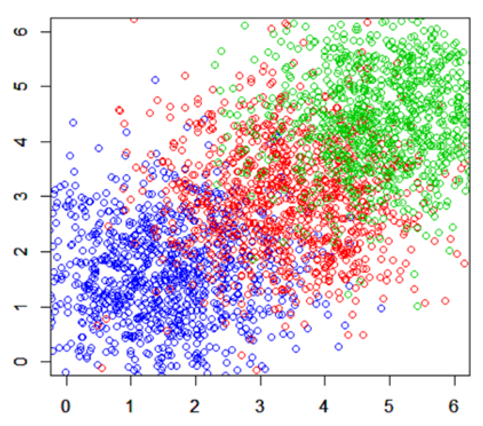
In this subsection, we used R software, version 4.3.0, to simulate and compute a mixture of three populations with mean vectors

$$\left\{\begin{array}{c}{\mathit{\mu }}_1=(1.5;1.5)\hfill \\ {\mathit{\mu }}_2=(3.5;3)\hfill \\ {\mathit{\mu }}_3=(5;4.5)\hfill \end{array}\right.,$$

(80)

and identical covariance matrices ${\mathit{I}}_2$. All measures were taken based on the corresponding normal homocedastic distributions. These values were assumed based on a reasonable assumption for the data generation process, taking into account the need for clear separation between the populations for effective simulation and analysis. In a real-world context, such as in the field of botany, these could, for example, represent averages of certain measurable traits, such as the lengths of petals from three different types of plants.

Simulated samples, with dimension 1000 were generated. These samples are presented in Figure 1.

Table 3. Costs of misallocation.

	${\mathit{P}}_1$	${\mathit{P}}_2$	${\mathit{P}}_3$
$P_1$	0	1	2
$P_2$	1	0	1
$P_3$	2	1	0

shows the costs of misallocation. The rows represent the real population of the elements and the columns the populations they were allocated to.

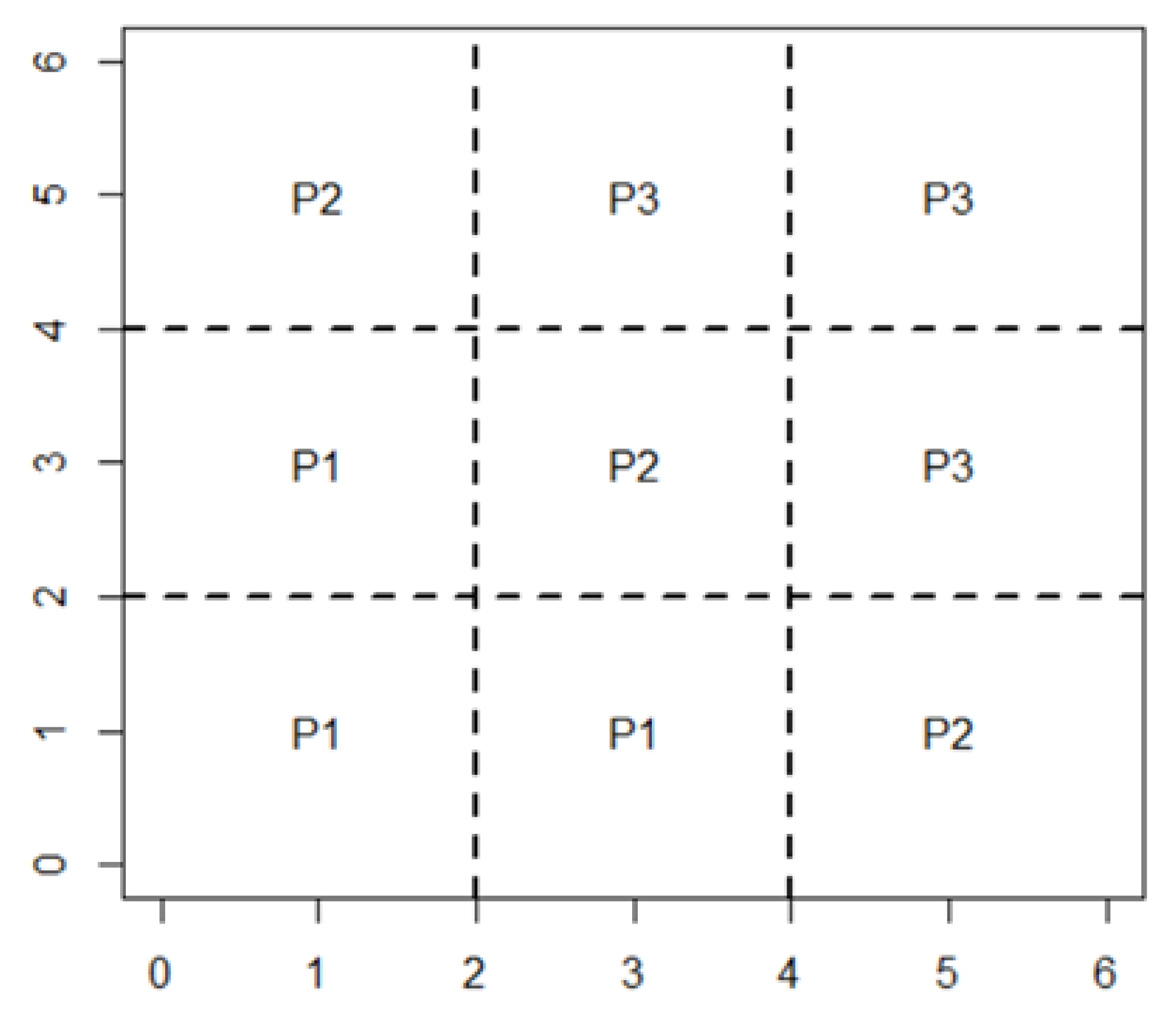
The shapes for the areas of distribution for the elements were established as illustrated in Figure 2. These are appropriate for normally distributed data with identical covariance matrices. The selected rectangular regions aligned with the axes allowed for efficient calculation of the probabilities of allocation and cost of misallocation.

The average cost will depend on the amount of elements that are allocated to $P_1$ from $P_2$ and to $P_2$ from $P_3$, as the probabilities of allocating to $P_3$ one element of $P_1$ and to $P_1$ one element of $P_3$ are very small.

With ${\mathcal{C}}_1$, ${\mathcal{C}}_2$ and ${\mathcal{C}}_3$ representing the regions in which the elements are allocated to populations $P_1$, $P_2$ and $P_3$, respectively, we must minimize

$$q={\int }_{{\mathcal{C}}_1}d{F}_2+{\int }_{{\mathcal{C}}_2}d{F}_1+{\int }_{{\mathcal{C}}_3}d{F}_2+{\int }_{{\mathcal{C}}_2}d{F}_3.$$

As shown in Figure 2, our approach was to optimize the points where the horizontal and vertical lines intersect the x-axis at $X=2$ and $X=4$ and the y-axis at $Y=2$ and $Y=4$, respectively. These intersection points act as delineations for the designated regions. The selection of those initial points was based on an informed estimation leveraging the mean vectors of the three populations. Noting the fact that the mean vectors for the three populations are ${\mu }_1=(1.5;1.5)$, ${\mu }_2=(3.5;3)$, and ${\mu }_3=(5;4.5)$, the initial points were chosen to lie approximately midway between these centroids. Taking into account that the populations are distributed normally with identical covariance matrices, this ensures that the initial delineations for the partitioning areas $({\mathcal{C}}_1,{\mathcal{C}}_2,{\mathcal{C}}_3)$ in the clustering process are not skewed towards one or more populations. Once these initial parameters were set, the optimization process was run, using the ‘stats’ package of R software, version 4.3.0. in R, particularly the ‘optim’ function, continually adjusting the parameters in order to find the values that minimized the objective function, which, in this case, was the cost of misallocation.

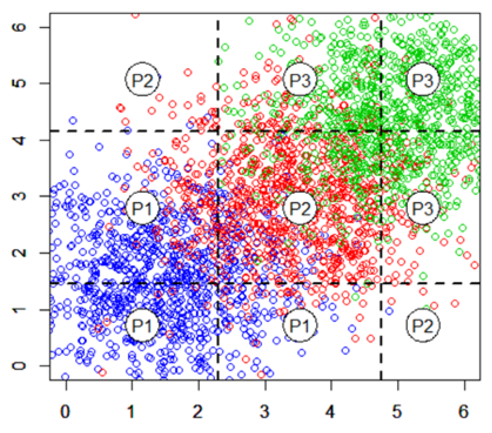
After 1000 repetitions of this optimization process, the suitable partitions displayed in Figure 3 were obtained. These partitions represent the areas of allocation for the elements within the three populations that produced the minimum misallocation cost, and, therefore, the most efficient allocation of elements within the identified clusters.

The cuts that are most cost-efficient can be represented by the straight lines

$$\left\{\begin{array}{cc}x=2.3;\hfill & x=4.75\hfill \\ y=1.45;\hfill & y=4.15\hfill \end{array}\right..$$

(81)

Table 4. Number of elements in each area.

$P_2$	$P_3$	$P_3$
$P_1=5$	$P_1=0$	$P_1=0$
$P_2=26$	$P_2=102$	$P_2=6$
$P_3=1$	$P_3=261$	$P_3=364$
$P_1$	$P_2$	$P_3$
$P_1=398$	$P_1=125$	$P_1=0$
$P_2=106$	$P_2=626$	$P_2=82$
$P_3=0$	$P_3=159$	$P_3=213$
$P_1$	$P_1$	$P_2$
$P_1=381$	$P_1=90$	$P_1=1$
$P_2=8$	$P_2=40$	$P_2=4$
$P_3=0$	$P_3=1$	$P_3=1$

shows the number of elements in each area.

The corresponding obtained total minimum cost was 638.

So, using simulated samples and different partitions of the sample, we were able to obtain the most cost-efficient cuts and the corresponding total minimum cost.

6. Conclusions

The paper discusses a comprehensive method to obtain optimal allocation rules for fixed-effect experiments. The study process is divided into four sections, namely, asymptotic distributions, confidence ellipsoids, inference, and optimal allocation rules.

Under the section of asymptotic distributions, the Central Limit Theorem (CLT) is accredited for providing valuable insights in terms of the behavior of sample averages.

In confidence ellipsoids, the ellipsoid properties are studied in developing a comprehensive understanding of the distribution of observations. The convex shape of the ellipsoid allows every point within the ellipsoid to be a convex combination of points on its boundary. Simultaneous confidence intervals can be constructed using these ellipsoids.

In the section on inference, the probability functions are detailed. These functions quantify the likelihood of obtaining specific results in experiments. As the number of trials increases, the asymptotic behavior of estimators is established. The distribution of estimated probabilities becomes approximately normal as the sample size grows.

The section on optimal allocation rules further elaborates on the methods for determining an allocation rule that minimizes the overall cost of assigning elements to their respective populations.

The paper concludes with two numerical applications. The first is a real data application showcasing the employment of computational techniques throughout the paper to analyze the real data. The second application undertakes the simulation of data to validate the findings of the study.