Article

Combining Autoregressive Integrated Moving Average Model and Gaussian Process Regression to Improve Stock Price Forecast

1
Guangxi Key Laboratory of Ocean Engineering Equipment and Technology, Beibu Gulf University, Qinzhou 535011, China
2
College of International Studies, Beibu Gulf University, Qinzhou 535011, China
*
Author to whom correspondence should be addressed.
Mathematics 2024, 12(8), 1187; https://doi.org/10.3390/math12081187
Submission received: 12 March 2024 / Revised: 9 April 2024 / Accepted: 12 April 2024 / Published: 15 April 2024
(This article belongs to the Special Issue Intelligence Optimization Algorithms and Applications)

Abstract

:
Stock market performance is one key indicator of the economic condition of a country, and stock price forecasting is important for investments and financial risk management. However, the inherent nonlinearity and complexity in stock price movements imply that simple conventional modeling techniques are not adequate for stock price forecasting. In this paper, we present a hybrid model (ARIMA + GPRC) which combines the autoregressive integrated moving average (ARIMA) model and Gaussian process regression (GPR) with a combined covariance function (GPRC). The proposed hybrid model can account for both the linearity and nonlinearity in stock price movements. Based on daily data on three stocks listed on the Shanghai Stock Exchange (SSE), it is found that GPRC outperforms GPR with a single covariance function. Further, the proposed hybrid model is compared with the ARIMA model, artificial neural network (ANN), and GPRC model. Based on the forecasting trend and the statistical performance of the four models, the ARIMA + GPRC model is found to be the dominant model for stock price forecasting and can significantly improve forecasting performance.

1. Introduction

Stock market performance is one key indicator of the economic condition of a country [1]. A stock market is a public and open market in which stocks and derivatives of a company are traded [2]. Stock prices fluctuate in the stock market because there are many factors influencing the stock market, such as general economic conditions, political events, and traders’ expectations [3]. Moreover, stock price movements are characterized by nonlinearities and high-frequent undulant components. Stock price forecasting is important for investors and stockbrokers. Thus, many researchers and financial analysts have tried to predict stock price trends with various techniques proposed over the years [4].
A time series model is often used to forecast stock prices. It is based on the past observations of the same variable, to build a model which can be used to predict the future trend. Note that it is not necessary to know the information of other variables in a time series model. One of the most efficient and widely used forecasting techniques for time series in social science is the autoregressive integrated moving average (ARIMA) model. The popularity of this model owes to its statistical properties and the famous Box–Jenkins methodology [5] in the modeling process. Recently, based on an analysis of three stock markets, Alshawarbeh and Abdulrahman [6] revealed that the hybrid ARIMA-ANN is overall superior to individual ANN and ARIMA models. Chen et al. [7] built an advanced hybrid model based on ARIMA to predict the prices of game stocks. ARIMA models are relatively more efficient and robust than complex structural models for short-run forecasting [8]. However, there is a major limitation for ARIMA, that is, the model presumes a linear correlation structure, and the nonlinear structure cannot be captured by the ARIMA model effectively. Thus, it is not satisfactory for many complex real-world problems. To circumvent this shortcoming and to model the nonlinear relationships observed in the real world, some nonlinear models such as the autoregressive conditional heteroscedastic (ARCH) model [9] and the threshold autoregressive (TAR) model [10] have been proposed. However, these nonlinear models only apply to some specific nonlinear relationships [11], and they may not work for other nonlinear structures of time series.
On the other hand, an artificial neural network (ANN) and support vector machine (SVM) are widely used in stock price forecasting because of their ability to capture the nonlinear characteristics in the data. Stock volatility represents a crucial impact in asset pricing models, portfolio management, and trading strategies. D’Ecclesia and Clementi [12] found that the artificial neural network (ANN) was the most accurate in tracking the implied stock volatility. Based on the characteristics of the same stock in different periods and the characteristics of different stocks in the same period, an adaptive SVR was presented by Guo et al. [13]. However, these methods still have some defects. They are good at capturing the nonlinear features in the data but may neglect some linear features.
In recent years, with the development of computer technology, deep learning has become a popular algorithm, which has been applied in image recognition, unmanned driving, and other fields. It is also applied in stock forecasting. Li et al. [14] proposed a clustering-enhanced deep learning framework to improve the accuracy of stock price prediction. Agrawal et al. [15] built an evolutionary deep learning model (EDLM), which is used to identify stock price trends. The model implements the deep learning model and establishes the concept of the related tensor. Although the deep learning algorithm shows good accuracy in stock price prediction, it has many internal parameters, and the process of adjusting parameters is complex and time-consuming.
Because of the non-stationary and chaotic characteristics of the stock price data [16], the time series data of stock prices may contain both linear and nonlinear features. Therefore, the combination of linear and nonlinear models can account for the complexity in modeling the stock market and overcome the limitation of individual technology [17]. Pai et al. [18] proposed a hybrid methodology based on the SVM model and ARIMA model to predict stock price. Based on the stock prices of 10 companies, it was found that the hybrid methodology performed better than the ARIMA model or the SVM model in predicting stock prices. Hajirahimi and Khashei proposed a new parallel hybrid model to implement an integrated hybrid framework in which all pure linear and nonlinear patterns in real time series can be appropriately simulated [19]. Li et al. [20] built some combined prediction models including ARIMA + SVM and ARIMA + ANN based on the artificial intelligence technique.
Adapting to the advantages and disadvantages of the algorithm or the characteristics of the data, a combined model can overcome the limitations of the single techniques and improve the prediction effect. Although some combination models have been applied in stock price forecasting, it is difficult to find an effective model with strong adaptability for the time series of stock prices with nonlinearity, interruption, and high-frequency fluctuation. Therefore, investors and financial institutions are keen to seek more effective forecasting models.
Gaussian process regression (GPR) is a highly valuable technique in the field of machine learning, and it is widely applied in many nonlinear problems [21,22,23,24] due to its advantages of being flexible, probabilistic, and nonparametric in the nonlinear modeling process. A GPR model is completely specified by the mean function and the covariance function. Therefore, compared to the neural network and support vector machines, the number of parameters for GPR is much less, and parameter optimization and convergence for GPR are easier. However, little research has been conducted on applying the Gaussian process regression algorithm in the field of stock market prediction.
In this paper, the ARIMA model which deals with linear characteristics and the GPR model which focuses on nonlinear characteristics are combined to form a new stock price forecasting model. It is expected that both linear and nonlinear characteristics of stock price movements can be captured by the proposed model, and better forecasting results can thus be obtained.
Specifically, the ARIMA model is first used to extract the linear features of the sample data for fitting and prediction. The residual sequence of the original data is obtained based on the fitting results. Then, the GPR model is used to train the residual sequence to obtain the nonlinear characteristics of the data. Finally, the results of the ARIMA model are modified and fine-tuned to improve the accuracy of forecasting, which is important for making investment decisions.
The rest of the paper is organized as follows. The stock price forecast model framework is developed in Section 2. The methodology is described in Section 3. Section 4 presents the results and analysis. Section 5 summarizes the paper with some concluding remarks.

2. Stock Price Forecast Model Framework

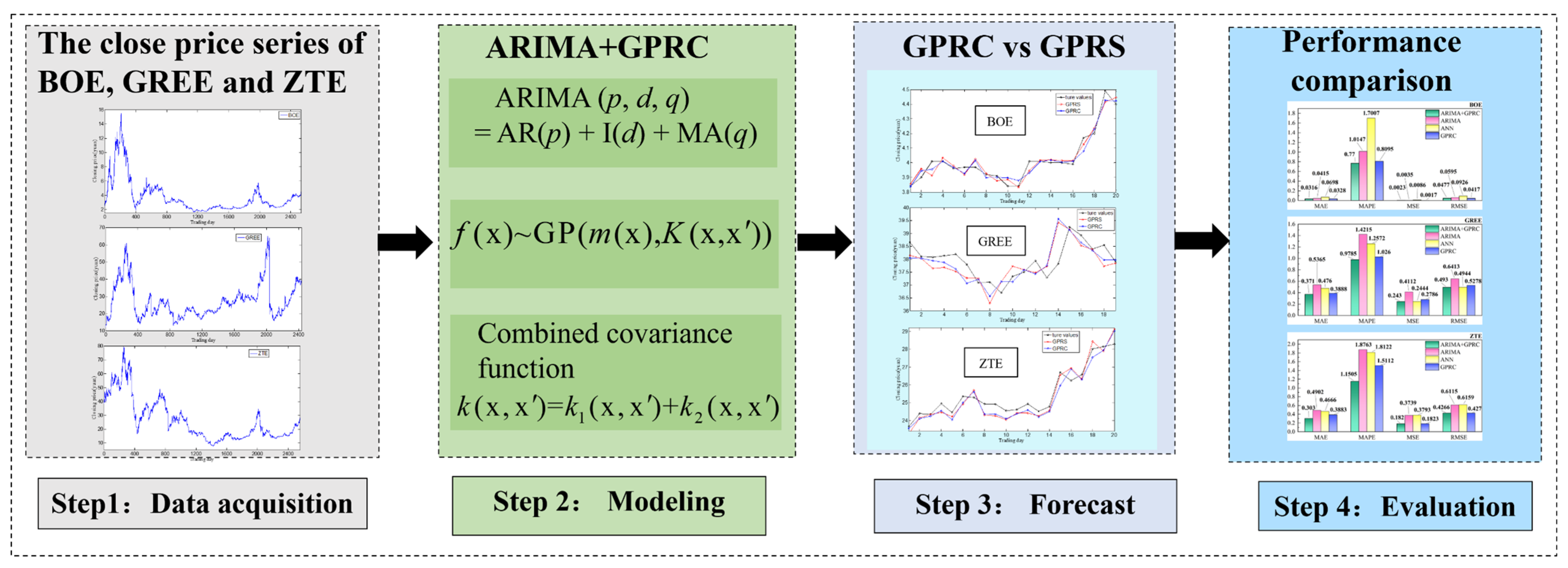
Figure 1 shows the framework of the stock price forecast model consisting of four steps.
In Figure 1, step 1 is data acquisition. This paper selects the closing prices of Beijing Oriental Electronics Technology Group Co., Ltd. (BOE) (Beijing, China), Gree Electric Appliances (GREE) (Zhuhai, China), and Zhongxing Telecommunication Equipment Corporation (ZTE) (Shenzhen, China) on the Shanghai Stock Exchange (SSE) (Shanghai, China) from 4 January 2007 to 30 September 2017, a total of 3923 trading days for the stock price forecast, of which 3893 trading days from 4 January 2007 to 31 August 2017 are the training set, and the remaining 30 trading days in September 2017 are the test set.
Step 2 is modeling. In order to solve the complex linear and nonlinear relationship between stock price time series, the ARIMA model can preliminarily estimate the range of autoregressive p and moving average q through the diagrams of the autocorrelation function (ACF) and partial autocorrelation function (PACF), which is suitable for capturing linear features. At the same time, two different covariance functions are combined to form a GPR model to focus on nonlinear characteristics, and then a mixed model of the ARIMA model and GPRC model is constructed for the stock price forecast.
Step 3 is the forecast. The forecast performance of the GPR model with a single covariance function (GPRS) and the GPR model with a combined covariance function (GPRC) are compared based on the three stocks.
Step 4 is evaluation. The mean absolute error (MAE), mean absolute percentage error (MAPE), mean square error (MSE), and root-mean-square error (RMSE) are common indicators of the forecast model. To verify the effectiveness of the proposed hybrid model, the mixed model (ARIMA + GPRC) is compared with the ARIMA, GPRC, and ANN models.

3. Methodology

3.1. ARIMA (p, d, q)

According to the autoregressive integrated moving average model ARIMA (p, d, q), the future value of a variable can be predicted by the past observations and random errors as follows [18,20]. The following introduction to the ARIMA model and related equations are all from Refs. [18,20].
y t = φ 1 y t 1 + φ 2 y t 2 + + φ p y t p + θ 0 + ε t θ 1 ε t 1 θ 2 ε t 2 θ q ε t q
where y t denotes the actual value, and ε t is the random error at time t; φ i ( i = 1 , 2 , , p ) and θ j ( j = 0 , 1 , 2 , , q ) are autoregressive coefficients and moving average coefficients, respectively. When q = 0, Equation (1) is an autoregressive (AR) model of order p. When p = 0, the model becomes a moving average (MA) model of order q.
Differencing and using logarithm are common ways to make the data become stable, and d is used to denote the time of differencing or logarithm. It is critical to determine the orders of the model, i.e., the p value and q value in ARIMA modeling. Usually, the determination of orders can be conducted by observing the correlation diagram of the autocorrelative function (ACF) and partial autocorrelation function (PACF). However, it is not accurate to determine the orders only through the trail and truncation of the ACF and PACF. Akaike Information Criterion (AIC) and Bayesian Information Criterion (BIC) can be used to further determine the values of p and q.
AIC ( p ) = n ln σ ε 2 + 2 p
BIC ( p ) = n ln σ ε 2 + p ln n
where n denotes the number of observations, and p is the number of parameters which are to be estimated, i.e., the order of autoregression. σ ε 2 = t = 1 n ε t 2 represents the sum of squared residuals. In (2) and (3), ln σ ε 2 decreases as p increases, while 2p and p ln n increase as p increases. Thus, the p value is considered to be an appropriate order of the model when AIC(p) or BIC(p) is minimalized. AIC(p) and BIC(p) are applied for small and large sample data, respectively. When the orders are specified, the estimation of the model parameters is straight-forward and can be conducted by the least square method.

3.2. The GPR Model Based on a Single and Combined Covariance Function

It is well known that the Gaussian process (GP) model has the advantages of a flexible modeling ability and high approximation accuracy for nonlinear problems, compared to other classes of nonlinear models. In particular, the GP model can approximate a function with high accuracy when the sample data are small. The usage and modeling properties of the Gaussian process were reviewed by Rasmussen et al. [25]. The following introduction to the GPR model and related equations are all from Ref. [25] A Gaussian process is completely specified by its mean function m(x) and covariance function K ( x , x ) ; it can be represented as f ( x ) G P ( m ( x ) , K ( x , x ) ) , where x , x R d are arbitrary random variables.
For the training set D = { ( x i , y i } | i = 1 , 2 , , n } , observation value Y = ( y 1 , y 2 , , y i ) T , the prior distribution of Y and the joint prior distribution between Y and the forecast valued of the test point y * are obtained as follows.
Y N ( 0 , K ( X , X ) + σ n 2 I n )
[ Y y * ] N ( 0 , [ K ( X , X ) + σ n 2 I n K ( X , x * ) K ( x * , X ) K ( x * , x * ) ] )
where I n denotes an n-dimensional identity matrix, and X is the training set data; x * is defined as test point data; K ( X , X ) is the n-th covariance matrix of X . K ( X , x * ) represents the covariance matrix of X , and x * , K ( x * , x * ) is the x * covariance matrix.
The covariance function is a key part in the GP model. The similarity of data points is very important in supervised learning. For example, if points a and b are similar, the corresponding function values f(a) and f(b) will also be similar. The covariance function is defined as the distance between the output variables corresponding to two random input variables and is used to measure the similarity of data points. There are many kinds of covariance functions in the GP model, and it is not easy to choose the most suitable one. The squared exponential covariance function is most frequently used, and it is given as
K 1 ( x , x ) = σ f 2 exp ( ( x x ) 2 2 l 2 ) + σ n 2 δ ( x , x )
where σ f 2 represents the overall measurement of prior knowledge; l f is a correlation measurement hyperparameter. δ ( x , x ) is the Kronecker operator, whose value when two data are the same is 1, otherwise its value is 0.
However, a single covariance function only captures a single feature. In order to describe different characteristics of the data and enhance the nonlinear mapping capability of the covariance function, this paper combines the squared exponential covariance function with the linear covariance function to capture the smooth and secular trend, respectively. The expression of the exponential covariance function is shown in Equation (5).
K 2 ( x , x ) = x x
The combined covariance function is
K ( x ,   x ) = K 1 ( x ,   x ) + K 2 ( x ,   x )
Note that the sum of two kernels is still a kernel [25]. All the hyperparameters in the GP model with the combined covariance function can be denoted as Equation (7).
θ = { l , σ n , σ f }
After determining the type of covariance function, the calculation of hyperparameters θ is a crucial step in determining the GPR model. The marginal likelihood of the GPR model provides an effective method for directly solving hyperparameters using the training set, which is an advantage of GPR.
The process of solving hyperparameters is as follows: first, determine the likelihood function L ( θ ) as the negative logarithm of the conditional probability of the training set, and obtain the partial derivative of the hyperparameter. Then, using the conjugate gradient method to solve the hyperparameters when the likelihood function reaches its minimum value, the obtained hyperparameters are the optimal hyperparameters. The partial derivatives of the likelihood function are shown in Equation (8) [25].
L ( θ ) = 1 2 Y T K ( X , X ) + σ n 2 I n ) 1 Y + 1 2 lg | K ( X , X ) + σ n 2 I n | + π 2 lg 2 π
According to the Bayesian posterior probability formula, the posterior distribution of the forecast value y * of the test point is y * | X , Y , x * N ( μ y * , σ y * 2 ) , and the mean μ y * is taken as the predicted forecast at x * , where the mean μ y * and variance σ y * 2 are represented by Equations (9) and (10), respectively.
μ y * = K ( x * , X ) [ K ( X , X ) + σ n 2 I n ) 1 y *
σ y * 2 = K ( x * , x * ) K T ( x * , X ) [ K ( X , X ) + σ n 2 I n ) 1 K ( x * , X )

3.3. Combining Model of ARIMA and GPR (ARIMA+GPR)

The stock price time series is impacted by many factors, and it may not be simply linear or nonlinear. Thus, stock price forecasting is a complex problem. It may be inadequate to approximate the stock price time series by ARIMA models due to the assumption of the linear structure. Moreover, using GPR to handle linear and nonlinear relationships in the same time series may yield mixed results, although GPR has good nonlinear adaptability [25]. Therefore, a hybrid methodology based on ARIMA models and GPR is proposed for stock forecasting in this paper. It can account for both the linear and nonlinear modeling capabilities. When a time series has a linear autocorrelation structure and a nonlinear component, the combining methodology can be effective. The forecast of the combined methodology is as follows:
y ^ t = L ^ t + N ^ t
where L ^ t and N ^ t denote the estimated value of the linear component and nonlinear component, respectively, at time t.
The implementation of the hybrid methodology consists of three steps. First, use ARIMA to model sample data, and obtain the forecast value L ^ t at time t. Second, calculate the deviation between the forecast value L ^ t of the ARIMA model and the actual value y t , i.e.,
ε t = y t L ^ t
Third, in order to indicate the nonlinear relationships, GPR is used to model residuals which come from the ARIMA model. The GPR model for the residuals is as follows:
ε ^ t = f ( ε t 1 , ε t 2 , , ε t r ) + Δ t
where r is the larger value between the autoregressive parameter (p) and moving average parameter (q) of the ARIMA model, Δ t expresses the random error, and f denotes the nonlinear function determined by GPR. So ε ^ t represents the forecasting value of the nonlinear component at time t, namely N ^ t from Equation (11).

4. Results and Analysis

The Shanghai Stock Exchange (SSE) is one of the two stock exchanges in Mainland China, and it is one of the largest stock markets in the world. More and more investors from both China and abroad are attracted to the SSE for the potential to gain high returns. Thus, it is important to understand the stock price movements in the SSE, and stock price forecasting has been an important research topic. In this paper, we therefore use published stock price data from the SSE.
MATLAB R2018a software is used for testing and validation. The proposed hybrid GPR model and GPR model is implemented with the help of the GPML (Gaussian processes for machine learning) toolbox. The neural network toolbox in MATLAB R2018a is adopted for building the ANN model.

4.1. Data Set and Evaluating Indicators

In this paper, we use the historical daily close prices from the SSE, as the close prices reflect all the trading activities of the day. Three companies listed on the SSE are selected: BOE, GREE, and ZTE for this study. The sample period is from 4 January 2007 to 30 September 2017.
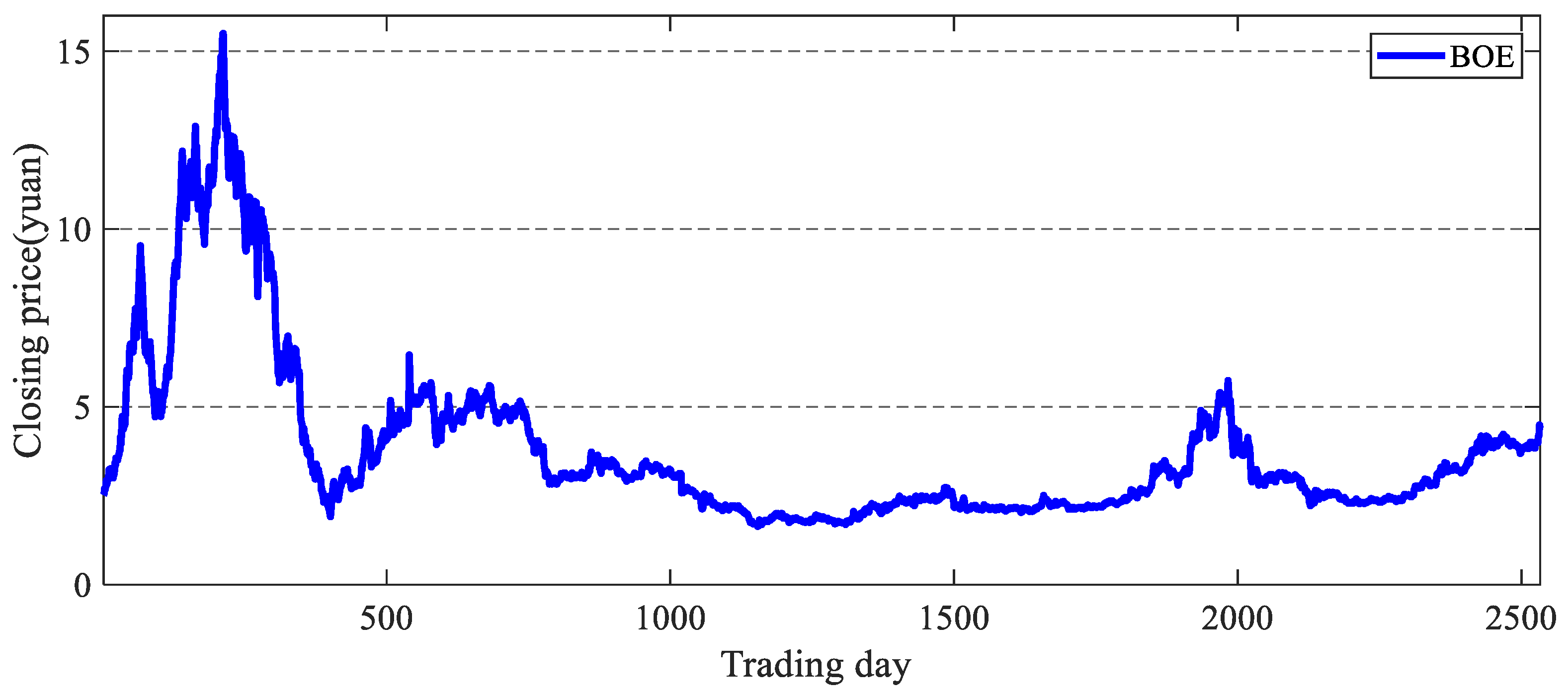
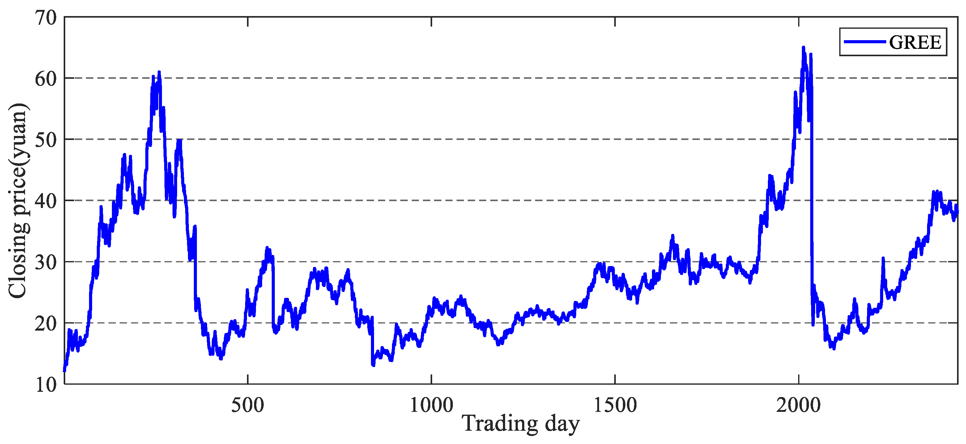
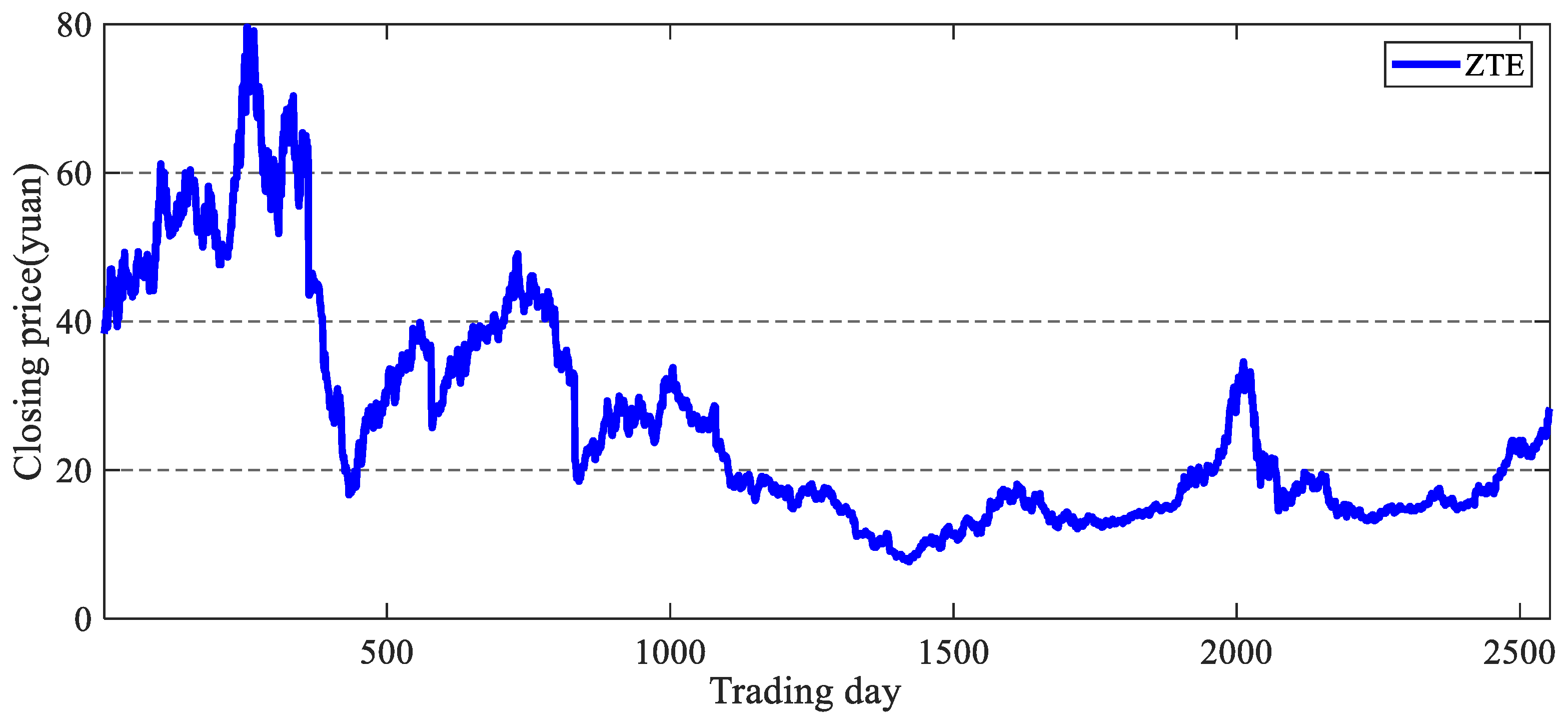
Figure 2, Figure 3 and Figure 4 display the time series of the closing prices for BOE, GREE, and ZTE, respectively. Each data set is partitioned into two parts: the data from 4 January 2007 to 31 August 2017, for training and the remaining samples (September 2017) for testing. The training data set is used to build the forecasting models, and the effectiveness of the forecasting models is assessed based on the test data set. Table 1 shows the detailed information of the training and testing data set.
To evaluate the performance of the hybrid model quantitatively, four performance indicators which measure the deviation between the predicted and the observed values are selected: the mean absolute error (MAE), mean absolute percentage error (MAPE), mean square error (MSE), and root-mean-square error (RMSE). Smaller values of these measures usually indicate better predictive performance. They are given as
MAE = 1 n i = 1 n | y i y ^ i |
MAPE = 1 n i = 1 n ( | y i y ^ i | / y i 100 % )
MSE = 1 n i = 1 n | y i y ^ i | 2
RMSE = 1 n i = 1 n | y i y ^ i | 2
where y i and y ^ i are the observed and predicted stock price at time i, respectively; n denotes the number of predicted data.

4.2. Comparison of GPR Model with Single vs. Combined Covariance Function

In order to select the more appropriate covariance function of the GPR model, we compare the forecasting performance of the GPR model with a single covariance function (GPRS) and that of the GPR model with a combined covariance function (GPRC). Figure 5, Figure 6 and 
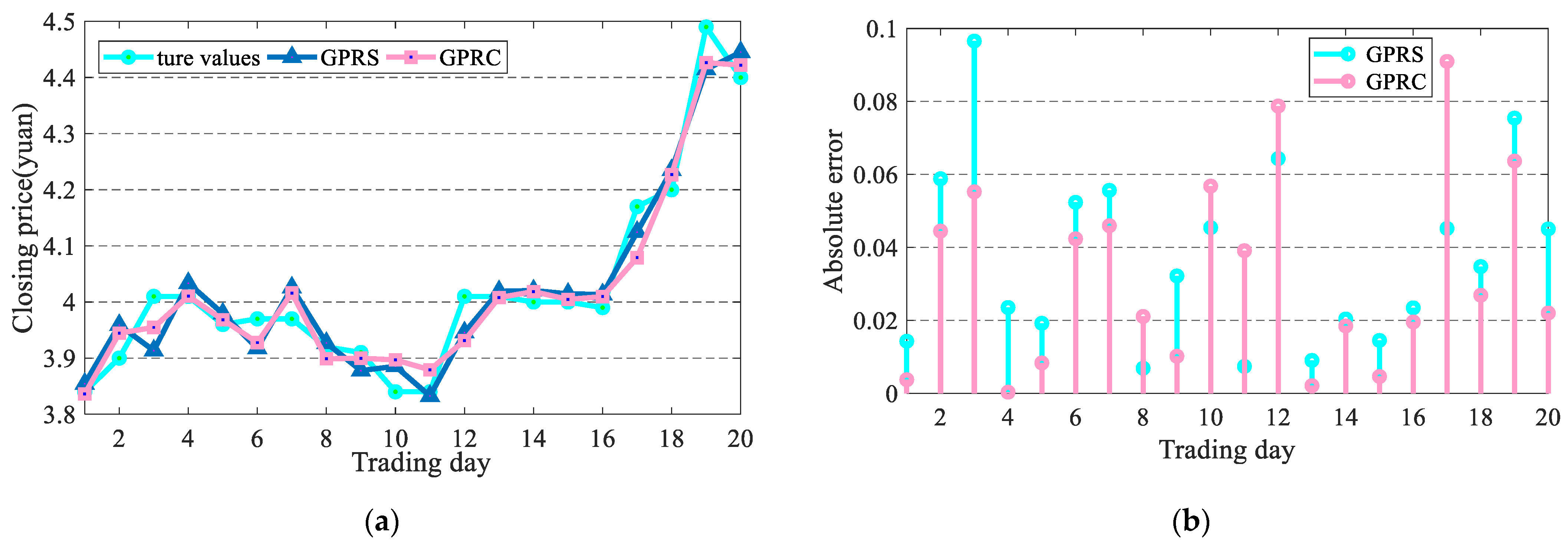
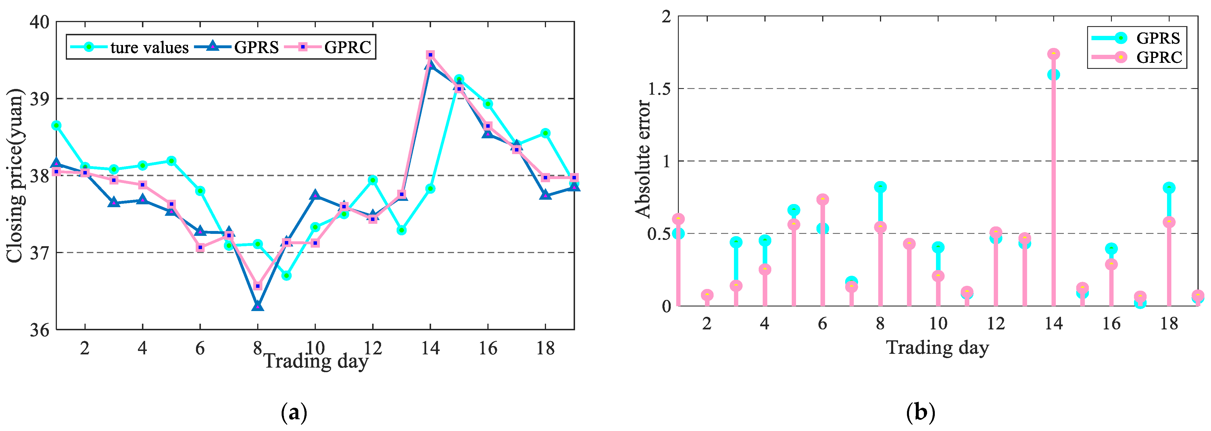
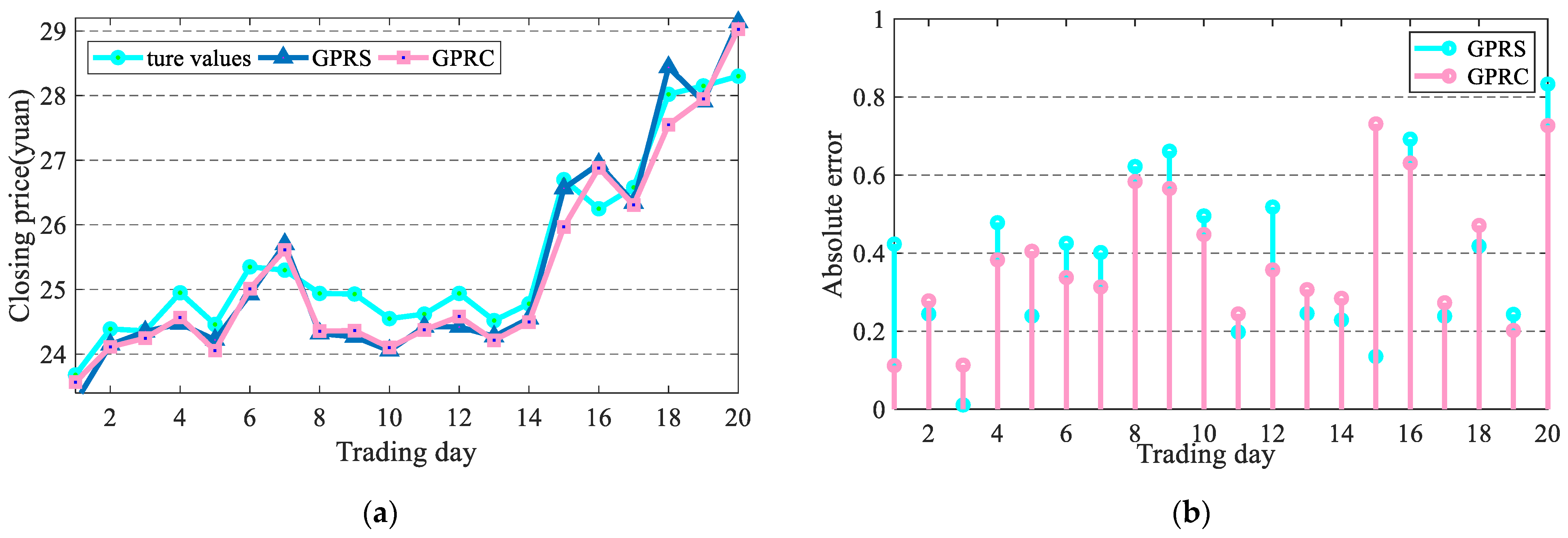
Figure 7 show the forecast results by a single and combined covariance function (GPRS and GPRC models) for the three selected stocks. From Figure 5a, Figure 6a and Figure 7a, it can be seen that both GPRC and GPRS can obtain curves with similar trends to the actual curve, but the predicted curve obtained by GPRC is closer to the actual curve than GPRS. In Figure 5b, the absolute errors obtained by GPRS and GPRC are both very small, with the maximum absolute error not exceeding 0.1. Among the 20 testing samples, 15 of the absolute error values obtained by GPRC are less than those of GPRS. Figure 6b shows the absolute error of GPRS and GPRC in obtaining the test set. Except for the error value greater than 1 in the 14th test sample, all others are less than 1. Although the error value of 11 samples obtained by GPRC is greater than that of GPRS, 8 of them are only slightly greater than that of GPRS. In Figure 7b, the absolute errors obtained by GPRS and GPRC are also very small, and the maximum absolute error does not exceed 0.1, and for the 20 samples tested, 14 of the absolute error values obtained by GPRC are less than GPRS. Therefore, it is clear from Figure 5, Figure 6 and Figure 7 that the forecasting accuracy of GPRC is higher than that of GPRS. Table 2, Table 3 and Table 4 present the evaluation indicators of the forecasting performance. In Table 2, Table 3 and Table 4, for BOE and GREE, all indicators of GPRC are smaller than those for GPRS. For ZTE, the same holds for all indicators except MAE. Overall, the forecasting accuracy of the GPRC model is better than that of the GPRS model.

4.3. Forecasting Results of Various Models and Comparative Analysis

In order to validate the forecasting accuracy of the proposed model, we compare it with a few other models including ARIMA, GPRC, and an ANN. As shown above, the GPRC model outperforms GPRS; GPRS is not considered in this section.
For the ANN model, we employ a three-layer (one of which is a hidden layer) perceptron model, because it can approximate any continuous function in a reasonable way [26]. The number of hidden nodes is the integer number closest to log(n), where n is the number of training observations [26]. Five input variables are grouped into one vector as the input for day t − 1. These variables are the daily high price (Ht−1), daily low price (Lt−1), the open price (Ot−1), daily close price (Ct−1), and trading volume (Vt−1). The output variable is the close price for day t. For the GPRC model, the input and output variables are the same as those for the ANN model. Figure 8, Figure 9 and Figure 10 show the forecast values and absolute errors across different models (ARIMA, GPRC, ANN, ARIMA + GPRC) for the three selected stocks, respectively, and the evaluation indicator values of the four models are shown in Figure 11, Figure 12 and Figure 13.
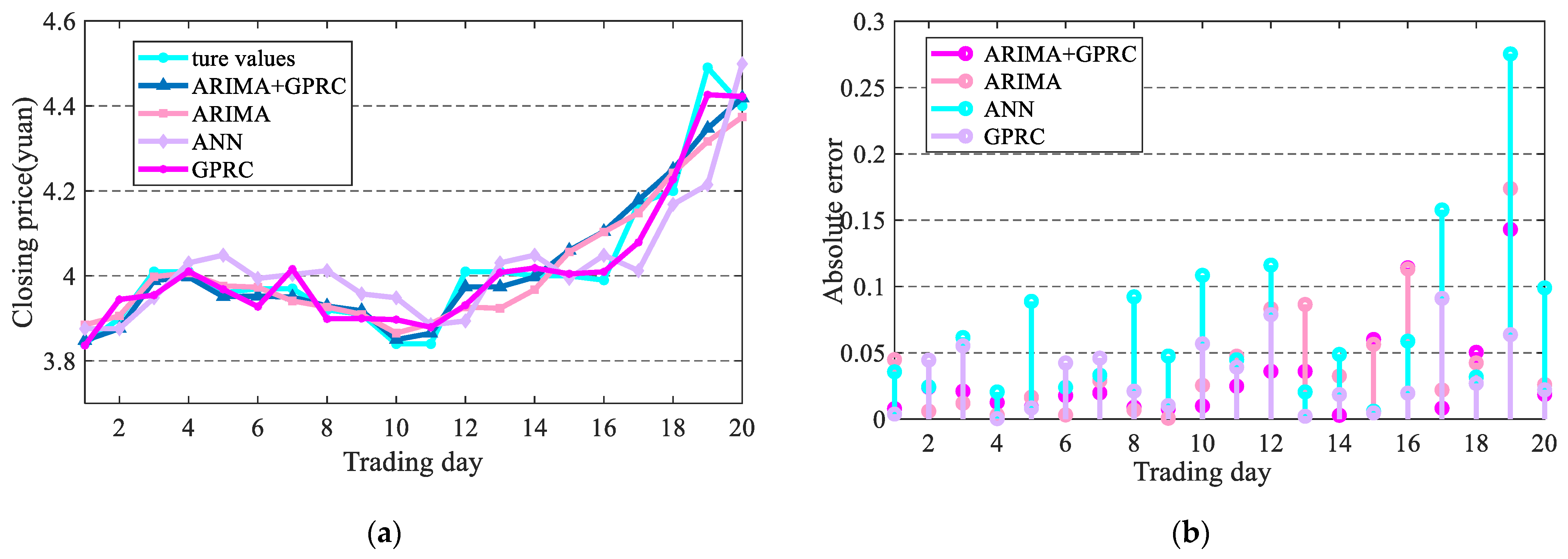
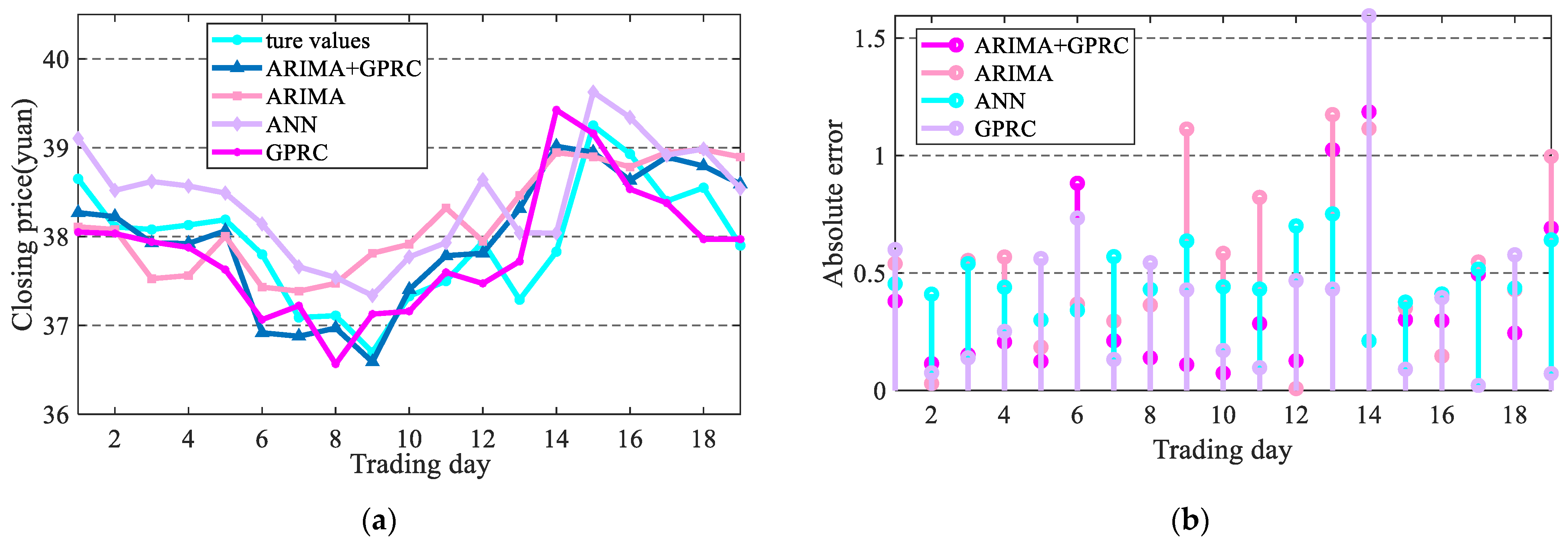
The forecasting curves and the absolute errors of four forecasting models on BOE are shown in Figure 8. In Figure 8a, all four models can obtain the same trend as the actual curve, and overall, the ARIMA + GPRC curve is closer to the actual curve. In 
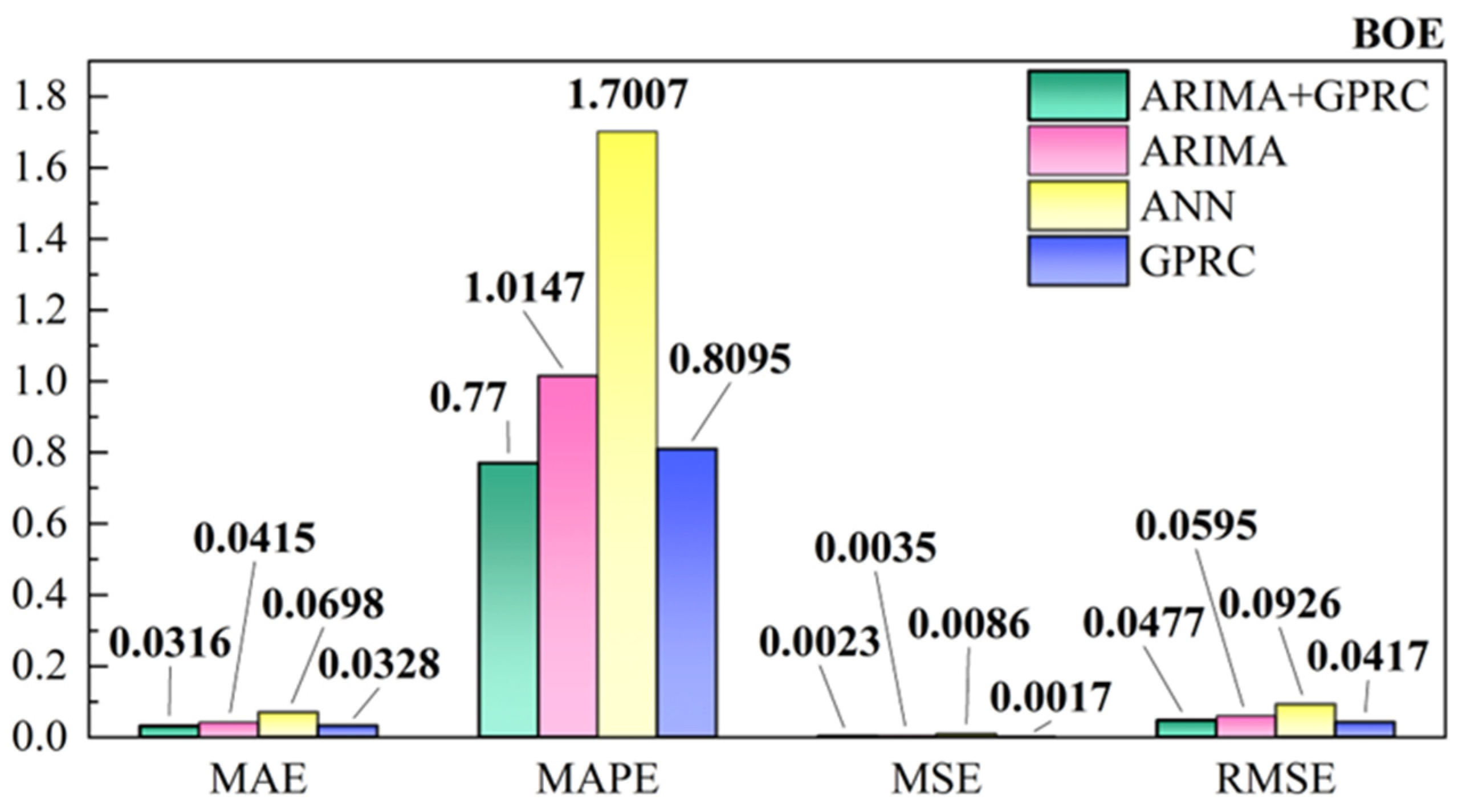
Figure 8b, the absolute error obtained by the four models is very small, with a maximum error of no more than 0.3. Among the 20 test samples, ARIMA + GPRC has 7 samples with less error than the other three models, ARIMA has 4 samples with less error than the other three models, and GPRC has 8 samples with less error than the other three models. A further analysis of the evaluation indicators in Figure 11 shows that among the evaluation indicators obtained by ARIMA + GPRC except for REMS slightly greater than GPRC, all other indicators are smaller than models ARIMA, ANN, and GPRC. Therefore, for the closing price forecast of BOE, the ARIMA + GPRC forecasting accuracy constructed is better than the three models compared.
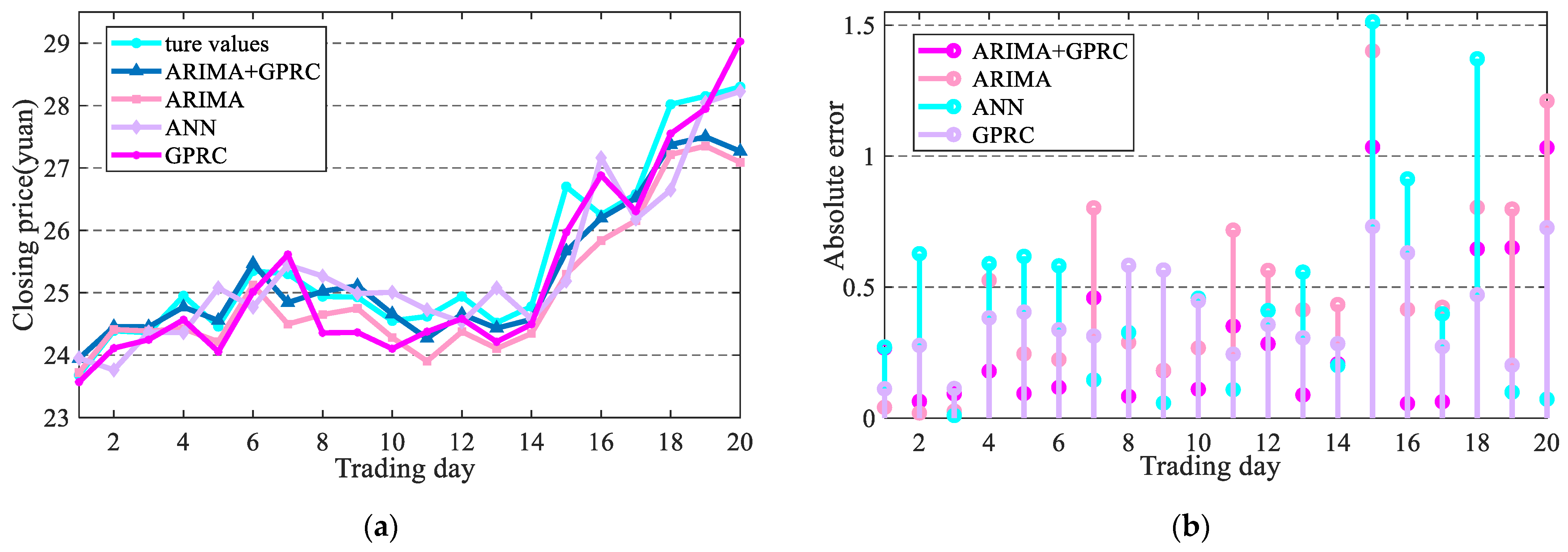
In Figure 9a, four models can obtain the same trend as the actual curve of the closing price forecast for GREE; the forecasting curves of the first 12 samples obtained by ARIMA + GPRC are the closest to the actual curves among the four models. In Figure 9b, the absolute error obtained by the four models is small; except for samples 16, 19, and 20, the absolute errors of all samples are less than 1. Among the 19 test samples, ARIMA + GPRC has 7 samples with less error than the other three models, ARIMA has 3 samples with less error than the other three models, and GPRC has 7 samples with less error than the other three models. In 
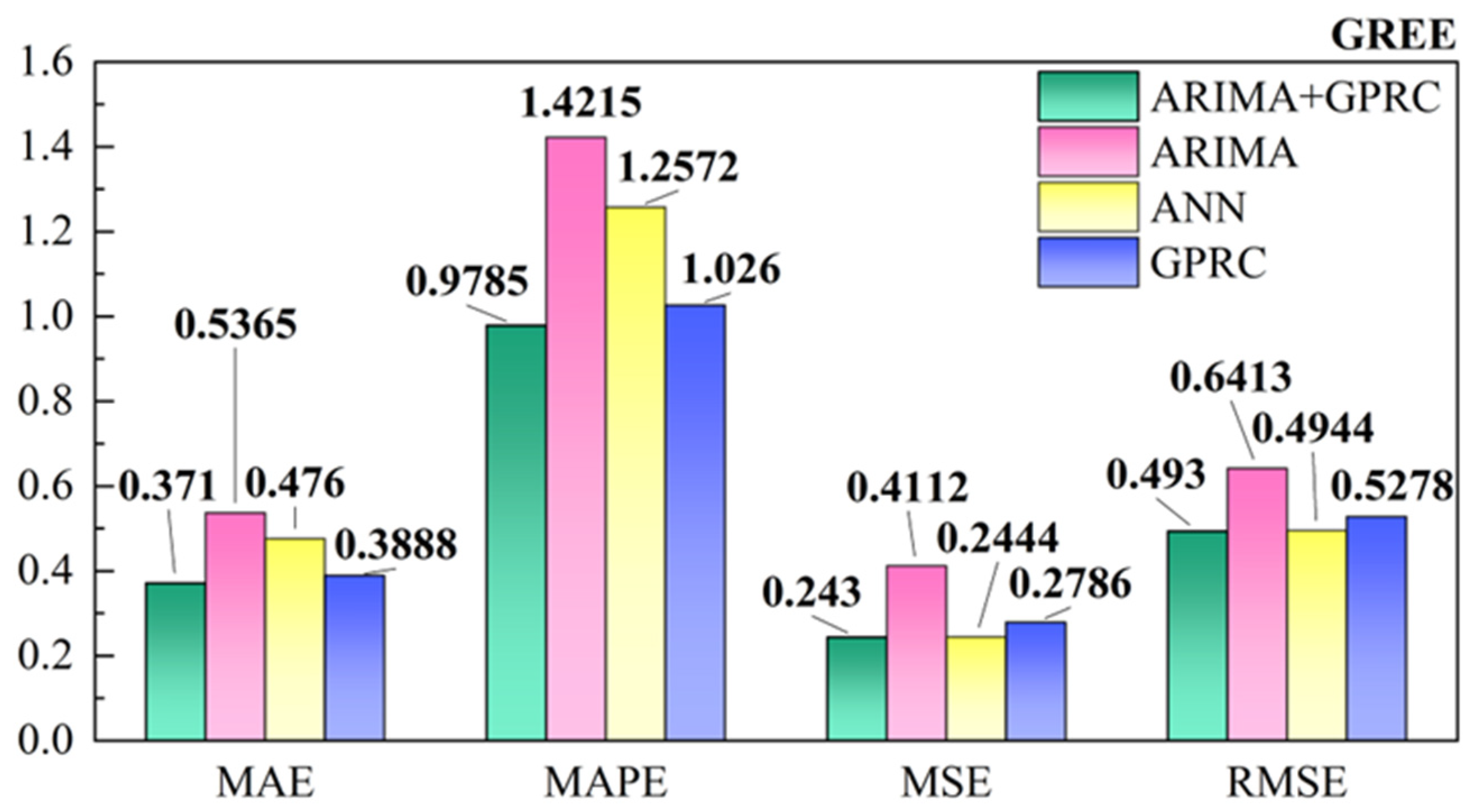
Figure 11, all evaluation indicators obtained by ARIMA + GPRC are smaller than the other three models. Therefore, for the closing price forecast of GREE, the ARIMA + GPRC constructed is superior to the three models compared.
From 
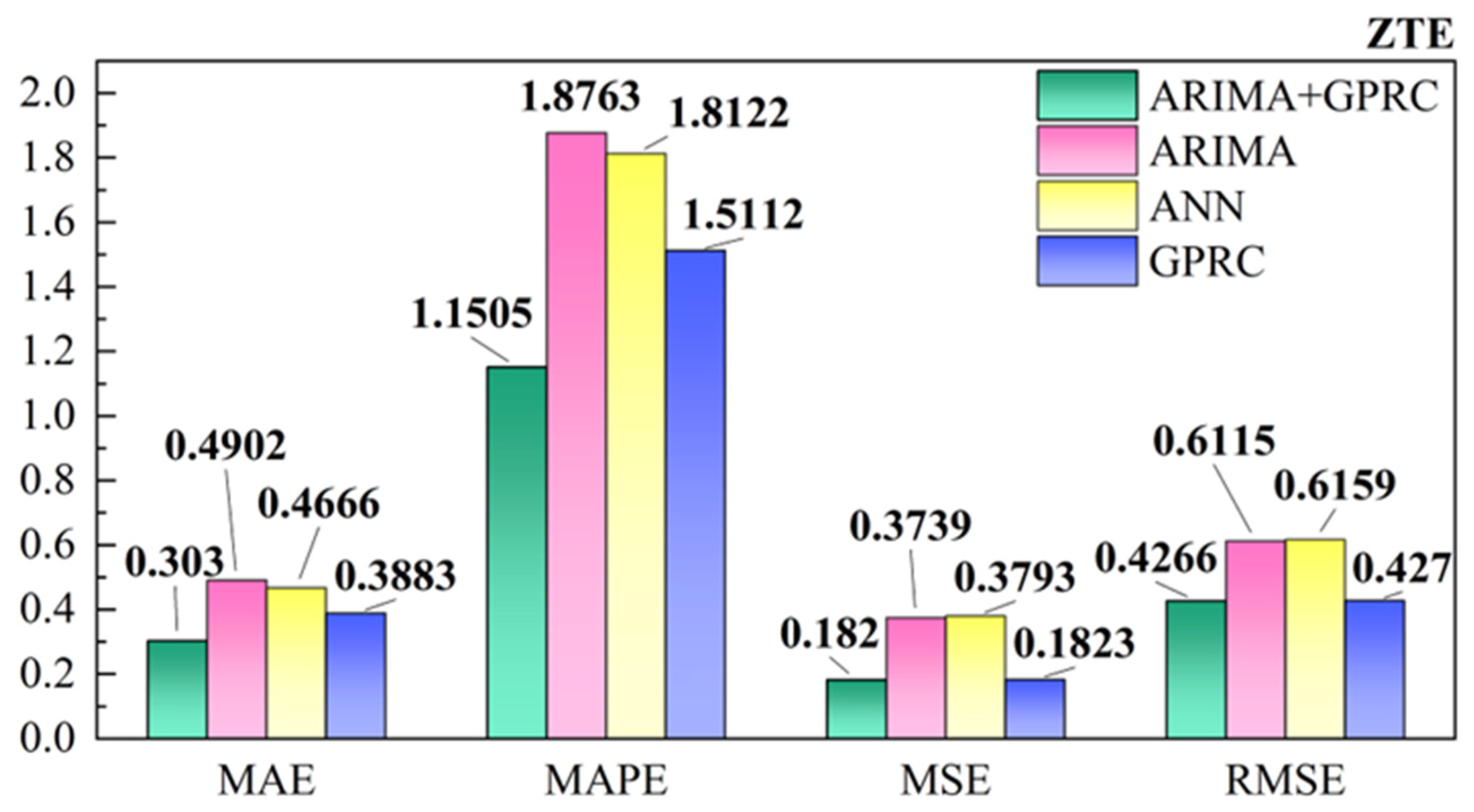
Figure 10a, it can be seen that all four models can obtain trends similar to the actual curve, except for samples 15, 19, and 20, ARIMA + GPRC can obtain the curve closest to the actual curve. In Figure 10b, the absolute error obtained by the four models is very small; except for samples 16, 18, and 20, the absolute errors of all samples are lower than 1. And among the test samples, ARIMA + GPRC, ARIMA, GPRC, and ANN have nine, two, two, and seven samples with less error than the other three models, respectively. And it is clear from Figure 13 that the ARIMA + GPRC model obtains the smallest value of all evaluation indicators among the four models. For the closing price of BOE, the MAPE obtained by ARIMA + GPRC increased by 24.1%, 54.7%, and 4.9%, respectively, by comparing to the ARIMA, ANN, and GPRC models. Calculating the forecast indicators for the GREE closing price, it was found that the MAPE of ARIMA + GPRC jumped by 31.2%, 22.2%, and 4.6%, respectively, by comparing to the models ARIMA, ANN, and GPRC. And analyzing the accuracy of the ZTE closing prices forecasted by four models, comparing to the ARIMA, ANN, and GPRC models, the MAPE for the ARIMA + GPRC model also increased by 38.7%, 36.5%, and 23.9%, respectively. Therefore, the ARIMA + GPRC model has best the forecasting accuracy among the four models.
It can be seen from Figure 8, Figure 9, Figure 10, Figure 11, Figure 12 and Figure 13 that the mixture model (ARIMA + GPRC) developed in this paper has excellent forecasting accuracy, which verifies the effectiveness and feasibility of the model built.

5. Conclusions

Over the years, a lot of research has been devoted to stock price forecasting which is critical for investment decisions. However, there are hardly any effective forecasting models. Thus, it is necessary to continue to study how to improve the effectiveness of forecasting models. In addition, it is usually difficult to predict stock prices accurately due to the complexity and volatility of the stock market.
This paper presents a new hybrid model which combines ARIMA with GPR, to improve the forecasting performance of the stock market in terms of statistical and financial terms. Meanwhile, in order to select more suitable covariance functions, the GPR model with different types of covariance functions is evaluated. It is found that GPR with a combined covariance function outperforms GPR with a single covariance function. Based on the proposed hybrid model, the ARIMA model captures the linear structure of stock prices series, and the nonlinear structure is modeled by GPRC. And using three actual data sets of the trading day price verified the validity of the ARIMA + GPRC model. The simulation results indicated that compared with ARIMA, ANN, and GPRC, in most cases, the proposed hybrid model gave the best forecasting performance in terms of MAE, MAPE, MSE, and RMSE. In summary, it can be concluded that the proposed method is an effective way to improve forecasting performance, which is beneficial to investors for investment decisions and risk management.
There are many factors that affect stock prices; in this study, only the influence of historical closing prices was considered; other influencing factors on the stock market will be taken into account in future research, which contributes to uncovering their functions and subsequent deep penetration into this area.

Author Contributions

Methodology, S.T., H.M. and J.L.; formal analysis, S.T. and Y.L.; investigation, J.H. and H.M.; writing—original draft, S.T. and Y.L.; supervision, Y.L.; funding acquisition, J.L. All authors have read and agreed to the published version of the manuscript.

Funding

This research was supported by the National Natural Science Foundation of China (NSFC) (Grant No. 52365059), the Natural Science Foundation of Guangxi (Grant Nos. 2020JJD160004 and 2019JJB160048) and Beibu Gulf University Scientifc Research Initiation Project of Introducing High level Talents (Grant No.2022KYQD13).

Data Availability Statement

The data used to support the findings of this study are available from the corresponding author upon request.

Conflicts of Interest

The authors declare that there are no conflicts of interest regarding the publication of this paper. All authors have no conflicts of interest. This article does not contain any studies with human participants performed by any of the authors.

References

  1. Mohan, M.; Raja, P.K.; Velmurugan, P.; Kulothungan, A. Holt-winters algorithm to predict the stock value using recurrent neural network. Methods 2023, 8, 10. [Google Scholar] [CrossRef]
  2. Buche, A.; Chandak, M.B. Stock market forecasting techniques: A survey. J. Eng. Appl. Sci. 2019, 14, 1649–1655. [Google Scholar] [CrossRef]
  3. Hadavandi, E.; Shavandi, H.; Ghanbari, A. Integration of genetic fuzzy systems and artificial neural networks for stock price forecasting. Knowl.-Based Syst. 2010, 23, 800–808. [Google Scholar] [CrossRef]
  4. Zhao, C.; Hu, P.; Liu, X.; Lan, X.; Zhang, H. Stock market analysis using time series relational models for stock price prediction. Mathematics 2023, 11, 1130. [Google Scholar] [CrossRef]
  5. Box, G.E.; Jenkins, G.M.; Reinsel, G.C.; Ljung, G.M. Time Series Analysis: Forecasting and Control; John Wiley & Sons: Hoboken, NJ, USA, 2015. [Google Scholar]
  6. Alshawarbeh, E.; Abdulrahman, A.T.; Hussam, E. Statistical Modeling of High Frequency Datasets Using the ARIMA-ANN Hybrid. Mathematics 2023, 11, 4594. [Google Scholar] [CrossRef]
  7. Chen, Y.S.; Chou, C.L.; Lee, Y.J.; Chen, S.F.; Hsiao, W.J. Identifying Stock Prices Using an Advanced Hybrid ARIMA-Based Model: A Case of Games Catalogs. Axioms 2022, 11, 499. [Google Scholar] [CrossRef]
  8. Meyler, A.; Kenny, G.; Quinn, T. Forecasting Irish Inflation Using ARIMA Models; MPRA: Munich, Germany, 1998. [Google Scholar]
  9. Engle, R.F. Autoregressive conditional heteroscedasticity with estimates of the variance of United Kingdom inflation. Econom. J. Econom. Soc. 1982, 50, 987–1007. [Google Scholar] [CrossRef]
  10. Tong, H. Threshold Models in Non-Linear Time Series Analysis; Springer Science & Business Media: Berlin/Heidelberg, Germany, 2012. [Google Scholar]
  11. De Gooijer, J.G.; Kumar, K. Some recent developments in non-linear time series modelling, testing, and forecasting. Int. J. Forecast. 1992, 8, 135–156. [Google Scholar] [CrossRef]
  12. D’Ecclesia, R.L.; Clementi, D. Volatility in the stock market: ANN versus parametric models. Ann. Oper. Res. 2021, 299, 1101–1127. [Google Scholar] [CrossRef]
  13. Guo, Y.; Han, S.; Shen, C.; Li, Y.; Yin, X.; Bai, Y. An adaptive SVR for high-frequency stock price forecasting. IEEE Access 2018, 6, 11397–11404. [Google Scholar] [CrossRef]
  14. Li, M.; Zhu, Y.; Shen, Y.; Angelova, M. Clustering-enhanced stock price prediction using deep learning. World Wide Web 2022, 26, 207–232. [Google Scholar] [CrossRef] [PubMed]
  15. Agrawal, M.; Shukla, P.K.; Nair, R.; Nayyar, A.; Masud, M. Stock prediction based on technical indicators using deep learning model. Comput. Mater. Contin. 2022, 70, 287–304. [Google Scholar] [CrossRef]
  16. Hall, J.W. Adaptive Selection of US Stocks with Neural Nets. In Trading on the Edge: Neural, Genetic, and Fuzzy Systems for Chaotic Financial Markets; Wiley: New York, NY, USA, 1994; pp. 45–65. [Google Scholar]
  17. Bahrammirzaee, A. A comparative survey of artificial intelligence applications in finance: Artificial neural networks, expert system and hybrid intelligent systems. Neural Comput. Appl. 2010, 19, 1165–1195. [Google Scholar] [CrossRef]
  18. Pai, P.F.; Lin, C.S. A hybrid ARIMA and support vector machines model in stock price forecasting. Omega 2005, 33, 497–505. [Google Scholar] [CrossRef]
  19. Hajirahimi, Z.; Khashei, M. A novel parallel hybrid model based on series hybrid models of ARIMA and ANN models. Neural Process. Lett. 2022, 54, 2319–2337. [Google Scholar] [CrossRef]
  20. Li, Y.; Wu, C.; Liu, J.; Luo, P. A combination prediction model of stock composite index based on artificial intelligent methods and multi-agent simulation. Int. J. Comput. Intell. Syst. 2014, 7, 853–864. [Google Scholar] [CrossRef]
  21. Li, X.; Zhang, Y.; Li, D.; Shum, P.P.; Huang, T. Nonlinear channel equalization using Gaussian Processes Regression in IMDD fiber link. IEEE Photonics J. 2022, 14, 1–6. [Google Scholar] [CrossRef]
  22. Zheng, Y.; Zhang, W.; Liu, T.; Zhang, Y.F. Resonant responses and double-parameter multi-pulse chaotic vibrations of graphene platelets reinforced functionally graded rotating composite blade. Chaos Solitons Fractals 2022, 156, 28. [Google Scholar] [CrossRef]
  23. Zheng, J.; Gong, Y.; Liu, W.; Zhou, L. Subspace Gaussian process regression model for ensemble nonlinear multivariate spectroscopic calibration. Chemom. Intell. Lab. Syst. 2022, 230, 10. [Google Scholar] [CrossRef]
  24. Hong, X.; Huang, B.; Ding, Y.; Guo, F.; Chen, L.; Ren, L. Multivariate Gaussian process regression for nonlinear modelling with colored noise. Trans. Inst. Meas. Control 2019, 41, 2268–2279. [Google Scholar] [CrossRef]
  25. Rasmussen, C.E.; Williams, C.K. Gaussian Processes for Machine Learning; MIT Press: Cambridge, MA, USA, 2006. [Google Scholar]
  26. Barron, A.R. Approximation and estimation bounds for artificial neural networks. Mach. Learn. 1994, 14, 115–133. [Google Scholar] [CrossRef]
Figure 1. Stock price forecast model framework.
Mathematics 12 01187 g001
Figure 2. The close price series of BOE.
Mathematics 12 01187 g002
Figure 3. The close price series of GREE.
Mathematics 12 01187 g003
Figure 4. The close price series of ZTE.
Mathematics 12 01187 g004
Figure 5. The forecasting results of the close price series of BOE under GPRS and GPRC. Figure (a) shows the forecasting curves for BOE, and Figure (b) shows the forecasting absolute errors for BOE.
Mathematics 12 01187 g005
Figure 6. The forecasting results of the close price series of GREE under GPRS and GPRC. Figure (a) shows the forecasting curves for GREE, and Figure (b) shows the forecasting absolute errors for GREE.
Mathematics 12 01187 g006
Figure 7. The forecasting results of the close price series of ZTE under GPRS and GPRC. Figure (a) shows the forecasting curves for ZTE, and Figure (b) shows the forecasting absolute errors for ZTE.
Mathematics 12 01187 g007
Figure 8. The forecasting results of the close price series for BOE. Figure (a) shows the forecasting curves for BOE by four models, and Figure (b) shows the absolute errors for BOE by four models.
Mathematics 12 01187 g008
Figure 9. The forecasting results of the close price series for GREE. Figure (a) shows the forecasting curves for GREE by four models, and Figure (b) shows the absolute errors for GREE by four models.
Mathematics 12 01187 g009
Figure 10. The forecasting results of the close price series for ZTE. Figure (a) shows the forecasting curves for ZTE by four models, and Figure (b) shows the absolute errors for ZTE by four models.
Mathematics 12 01187 g010
Figure 11. Performance comparison across different models on BOE.
Mathematics 12 01187 g011
Figure 12. Performance comparison across different models on GREE.
Mathematics 12 01187 g012
Figure 13. Performance comparison across different models on ZTE.
Mathematics 12 01187 g013
Table 1. Descriptive statistics of three closing price data sets (CNY/day).
Train Data SetTest Data Set
BOEGREEZTEBOEGREEZTE
Mean3.773727.097026.23194.022037.896325.4884
Standard deviation2.37059.693315.09920.16800.89641.3375
Length (days)251324132533201920
Table 2. Performance comparison between GPRS and GPRC on BOE.
ModelMAEMAPE%MSERMSE
GPRS0.03720.91860.00200.0444
GPRC0.03280.80950.00170.0417
Table 3. Performance comparison between GPRS and GPRC on GREE.
ModelMAEMAPE%MSERMSE
GPRS0.44431.17300.32700.5718
GPRC0.40041.05700.30470.5520
Table 4. Performance comparison between GPRS and GPRC on ZTE.
ModelMAEMAPE%MSERMSE
GPRS0.38761.51520.19200.4382
GPRC0.38831.51120.18230.4270
Disclaimer/Publisher’s Note: The statements, opinions and data contained in all publications are solely those of the individual author(s) and contributor(s) and not of MDPI and/or the editor(s). MDPI and/or the editor(s) disclaim responsibility for any injury to people or property resulting from any ideas, methods, instructions or products referred to in the content.

