
Hybrid AI-Analytical Modeling of Droplet Dynamics on Inclined Heterogeneous Surfaces


Abstract
1. Introduction
2. Governing Equations and Numerical Methods
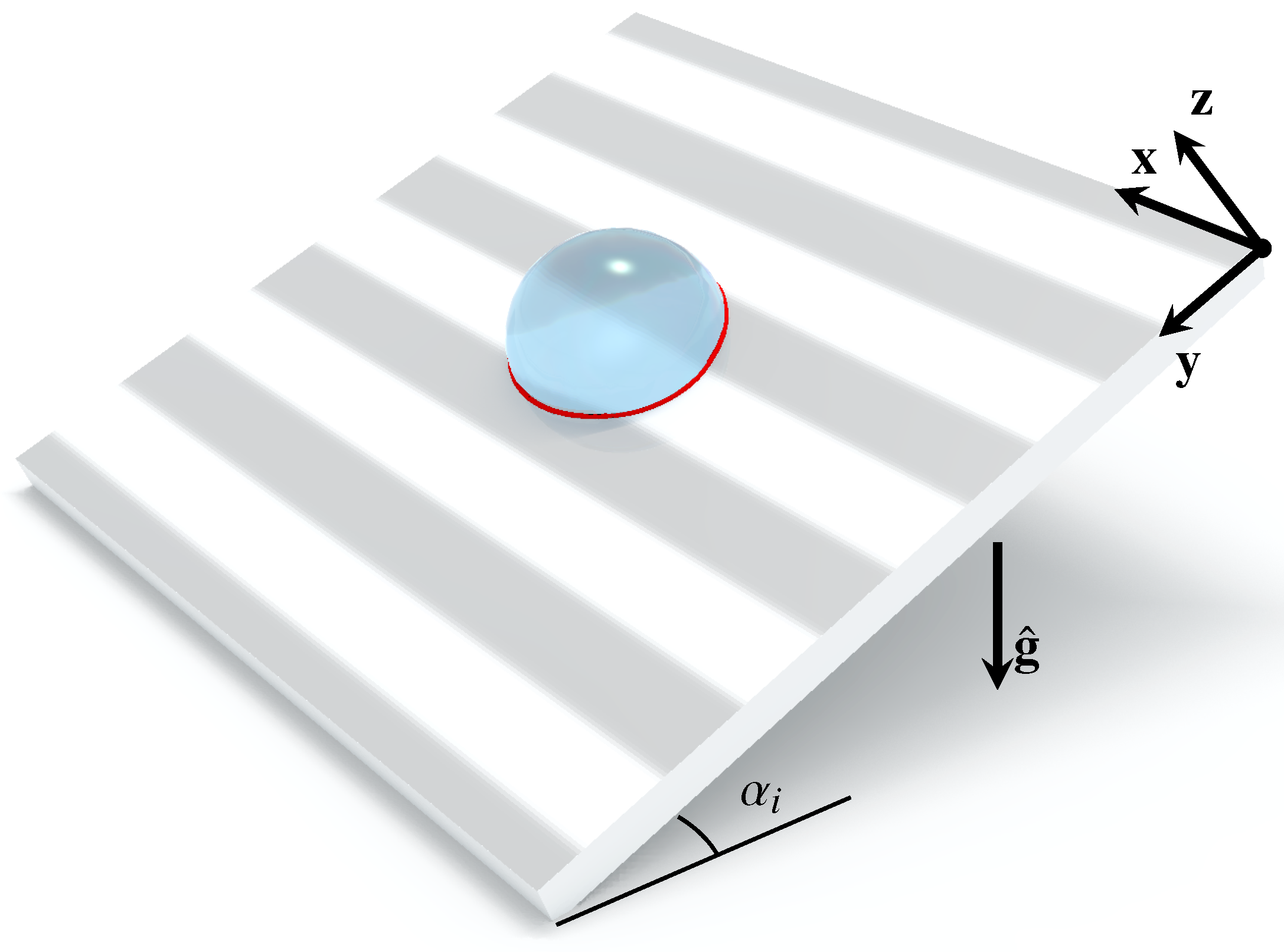
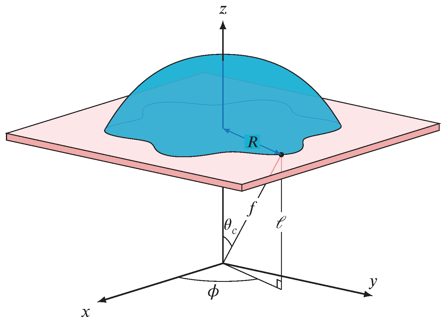
2.1. Governing Equations for DNS
2.2. Reduced-Order Model
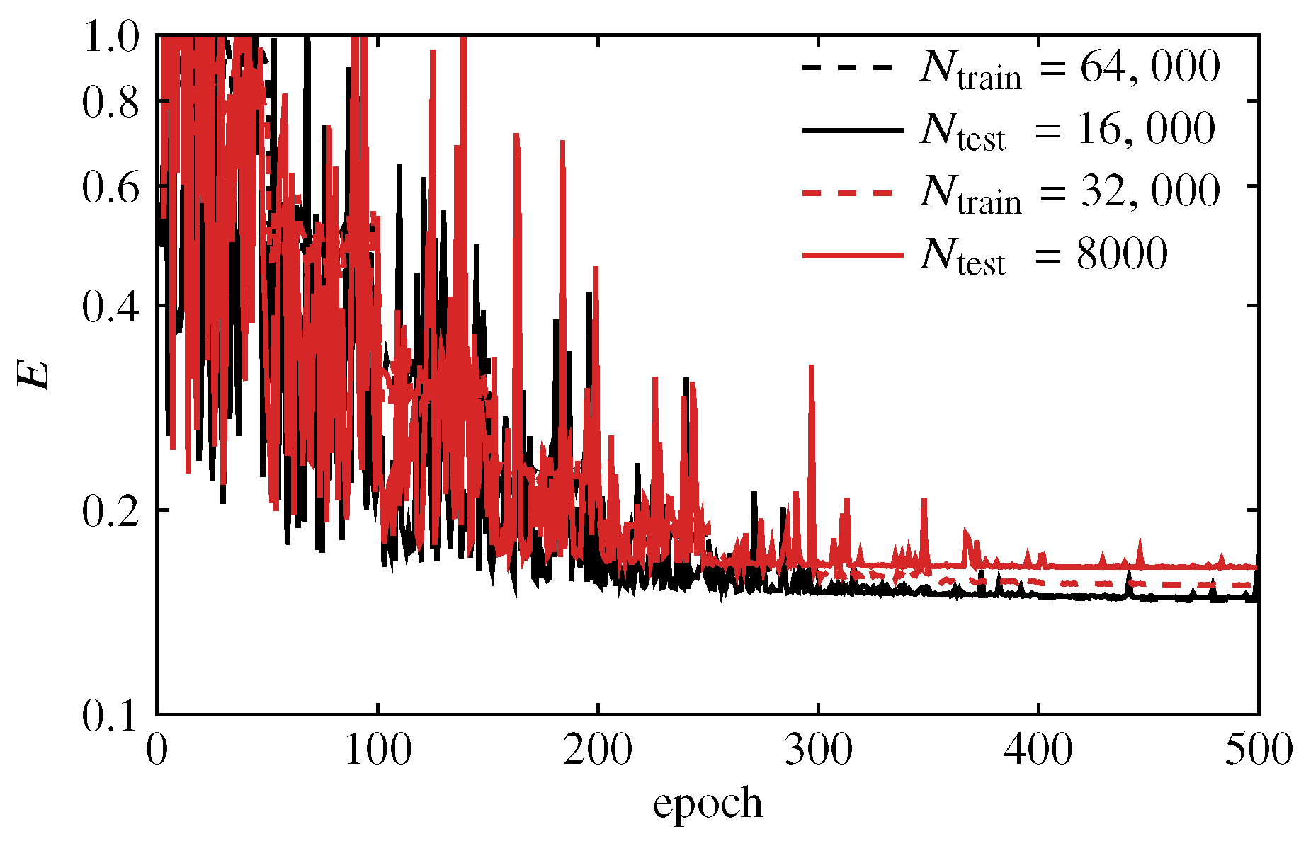
2.3. Data-Driven Method
2.4. Error Measure Based on the Fréchet Distance
3. Results
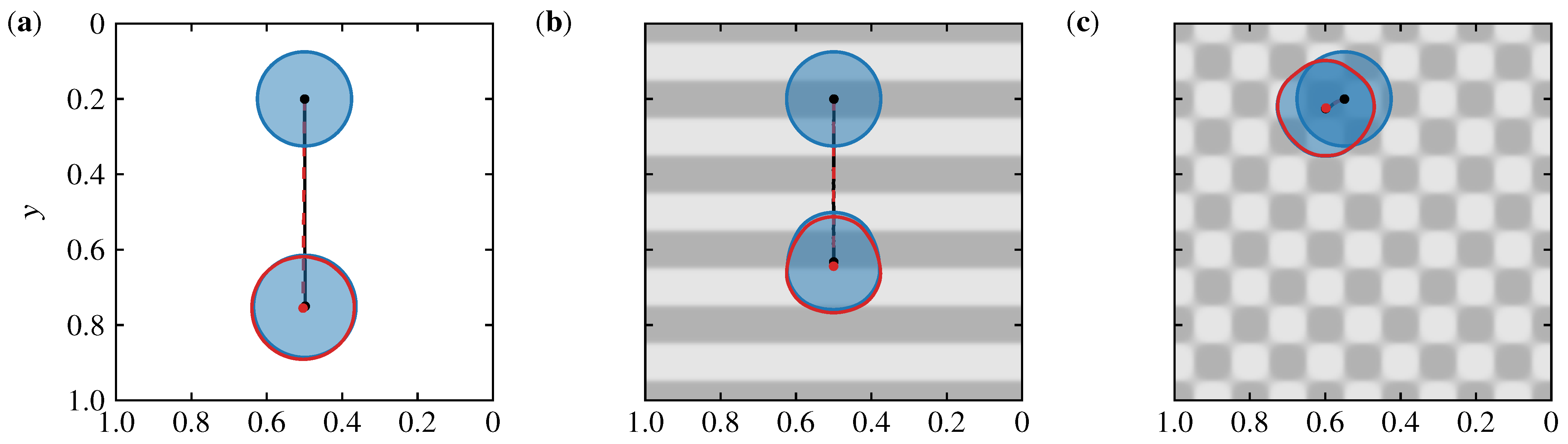
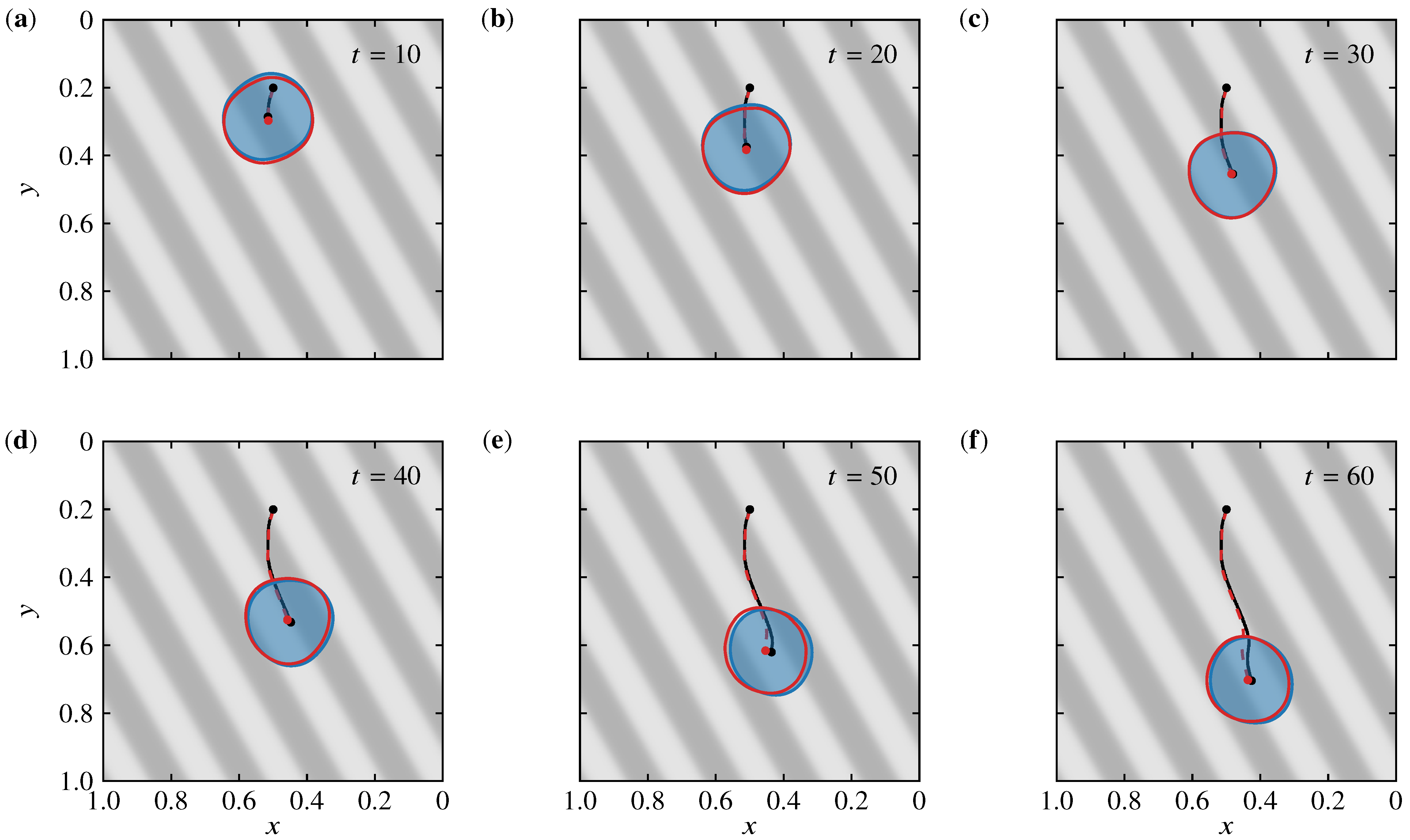
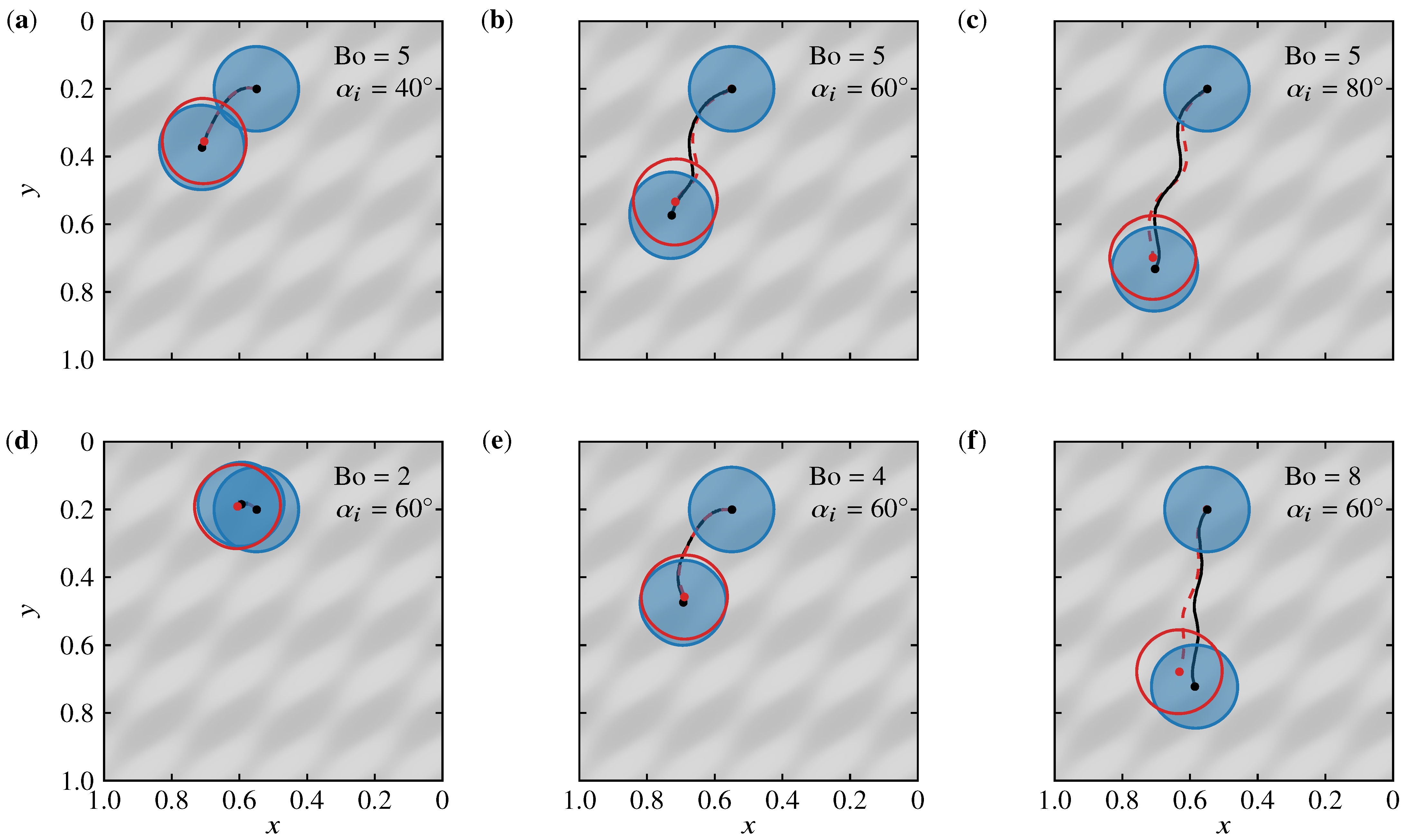
3.1. Modeling Parameters
- input data: , where the last term corresponds to the component of the acceleration of gravity on the -plane which is approximately normal to the contact line, and
- target data:
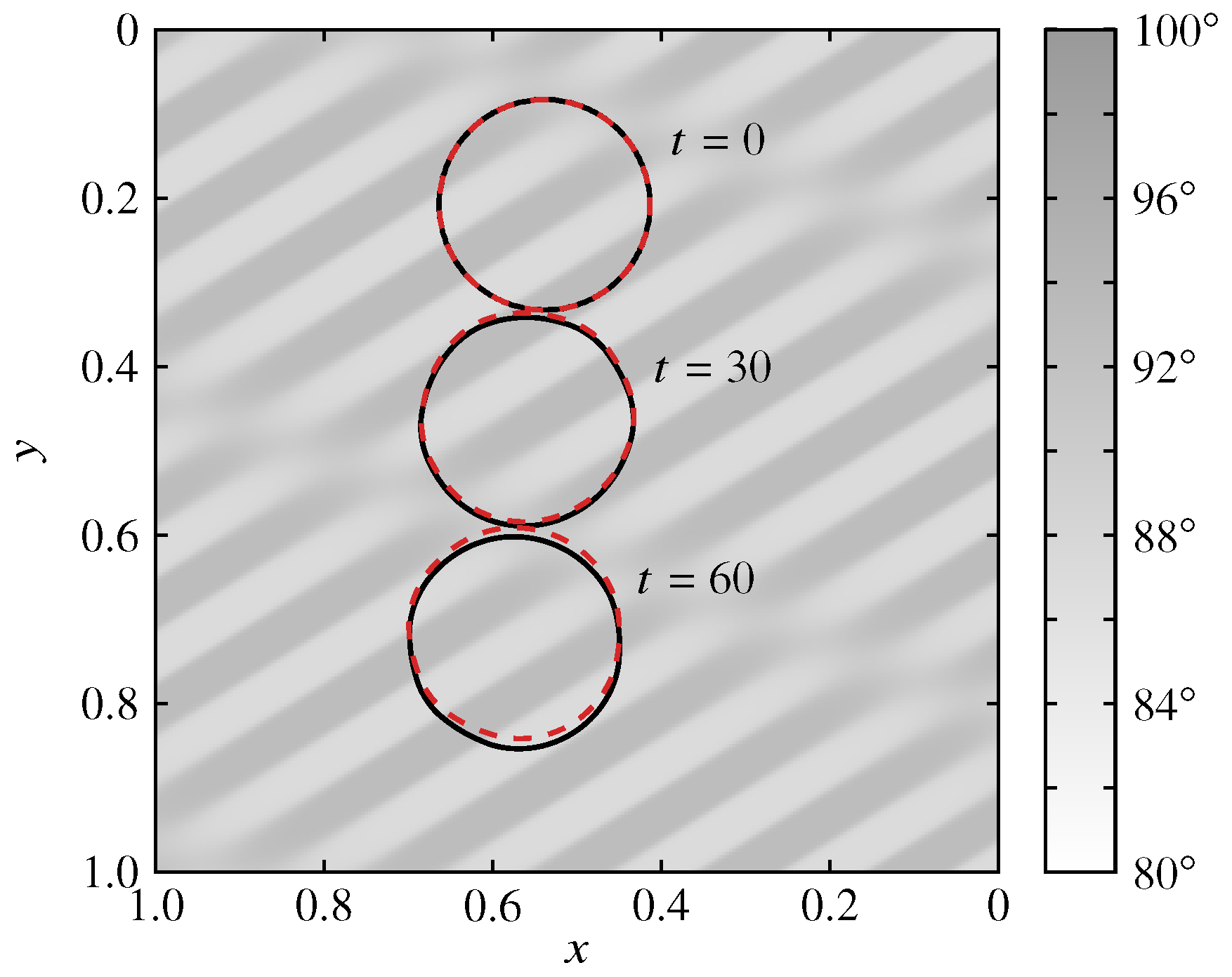
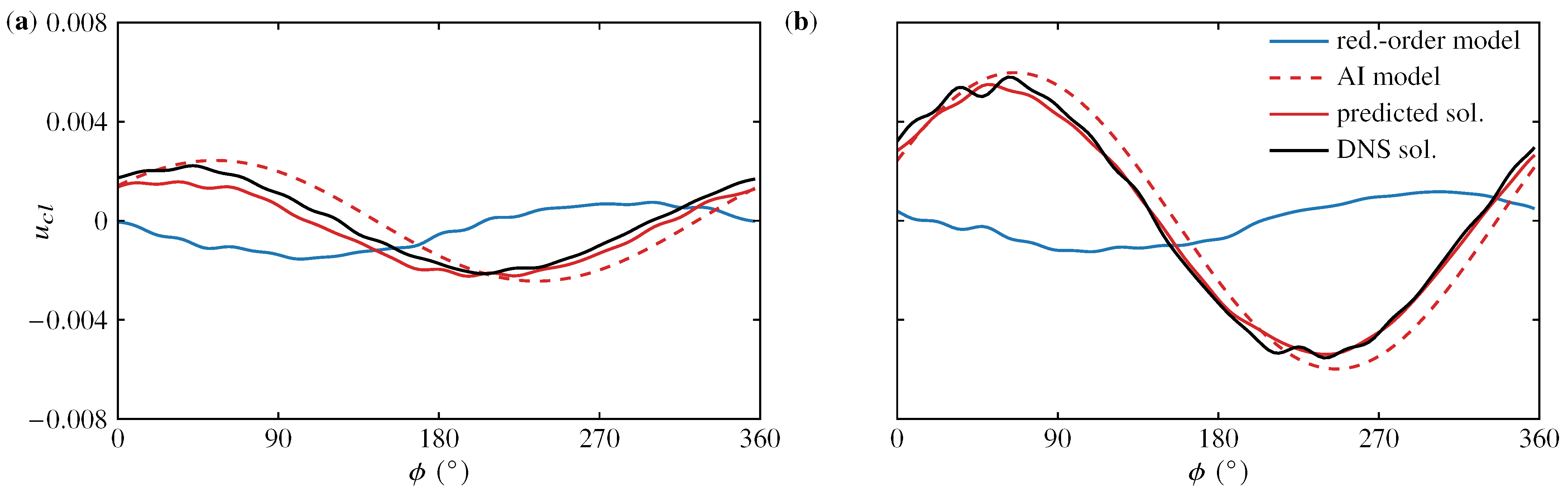
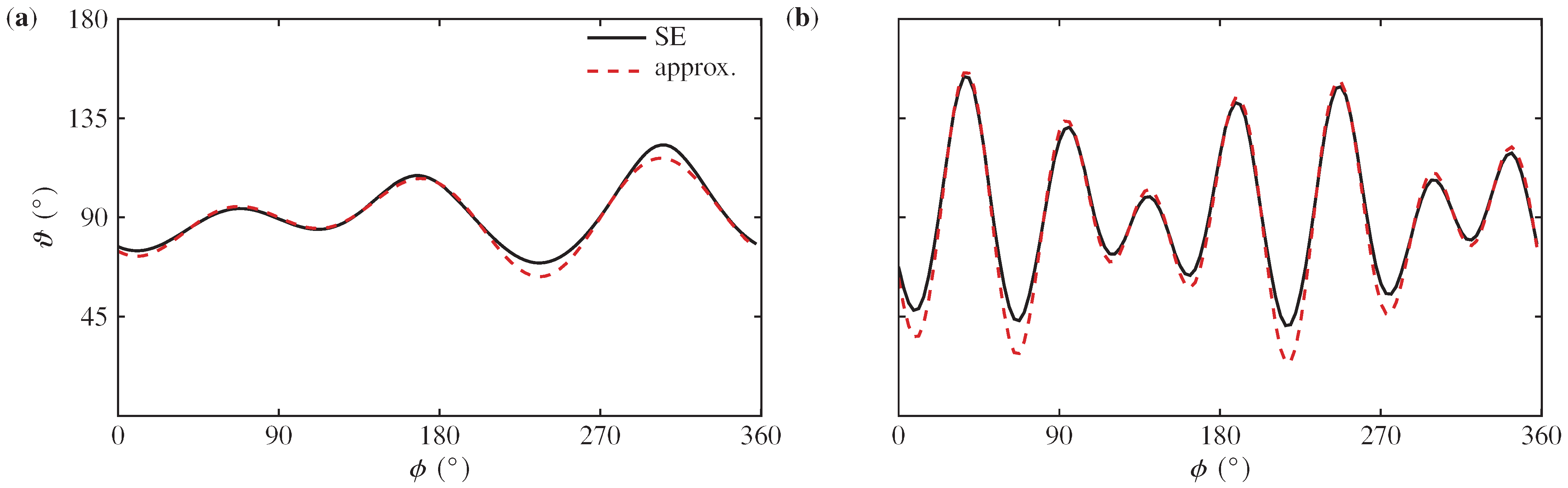
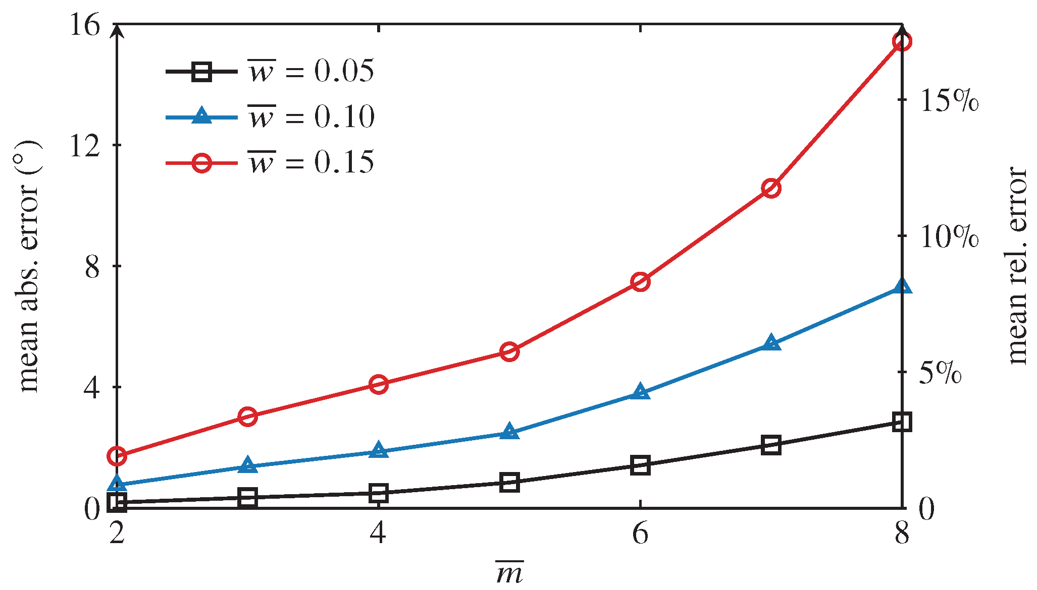
3.2. Tests
4. Conclusions
Author Contributions
Funding
Data Availability Statement
Acknowledgments
Conflicts of Interest
Abbreviations
| ReLU | rectified linear unit |
| PDE | partial differential equation |
| ODE | ordinary differential equation |
| CFD | computational fluid dynamics |
| DNS | direct numerical simulations |
| FNO | Fourier neural operator |
| CFL | Courant–Friedrichs–Lewy |
| AI | artificial intelligence |
Appendix A. Derivation of an Approximation to the Apparent Angle


References
- Moragues, T.; Arguijo, D.; Beneyton, T.; Modavi, C.; Simutis, K.; Abate, A.R.; Baret, J.C.; deMello, A.J.; Densmore, D.; Griffiths, A.D. Droplet-based microfluidics. Nat. Rev. Methods Prim. 2023, 3, 32. [Google Scholar] [CrossRef]
- Zhang, Y.; Dong, Z.; Li, C.; Du, H.; Fang, N.X.; Wu, L.; Song, Y. Continuous 3D printing from one single droplet. Nat. Commun. 2020, 11, 4685. [Google Scholar] [CrossRef]
- Bonn, D.; Eggers, J.; Indekeu, J.; Meunier, J.; Rolley, E. Wetting and spreading. Rev. Mod. Phys. 2009, 81, 739. [Google Scholar] [CrossRef]
- Wan, K.; Gou, X.; Guo, Z. Bio-inspired Fog Harvesting Materials: Basic Research and Bionic Potential Applications. J. Bionic Eng. 2021, 18, 501–533. [Google Scholar] [CrossRef]
- Podgorski, T.; Flesselles, J.M.; Limat, L. Corners, cusps, and pearls in running drops. Phys. Rev. Lett. 2001, 87, 036102. [Google Scholar] [CrossRef] [PubMed]
- Le Grand, N.; Daerr, A.; Limat, L. Shape and motion of drops sliding down an inclined plane. J. Fluid Mech. 2005, 541, 293–315. [Google Scholar] [CrossRef]
- Miwa, M.; Nakajima, A.; Fujishima, A.; Hashimoto, K.; Watanabe, T. Effects of the surface roughness on sliding angles of water droplets on superhydrophobic surfaces. Langmuir 2000, 16, 5754–5760. [Google Scholar] [CrossRef]
- ElSherbini, A.I.; Jacobi, A.M. Critical contact angles for liquid drops on inclined surfaces. In Surface and Colloid Science; Springer: Berlin/Heidelberg, Germany, 2004; pp. 57–62. [Google Scholar]
- Morita, M.; Koga, T.; Otsuka, H.; Takahara, A. Macroscopic-wetting anisotropy on the line-patterned surface of fluoroalkylsilane monolayers. Langmuir 2005, 21, 911–918. [Google Scholar] [CrossRef]
- Berejnov, V.; Thorne, R.E. Effect of transient pinning on stability of drops sitting on an inclined plane. Phys. Rev. E 2007, 75, 066308. [Google Scholar] [CrossRef] [PubMed]
- Suzuki, S.; Nakajima, A.; Tanaka, K.; Sakai, M.; Hashimoto, A.; Yoshida, N.; Kameshima, Y.; Okada, K. Sliding behavior of water droplets on line-patterned hydrophobic surfaces. Appl. Surf. Sci. 2008, 254, 1797–1805. [Google Scholar] [CrossRef]
- Bouteau, M.; Cantin, S.; Benhabib, F.; Perrot, F. Sliding behavior of liquid droplets on tilted Langmuir–Blodgett surfaces. J. Colloid Interface Sci. 2008, 317, 247–254. [Google Scholar] [CrossRef] [PubMed]
- Varagnolo, S.; Schiocchet, V.; Ferraro, D.; Pierno, M.; Mistura, G.; Sbragaglia, M.; Gupta, A.; Amati, G. Tuning drop motion by chemical patterning of surfaces. Langmuir 2014, 30, 2401–2409. [Google Scholar] [CrossRef] [PubMed]
- Chaudhury, M.K.; Whitesides, G.M. How to make water run uphill. Science 1992, 256, 1539–1541. [Google Scholar] [CrossRef] [PubMed]
- Brunet, P.; Eggers, J.; Deegan, R. Vibration-induced climbing of drops. Phys. Rev. Lett. 2007, 99, 144501. [Google Scholar] [CrossRef] [PubMed]
- Savva, N.; Kalliadasis, S. Droplet motion on inclined heterogeneous substrates. J. Fluid Mech. 2013, 725, 462–491. [Google Scholar] [CrossRef]
- Benilov, E.; Benilov, M. A thin drop sliding down an inclined plate. J. Fluid Mech. 2015, 773, 75–102. [Google Scholar] [CrossRef]
- Thiele, U.; Velarde, M.G.; Neuffer, K.; Bestehorn, M.; Pomeau, Y. Sliding drops in the diffuse interface model coupled to hydrodynamics. Phys. Rev. E 2001, 64, 061601. [Google Scholar] [CrossRef]
- Thiele, U.; Neuffer, K.; Bestehorn, M.; Pomeau, Y.; Velarde, M.G. Sliding drops on an inclined plane. Colloids Surfaces A Physicochem. Eng. Asp. 2002, 206, 87–104. [Google Scholar] [CrossRef]
- Thiele, U.; Knobloch, E. Driven drops on heterogeneous substrates: Onset of sliding motion. Phys. Rev. Lett. 2006, 97, 204501. [Google Scholar] [CrossRef]
- Koh, Y.; Lee, Y.; Gaskell, P.; Jimack, P.; Thompson, H. Droplet migration: Quantitative comparisons with experiment. Eur. Phys. J. Spec. Top. 2009, 166, 117–120. [Google Scholar] [CrossRef][Green Version]
- Afkhami, S.; Buongiorno, J.; Guion, A.; Popinet, S.; Saade, Y.; Scardovelli, R.; Zaleski, S. Transition in a numerical model of contact line dynamics and forced dewetting. J. Comput. Phys. 2018, 374, 1061–1093. [Google Scholar] [CrossRef]
- Cox, R. The dynamics of the spreading of liquids on a solid surface. Part 1. Viscous flow. J. Fluid Mech. 1986, 168, 169–194. [Google Scholar] [CrossRef]
- Dimitrakopoulos, P.; Higdon, J. On the gravitational displacement of three-dimensional fluid droplets from inclined solid surfaces. J. Fluid Mech. 1999, 395, 181–209. [Google Scholar] [CrossRef]
- Cavalli, A.; Musterd, M.; Mugele, F. Numerical investigation of dynamic effects for sliding drops on wetting defects. Phys. Rev. E 2015, 91, 023013. [Google Scholar] [CrossRef] [PubMed]
- Fullana, T.; Zaleski, S.; Popinet, S. Dynamic wetting failure in curtain coating by the Volume-of-Fluid method: Volume-of-Fluid simulations on quadtree meshes. Eur. Phys. J. Spec. Top. 2020, 229, 1923–1934. [Google Scholar] [CrossRef]
- Sakakeeny, J.; Ling, Y. Numerical study of natural oscillations of supported drops with free and pinned contact lines. Phys. Fluids 2021, 33, 062109. [Google Scholar] [CrossRef]
- Han, T.Y.; Zhang, J.; Tan, H.; Ni, M.J. A consistent and parallelized height function based scheme for applying contact angle to 3D volume-of-fluid simulations. J. Comput. Phys. 2021, 433, 110190. [Google Scholar] [CrossRef]
- Dupuis, A.; Yeomans, J. Dynamics of sliding drops on superhydrophobic surfaces. Europhys. Lett. 2006, 75, 105. [Google Scholar] [CrossRef]
- Varagnolo, S.; Ferraro, D.; Fantinel, P.; Pierno, M.; Mistura, G.; Amati, G.; Biferale, L.; Sbragaglia, M. Stick-slip sliding of water drops on chemically heterogeneous surfaces. Phys. Rev. Lett. 2013, 111, 066101. [Google Scholar] [CrossRef] [PubMed]
- Sbragaglia, M.; Biferale, L.; Amati, G.; Varagnolo, S.; Ferraro, D.; Mistura, G.; Pierno, M. Sliding drops across alternating hydrophobic and hydrophilic stripes. Phys. Rev. E 2014, 89, 012406. [Google Scholar] [CrossRef] [PubMed]
- Borcia, R.; Borcia, I.D.; Bestehorn, M. Drops on an arbitrarily wetting substrate: A phase field description. Phys. Rev. E 2008, 78, 066307. [Google Scholar] [CrossRef] [PubMed]
- Ramos, J.; Granato, E.; Ying, S.; Achim, C.; Elder, K.; Ala-Nissila, T. Dynamical transitions and sliding friction of the phase-field-crystal model with pinning. Phys. Rev. E 2010, 81, 011121. [Google Scholar] [CrossRef] [PubMed]
- Do Hong, S.; Ha, M.Y.; Balachandar, S. Static and dynamic contact angles of water droplet on a solid surface using molecular dynamics simulation. J. Colloid Interface Sci. 2009, 339, 187–195. [Google Scholar] [CrossRef] [PubMed]
- Berim, G.O.; Ruckenstein, E. Microscopic calculation of the sticking force for nanodrops on an inclined surface. J. Chem. Phys. 2008, 129, 114709. [Google Scholar] [CrossRef] [PubMed]
- Das, A.K.; Das, P.K. Simulation of drop movement over an inclined surface using smoothed particle hydrodynamics. Langmuir 2009, 25, 11459–11466. [Google Scholar] [CrossRef] [PubMed]
- Brunton, S.L.; Noack, B.R.; Koumoutsakos, P. Machine learning for fluid mechanics. Annu. Rev. Fluid Mech. 2020, 52, 477–508. [Google Scholar] [CrossRef]
- Sarghini, F.; De Felice, G.; Santini, S. Neural networks based subgrid scale modeling in large eddy simulations. Comput. Fluids 2003, 32, 97–108. [Google Scholar] [CrossRef]
- Ling, J.; Kurzawski, A.; Templeton, J. Reynolds averaged turbulence modelling using deep neural networks with embedded invariance. J. Fluid Mech. 2016, 807, 155–166. [Google Scholar] [CrossRef]
- Fukami, K.; Fukagata, K.; Taira, K. Super-resolution reconstruction of turbulent flows with machine learning. J. Fluid Mech. 2019, 870, 106–120. [Google Scholar] [CrossRef]
- Fukami, K.; Fukagata, K.; Taira, K. Super-resolution analysis via machine learning: A survey for fluid flows. Theor. Comput. Fluid Dyn. 2023, 37, 421–444. [Google Scholar] [CrossRef]
- Um, K.; Brand, R.; Fei, Y.R.; Holl, P.; Thuerey, N. Solver-in-the-loop: Learning from differentiable physics to interact with iterative pde-solvers. Adv. Neural Inf. Process. Syst. 2020, 33, 6111–6122. [Google Scholar]
- Wan, Z.Y.; Sapsis, T.P. Machine learning the kinematics of spherical particles in fluid flows. J. Fluid Mech. 2018, 857, R2. [Google Scholar] [CrossRef]
- Wan, Z.Y.; Karnakov, P.; Koumoutsakos, P.; Sapsis, T.P. Bubbles in turbulent flows: Data-driven, kinematic models with history terms. Int. J. Multiph. Flow 2020, 129, 103286. [Google Scholar] [CrossRef]
- Demou, A.D.; Savva, N. AI-assisted modeling of capillary-driven droplet dynamics. Data-Centric Eng. 2023, 4, e24. [Google Scholar] [CrossRef]
- Lacey, A. The motion with slip of a thin viscous droplet over a solid surface. Stud. Appl. Math. 1982, 67, 217–230. [Google Scholar] [CrossRef]
- Savva, N.; Groves, D.; Kalliadasis, S. Droplet dynamics on chemically heterogeneous substrates. J. Fluid Mech. 2019, 859, 321–361. [Google Scholar] [CrossRef]
- Tryggvason, G.; Scardovelli, R.; Zaleski, S. Direct Numerical Simulations of Gas–Liquid Multiphase Flows; Cambridge University Press: Cambridge, UK, 2011. [Google Scholar]
- Popinet, S. Gerris: A tree-based adaptive solver for the incompressible Euler equations in complex geometries. J. Comput. Phys. 2003, 190, 572–600. [Google Scholar] [CrossRef]
- Popinet, S. An accurate adaptive solver for surface-tension-driven interfacial flows. J. Comput. Phys. 2009, 228, 5838–5866. [Google Scholar] [CrossRef]
- Popinet, S. A quadtree-adaptive multigrid solver for the Serre–Green–Naghdi equations. J. Comput. Phys. 2015, 302, 336–358. [Google Scholar] [CrossRef]
- Afkhami, S.; Bussmann, M. Height functions for applying contact angles to 2D VOF simulations. Int. J. Numer. Methods Fluids 2008, 57, 453–472. [Google Scholar] [CrossRef]
- Afkhami, S.; Bussmann, M. Height functions for applying contact angles to 3D VOF simulations. Int. J. Numer. Methods Fluids 2009, 61, 827–847. [Google Scholar] [CrossRef]
- Popinet, S. Numerical models of surface tension. Annu. Rev. Fluid Mech. 2018, 50, 49–75. [Google Scholar] [CrossRef]
- Afkhami, S.; Zaleski, S.; Bussmann, M. A mesh-dependent model for applying dynamic contact angles to VOF simulations. J. Comput. Phys. 2009, 228, 5370–5389. [Google Scholar] [CrossRef]
- Sakakeeny, J.; Ling, Y. Natural oscillations of a sessile drop on flat surfaces with mobile contact lines. Phys. Rev. Fluids 2020, 5, 123604. [Google Scholar] [CrossRef]
- Negus, M.J.; Moore, M.R.; Oliver, J.M.; Cimpeanu, R. Droplet impact onto a spring-supported plate: Analysis and simulations. J. Eng. Math. 2021, 128, 3. [Google Scholar] [CrossRef]
- Marston, J.; Hawkins, V.; Decent, S.; Simmons, M. Influence of surfactant upon air entrainment hysteresis in curtain coating. Exp. Fluids 2009, 46, 549–558. [Google Scholar] [CrossRef]
- Liu, C.Y.; Carvalho, M.S.; Kumar, S. Dynamic wetting failure in curtain coating: Comparison of model predictions and experimental observations. Chem. Eng. Sci. 2019, 195, 74–82. [Google Scholar] [CrossRef]
- Kovachki, N.; Li, Z.; Liu, B.; Azizzadenesheli, K.; Bhattacharya, K.; Stuart, A.; Anandkumar, A. Neural operator: Learning maps between function spaces. arXiv 2021, arXiv:2108.08481. [Google Scholar]
- Li, Z.; Kovachki, N.; Azizzadenesheli, K.; Liu, B.; Bhattacharya, K.; Stuart, A.; Anandkumar, A. Fourier neural operator for parametric partial differential equations. arXiv 2020, arXiv:2010.08895. [Google Scholar]
- Alt, H.; Godau, M. Computing the Fréchet distance between two polygonal curves. Int. J. Comput. Geom. Appl. 1995, 5, 75–91. [Google Scholar] [CrossRef]
- Brakke, K.A. The surface evolver. Exp. Math. 1992, 1, 141–165. [Google Scholar] [CrossRef]
- Humplik, T.; Lee, J.; O’hern, S.; Fellman, B.; Baig, M.; Hassan, S.; Atieh, M.; Rahman, F.; Laoui, T.; Karnik, R.; et al. Nanostructured materials for water desalination. Nanotechnology 2011, 22, 292001. [Google Scholar] [CrossRef] [PubMed]
- Lee, A.; Moon, M.W.; Lim, H.; Kim, W.D.; Kim, H.Y. Water harvest via dewing. Langmuir 2012, 28, 10183–10191. [Google Scholar] [CrossRef] [PubMed]
- Sobac, B.; Brutin, D. Desiccation of a sessile drop of blood: Cracks, folds formation and delamination. Colloids Surf. A Physicochem. Eng. Asp. 2014, 448, 34–44. [Google Scholar] [CrossRef]
- Hartmann, S.; Diddens, C.; Jalaal, M.; Thiele, U. Sessile drop evaporation in a gap – crossover between diffusion-limited and phase transition-limited regime. J. Fluid Mech. 2023, 960, A32. [Google Scholar] [CrossRef]


| w | ||||
|---|---|---|---|---|
| 32 | 0.203 | 0.183 | 0.164 | 0.153 |
| 64 | 0.203 | 0.182 | 0.165 | 0.149 |
| 128 | 0.204 | 0.174 | 0.164 | 0.151 |
| 256 | 0.205 | 0.169 | 0.163 | 0.152 |
Disclaimer/Publisher’s Note: The statements, opinions and data contained in all publications are solely those of the individual author(s) and contributor(s) and not of MDPI and/or the editor(s). MDPI and/or the editor(s) disclaim responsibility for any injury to people or property resulting from any ideas, methods, instructions or products referred to in the content. |
© 2024 by the authors. Licensee MDPI, Basel, Switzerland. This article is an open access article distributed under the terms and conditions of the Creative Commons Attribution (CC BY) license (https://creativecommons.org/licenses/by/4.0/).
Share and Cite
Demou, A.D.; Savva, N. Hybrid AI-Analytical Modeling of Droplet Dynamics on Inclined Heterogeneous Surfaces. Mathematics 2024, 12, 1188. https://doi.org/10.3390/math12081188
Demou AD, Savva N. Hybrid AI-Analytical Modeling of Droplet Dynamics on Inclined Heterogeneous Surfaces. Mathematics. 2024; 12(8):1188. https://doi.org/10.3390/math12081188
Chicago/Turabian StyleDemou, Andreas D., and Nikos Savva. 2024. "Hybrid AI-Analytical Modeling of Droplet Dynamics on Inclined Heterogeneous Surfaces" Mathematics 12, no. 8: 1188. https://doi.org/10.3390/math12081188
APA StyleDemou, A. D., & Savva, N. (2024). Hybrid AI-Analytical Modeling of Droplet Dynamics on Inclined Heterogeneous Surfaces. Mathematics, 12(8), 1188. https://doi.org/10.3390/math12081188