Gradient Weakly Sensitive Multi-Source Sensor Image Registration Method

Abstract

Aiming at the nonlinear radiometric differences between multi-source sensor images and coherent spot noise and other factors that lead to alignment difficulties, the registration method of gradient weakly sensitive multi-source sensor images is proposed, which does not need to extract the image gradient in the whole process and has rotational invariance. In the feature point detection stage, the maximum moment map is obtained by using the phase consistency transform to replace the gradient edge map for chunked Harris feature point detection, thus increasing the number of repeated feature points in the heterogeneous image. To have rotational invariance of the subsequent descriptors, a method to determine the main phase angle is proposed. The phase angle of the region near the feature point is counted, and the parabolic interpolation method is used to estimate the more accurate main phase angle under the determined interval. In the feature description stage, the Log-Gabor convolution sequence is used to construct the index map with the maximum phase amplitude, the heterogeneous image is converted to an isomorphic image, and the isomorphic image of the region around the feature point is rotated by using the main phase angle, which is in turn used to construct the feature vector with the feature point as the center by the quadratic interpolation method. In the feature matching stage, feature matching is performed by using the sum of squares of Euclidean distances as a similarity metric. Finally, after qualitative and quantitative experiments of six groups of five pairs of different multi-source sensor image alignment correct matching rates, root mean square errors, and the number of correctly matched points statistics, this algorithm is verified to have the advantage of robust accuracy compared with the current algorithms.

1. Introduction

The fusion of multi-source image data can obtain richer remote sensing information and has been widely used in the field of remote sensing [1,2,3]. The basic task of fusing two types of images to obtain richer information is to align them, but heterogeneous remote sensing images exist in the scale, rotation, radiation, noise, resolution, spatial-temporal, and phase differences, which makes it more difficult to be aligned [4,5]. Although satellite remote sensing data provide spatial calibration information (spatial reference) such as latitude, longitude, map grid, etc., the spatial references of different satellites or sensors are not consistent, which can cause several pixel differences. These small differences can lead to inaccurate feature correspondences in multi-source images, which can cause a decrease in the accuracy of image processing results in applications such as data fusion, collaborative classification, change detection, and image stitching. Therefore, it is particularly important to investigate effective, general, and robust image alignment algorithms. Three challenges need to be addressed [6]: (1) different geometric properties. For example, the side-view and measurement distance modes of Synthetic Aperture Radar (SAR) sensors will lead to a series of geometric aberrations [7,8]; (2) different radiation characteristics [9]. For example, SAR instruments are active remote sensing systems, while optical instruments are passive systems. The brightness values change significantly due to changes in imaging conditions; (3) spot noise generated by sensors [10], such as sensor and environmental noise, which make feature extraction in SAR images sleepy.

Mainstream image alignment algorithms are currently classified into two types [11]: region-based alignment methods and feature-based alignment methods. Region-based methods use image grayscale to directly compare template regions concerning each other or mutual information. Ye Yuanxin et al. [12] proposed a Histogram of Orientated Phase Congruency (HOPC) feature descriptor and utilized a region template-based alignment method to match feature points to achieve high accuracy in aligning optical and SAR images, and their algorithm is not rotationally invariant but relies on geographic location information. Xiang et al. [13] used two operators to compute the gradient of heterogeneous images and constructed a GLOH (gradient location and orientation histogram) descriptor for feature matching. Their algorithm is rotationally invariant and has a better alignment effect for high-resolution optical and SAR images, but the algorithm is not universally applicable. Its algorithm is rotationally invariant and has a good registration effect for high-resolution optical images and SAR images, but its generalization is poor and its algorithm copes with the environment limited to optical images and SAR images. The feature-based approach extracts point, contour line, and region features and matches them based on some similarity metric. For example, Chen et al. [14] proposed a Partial Intensity Invariant Feature Descriptor (the Partial Intensity Invariant Feature Descriptor, PIIFD) for multi-source retinal image alignment, which has intensity and rotation invariance, but the alignment accuracy is not high. Li [15] proposed a Radiation Insensitive Feature Transformation (RIFT) for Maximum Index Mapping (MIM) of feature description with high-intensity invariance but poor rotational invariance.

The current multi-source sensor image registration algorithms deal with the problem of homogenization and face poor multi-scene universality. Moreover, most of the descriptors with rotational invariance are built based on the image gradient, which can lead to the gradient inversion phenomenon, resulting in registration failure. Therefore, a weakly gradient-sensitive alignment method for multi-source sensor images is proposed to adapt to a variety of complex alignment environments. There is no need to extract the image gradient in the whole process and it has rotational invariance, which ensures the robustness of the present algorithm to nonlinear radiance differences and the registration accuracy under multi-source sensors.

2. Feature Point Extraction

The number of repeatable feature points between multi-source sensor images is critical to the success of the registration. The Harris operator can extract image corners as feature points, but the results of using the Harris operator to directly extract corner features for multi-source images do not have high stability and repeatability. 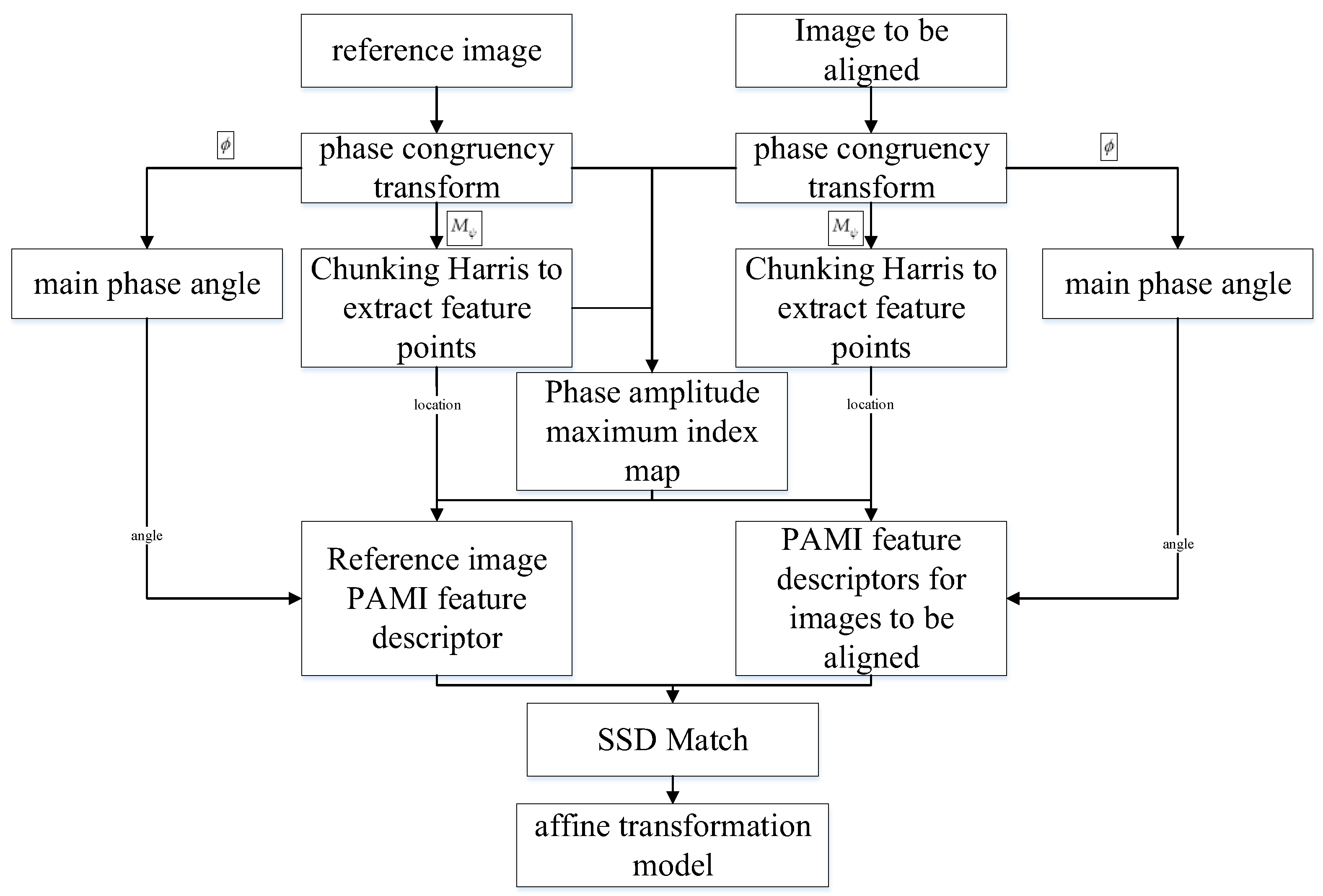Because phase information is highly invariant to image contrast, brightness, scale, and other variations [16], the use of phase information in the feature point extraction stage can detect more duplicate feature points (i.e., points with the same name) in multi-source images [17], which provides an a priori condition for the subsequent increase in the matching rate. In this paper, the maximum moment map obtained after phase congruence transformation is used to replace the intensity edge map, and the chunked Harris method is used for feature detection to enhance its robustness. The specific alignment process is shown in Figure 1:

In Figure 1, the specific flow of the realization of this algorithm is presented. As this paper adopts the feature alignment method, the dimensions of the reference image and the image to be aligned need to be larger than 96 × 96.

2.1. Phase Congruence Transformation

Phase congruence [18] is a frequency domain treatment based on phase considerations. The phase congruence is directly proportional to the local energy, and a commonly used step location method is based on the local energy extremes. A 2D Log-Gabor filter is used for phase congruence transformation.

The wavelet directional response is formed using the directional properties inherent in the 2D Log-Gabor filters [19,20] to generate the response map. The 2D Log-Gabor function is defined as follows:

$$L(\rho ,\theta ,s,\mathrm{o})=e^{\frac{-{(\rho -{\rho }_s)}^2}{2{\sigma }_{\rho }^2}}\times e^{\frac{-{(\theta -{\theta }_{so})}^2}{2{\sigma }_{\theta }^2}}$$

(1)

$${\rho }_s={\log }_2(n)-s$$

(2)

$${\theta }_{so}=\left\{\begin{array}{l}\frac{\pi }{n_o}\times o\begin{array}{cc}\begin{array}{cc} & \begin{array}{cc} & \end{array}\end{array}& s\in 2k+1\end{array}\\ \frac{\pi }{n_o}\times (o+\frac{1}{2})\begin{array}{cc}\begin{array}{cc}\begin{array}{cc} & \end{array}& \end{array}& \mathrm{s}\in 2\mathrm{k}\end{array}\end{array}\right.$$

(3)

$$({\sigma }_{\rho },{\sigma }_{\theta })=0.996(\sqrt{\frac{2}{3}},\sqrt{\frac{1}{2}}\times \frac{\pi }{n_o})$$

(4)

where $(\rho ,\theta )$ denotes the logarithmic polar coordinates, $n_o$ is the number of defined directions ranging from 3 to 20, which takes the value of 6 in this paper, $n$ denotes the size, and Equation (2) denotes the composition of the filter under n size, $s$ and $o$ are the scale and the direction of Log-Gabor, k is an integer number, $({\rho }_s,{\theta }_{so})$ is the center coordinates of the Log-Gabor filter, and ${\sigma }_{\rho }$ and ${\sigma }_{\theta }$ are the bandwidths under $\rho$ and $\theta$, respectively.

The 2D Log-Gabor belongs to the frequency domain filters and its corresponding spatial domain can be obtained by the inverse Fourier transform. In the spatial domain, the 2D Log-Gabor can be expressed as:

$$L(x,y,s,o)=L_{even}(x,y,s,o)+i{L}_{odd}(x,y,s,o)$$

(5)

In Equation (5), $L_{even}(x,y,s,o)$ and $L_{odd}(x,y,s,o)$ represent even-symmetric and odd-symmetric filters of size 3 × 3, respectively, and both have good local and directional characteristics.

Setting $I(x,y)$ represents a two-dimensional image signal. The image $I(x,y)$ is convolved with even-symmetric and odd-symmetric filters to obtain the response components $E_{so}(x,y)$ and $O_{so}(x,y)$:

$$\left[E_{so}(x,y),O_{so}(x,y)\right]=\left[\begin{array}{l}I(x,y)\times L^{even}(x,y,s,o),\\ I(x,y)\times L^{odd}(x,y,s,o)\end{array}\right]$$

(6)

$I(x,y)$ amplitude component $A_{so}(x,y)$ and phase component $\varphi$ at scale $s$ and orientation $o$:

$$A_{so}(x,y)=\sqrt{E_{so}{(x,y)}^2+O_{so}{(x,y)}^2}$$

(7)

$${\varphi }_{so}(x,y)=\arctan (\frac{O_{so}(x,y)}{E_{so}(x,y)})$$

(8)

Considering the results of the analyses in all directions and introducing the noise compensation term T, the final 2D phase congruency transformation model is:

$$PC(x,y)=\frac{{\displaystyle \sum _s{\displaystyle \sum _o{\omega }_o(x,y)\times }}⌊A_{so}(x,y)\times \mathrm{\Delta }{\varphi }_{so}(x,y)-T⌋}{{\displaystyle \sum _s{\displaystyle \sum _o{A}_{so}(x,y)+\xi }}}$$

(9)

In Equation (9), ${\omega }_o(x,y)$ is a weighting function; $\xi$ is a small value taken as 0.001; and operation ⌊ ⌋ prevents the closure quantity from obtaining a negative value and takes zero when the closure quantity is negative. $\mathrm{\Delta }{\varphi }_{so}(x,y)$ is the phase deviation function with $A_{so}(x,y)$, and the product can be expressed as:

$$A_{so}(x,y)\times \mathrm{\Delta }{\varphi }_{so}(x,y)=(E_{so}(x,y){\overline{\varphi }}_E(x,y)+O_{so}(x,y){\overline{\varphi }}_O(x,y))-\left|E_{so}(x,y){\overline{\varphi }}_O(x,y)-O_{so}(x,y){\overline{\varphi }}_E(x,y)\right|$$

(10)

In Equation (10),

$${\overline{\varphi }}_E(x,y)={\displaystyle \sum _s{\displaystyle \sum _o\frac{E_{so}(x,y)}{C(x,y)}}}$$

(11)

$${\overline{\varphi }}_O(x,y)={\displaystyle \sum _s{\displaystyle \sum _o\frac{O_{so}(x,y)}{C(x,y)}}}$$

(12)

$$C(x,y)=\sqrt{{({\displaystyle \sum _s{\displaystyle \sum _o{E}_{so}(x,y)}})}^2+{({\displaystyle \sum _s{\displaystyle \sum _o{O}_{so}(x,y)}})}^2}$$

(13)

2.2. Maximum Moment Map Feature Point Extraction

Based on Equation (9), very accurate response values can be obtained, i.e., the phase consistency value $PC(x,y)$. However, the effect of orientation changes on phase coherence measurements is neglected. To obtain a relationship between phase coherence measurements and orientation changes, an independent phase coherence response value equal to $PC({\theta }_o)$ is calculated for each orientation $o$, where ${\theta }_o$ is the angle of the orientation $o$. Calculate the maximum moments of these phase coherence plots and analyses the variation of moments with orientation.

According to the moment analysis algorithm, the magnitude of the maximum moment usually reflects the uniqueness of the line features. Three intermediate quantities are computed before the maximum moment $M_{\mathrm{\Psi }}$ is computed:

$$a={{\displaystyle \sum _o(PC({\theta }_o)\cos ({\theta }_o))}}^2$$

(14)

$$b=2{\displaystyle \sum _o(PC({\theta }_o)\cos ({\theta }_o))}(PC({\theta }_o)\sin ({\theta }_o))$$

(15)

$$c={\displaystyle \sum _{o}PC({\theta }_o)\sin {({\theta }_o)}^2}$$

(16)

The maximum moment $M_{\mathrm{\Psi }}$ is given by the following equation:

$$M_{\mathrm{\Psi }}=\frac{1}{2}(c+a+\sqrt{b^2+{(a-c)}^2})$$

(17)

$$\mathrm{\Psi }=\frac{1}{2}\arctan (\frac{b}{a-c})$$

(18)

In Equation (18), $\mathrm{\Psi }$ is the angle of the principal axis and $M_{\mathrm{\Psi }}$ is the value of the maximum moment concerning the direction, which corresponds to reflecting the edge characteristics of the image.

Due to the better radiation distortion resistance of the edge structure information, the maximum moment $M_{\mathrm{\Psi }}$ is used to detect the edge feature points. Chunked Harris feature detection using pair $M_{\mathrm{\Psi }}$ is equivalent to dividing the image to be detected into N × N non-overlapping square image blocks, calculating the Harris feature value of each pixel within the image block, and taking the first m points with the largest feature values within the image block as feature points.

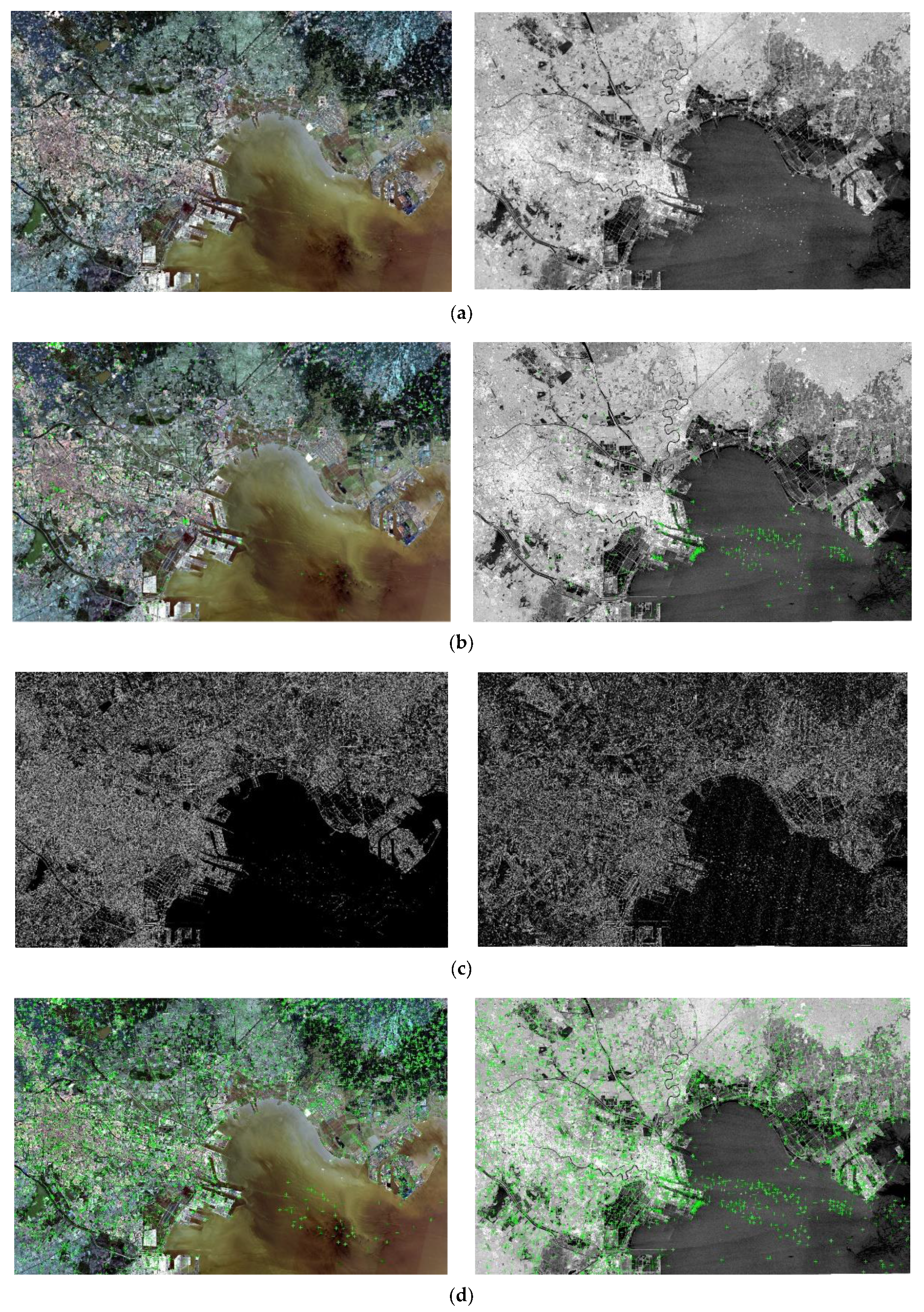
Figure 2 shows the results of feature detection; the green points in the figure are the detected feature points, and the more feature points, the greater the number of correct matching points for subsequent alignment. Figure 2a is a pair of heterogeneous remote sensing images and the comparison can be seen that the two images are very different, especially the SAR image by the noise interference, which is heavier. Figure 2b is the original map directly with the Harris feature detection results, and the results appear to fall into the phenomenon of local extremes. Since the map repeats the feature points less, it is difficult to ensure the accuracy of the alignment. Figure 2c is the maximum moment mapping map, and Figure 2d,e is the maximum moment mapping using the Harris and the chunked Harris operator feature detection results, respectively. Comparing Figure 2b,d, it is found that the Harris detector, a conventional feature detector based on image intensity, is very sensitive to nonlinear radial distortion, and the results do not have a large number of repeating feature points, whereas the maximum moment map obtained by the phase coherence transform has a good resistance to nonlinear radial distortion. By using the same Harris detector for the maximum moment map, a large number of reliable feature points can be obtained. As can be seen from Figure 2d,e, the feature points detected using the chunked Harris operator are more uniform. Therefore, replacing the maximum moment feature with the intensity edge map and using the chunked Harris operator for feature detection ensures the high repeatability of the features and provides a priori conditions for subsequent feature matching.

3. Feature Point Description

3.1. Determination of the Main Phase Angle

In existing methods, their algorithms are guaranteed to have rotational invariance by calculating a local second-order gradient to assign a principal direction $[0,2\pi ]$ to each feature point. However, due to the large nonlinear radiometric variation of the image, the principal direction extracted with the gradient is inherently inaccurate, and in multi-source sensor images, the gradient of the corresponding part of the image will sometimes change the direction by exactly 180°, which is very common and is called gradient inversion. To bypass the gradient information when extracting the principal direction and to suppress the gradient inversion phenomenon, the principal phase angle $[0,2\pi ]$ is used instead of the principal direction, thus making the descriptor rotationally invariant. 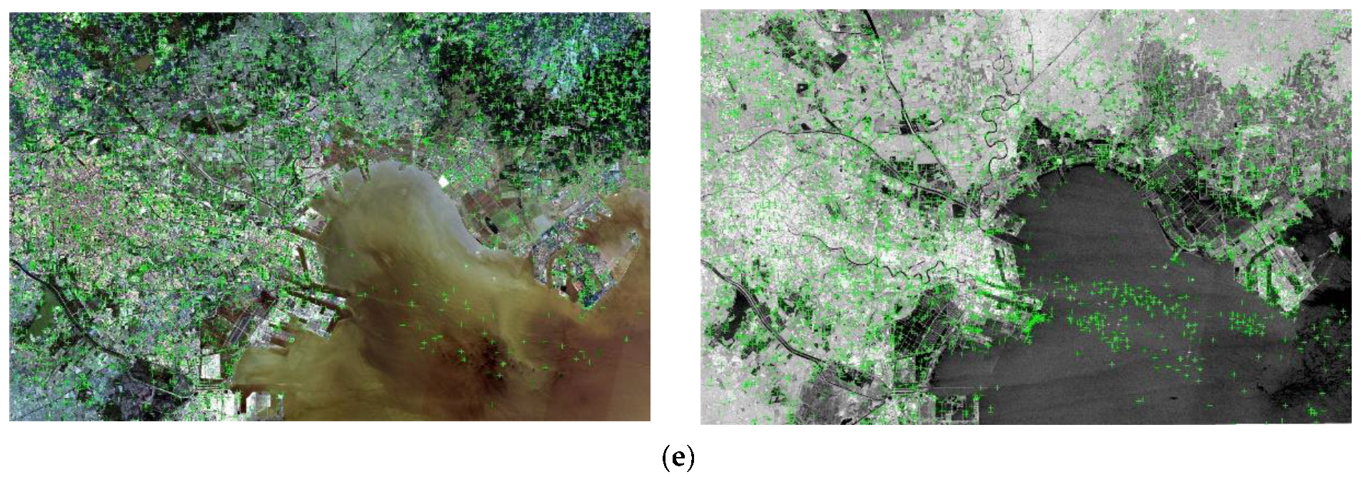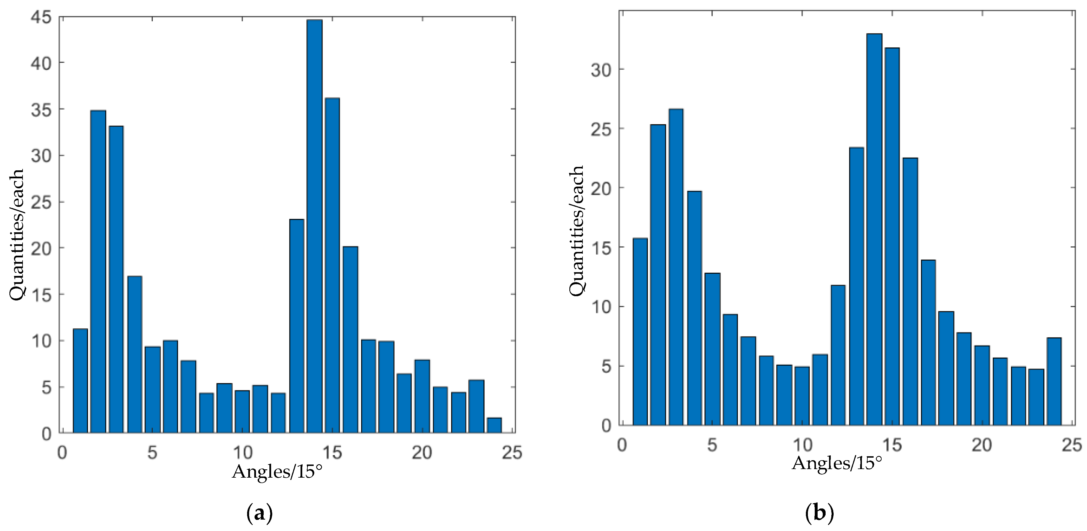The phase angle $\varphi$ of each pixel point in the image is obtained from Equation (8), and since the closer the feature point is to the neighborhood of the feature point the greater the impact on the feature matching, the phase angle of the circular region with a radius of 48 near each feature point is Gaussian-weighted and counted with a histogram of the phase angle, which divides the 360° into 24 columns, each of which is 15°. The histogram statistics of the phase angle in the region near a feature point in the image are shown in Figure 3, where the horizontal coordinate is the angle and the vertical coordinate is the number of statistics.

The histogram statistics of the phase angle in the region near a feature point in the image are shown in Figure 3, Figure 3a, to determine the interval in which the main phase angle is located, since at this point, $bin$ is a discrete parabolic interpolation which is needed based on the value near the maximum $bin$. (b) obtained after Gaussian smoothing in (a), which is intended to facilitate subsequent interpolation to estimate a more accurate main phase angle and to prevent sudden changes, thus using parabolic interpolation to estimate the main phase angle. The histogram of the smoothed phase angle is shown in Figure 3, and it can be concluded that the smoothing will not change the results of the interval where $bi{n}_{\max }$ is located, and it will be easier and more accurate to fit the local parabola.

Setting $bi{n}_{\max }$ as the vertex of the parabola gives the following:

$$bi{n}_{\max }=\frac{1}{2}\frac{\left(bi{n}_2^2-bi{n}_3^2\right)g_1+\left(bi{n}_3^2-bi{n}_1^2\right)g_2+\left(bi{n}_2^2-bi{n}_3^2\right)g_3}{(bi{n}_2-bi{n}_3)g_1+(bi{n}_3-bi{n}_1)g_2+(bi{n}_1-bi{n}_2)g_3}$$

(19)

$bi{n}_{2,1,3}$ denote the statistically maximal direction as well as the two directions around the maximal direction, and $g_{2,1,3}$ are the number of corresponding vertical coordinates of $b_{2,1,3}$. For example, in Figure 3b, $bi{n}_1=13$, $bi{n}_2=14$, and $bi{n}_3=15$, and the $bi{n}_{\max }$ estimate can be found by substituting into Equation (19).

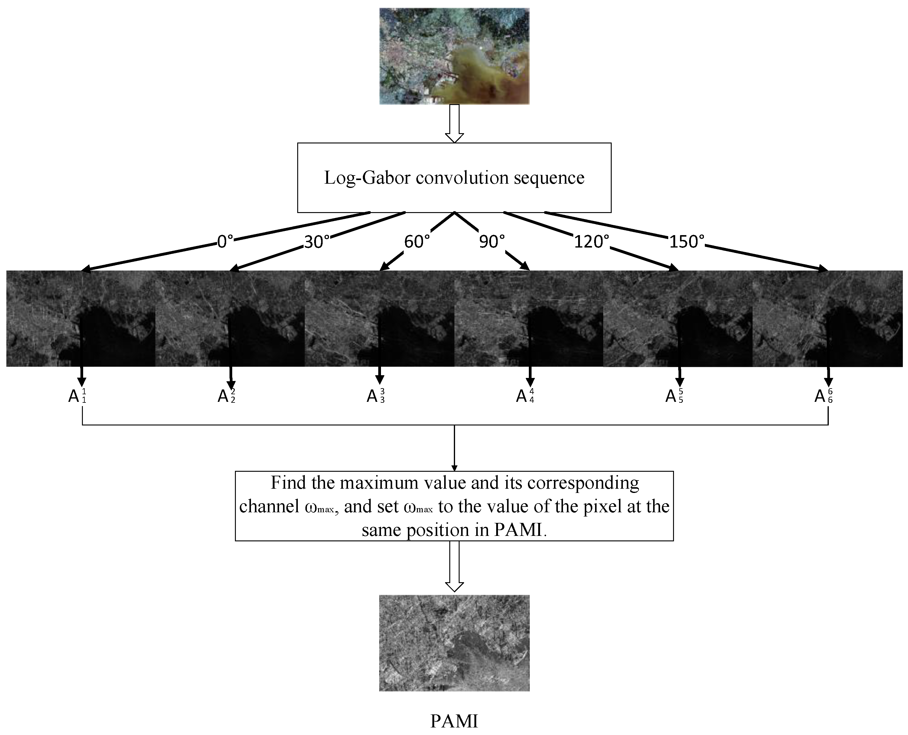
3.2. Creating the Phase-Amplitude Maximum Index Map

The phase-amplitude maximum index (PAMI) map is constructed from Log-Gabor convolutional sequences. The convolution sequence is obtained at the phase coherence detection stage. The first layer of the Log-Gabor convolution sequence is the convolution result in the $0^{°}$ direction (the initial layer of the convolution sequence), the second layer is ${30}^{°}$, and until the sixth layer is the convolution result in the ${150}^{°}$ direction. Figure 4 shows the construction flow of PAMI.

The convolution sequence utilized in Figure 4 is constructed as follows: first, given an image $I(x,y)$, $I(x,y)$ is convolved with a two-dimensional Log-Gabor filter (filter size 3 × 3) to obtain the response components $E_{so}(x,y)$ and $O_{so}(x,y)$; second, the amplitude $A_{so}(x,y)$ at scale $s$ and orientation $o$ is then computed, and different scales of the same orientation are summed to obtain the Log-Gabor convolution layer $A_o(x,y)$:

$$A_o(x,y)={\displaystyle \sum _{n=1}^{N_s}{A}_{so}(x,y)}$$

(20)

Finally, the Log-Gabor convolution sequence is obtained by arranging the Log-Gabor convolution layers in the order of direction, which belongs to the multi-channel convolution mapping ${\{A_o^{\omega }(x,y)\}}_1^{N_o}$, where $N_0$ is the number of directions and $\omega =1,2,\dots ,N_o$ denotes the different channels of the Log-Gabor convolution sequence. From the convolution results, for pixel $(x_{\mathrm{i}},y_j)$, a dimensional array ${\{A_o^{\omega }(x_{\mathrm{i}},y_j)\}}_1^{N_o}$ can be obtained, after which the maximum value $A_{\max }$ in the array is found corresponding to the position channel ${\omega }_{\max }$, and ${\omega }_{\max }$ is set to the pixel value of position $(x_{\mathrm{i}},y_j)$ in PAMI.

3.3. Creating the PAMI Descriptor

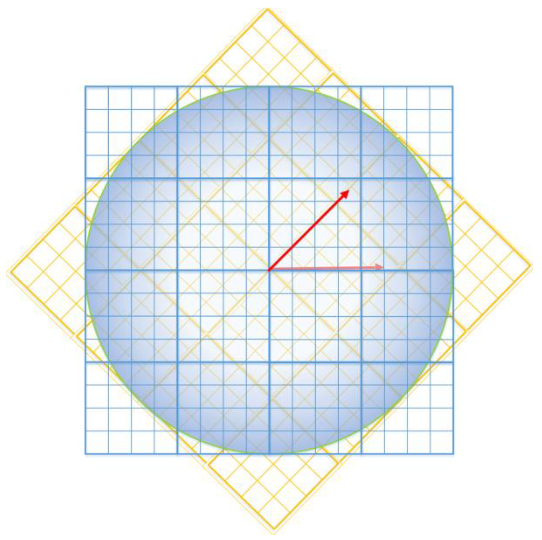
After obtaining the PAMI and the main phase angle, a 96 × 96 area is rotated with the feature point as the center, the angle of rotation is the main phase angle, and the rotated coordinates can be derived from the following equation:

$$\left[\begin{array}{c}{x}^{\prime }\\ y^{\prime }\end{array}\right]=\left[\begin{array}{cc}\cos \phi & -\sin \phi \\ \sin \phi & \cos \phi \end{array}\right]\left[\begin{array}{c}x\\ y\end{array}\right]$$

(21)

Because the rotated coordinates are not integer points, a quadratic interpolation is required to find the index value in PAMI corresponding to the rotated coordinates.

As shown in Figure 5, the red arrow indicates the phase angle counted, and this phase angle serves to be able to suppress rotational differences in the same region of different images; the blue grid region is the image coordinate information; the green circle indicates the extraction of the main phase angle region; and the yellow region is the post-rotation coordinate information. It can be observed that assuming that the rotation of the circular region of the 45° rotation will not result in the loss of the rotating, but the rotating coordinate points and the image coordinate points do not overlap, due to the image as an indexed value image, which cannot be directly estimated to be the nearest point, it is necessary to carry out a quadratic interpolation to calculate the index value corresponding to the coordinates of the change. The formula is as follows:

$$in{d}_x=(1-\mathrm{\Delta }y)\times (\mathrm{\Delta }x\times in{d}_{x_1}+(1-\mathrm{\Delta }x)\times in{d}_{x_0})+\mathrm{\Delta }y\times (\mathrm{\Delta }x\times in{d}_{x_3}+(1-\mathrm{\Delta }x)\times in{d}_{x_2})$$

(22)

In Equation (22), $in{d}_x$ denotes the corresponding index value in $(x,y)$ coordinates, $\mathrm{\Delta }y$ denotes the vertical coordinate $y-y_0$, and $\mathrm{\Delta }x$ denotes the horizontal coordinate $x-x_0$.

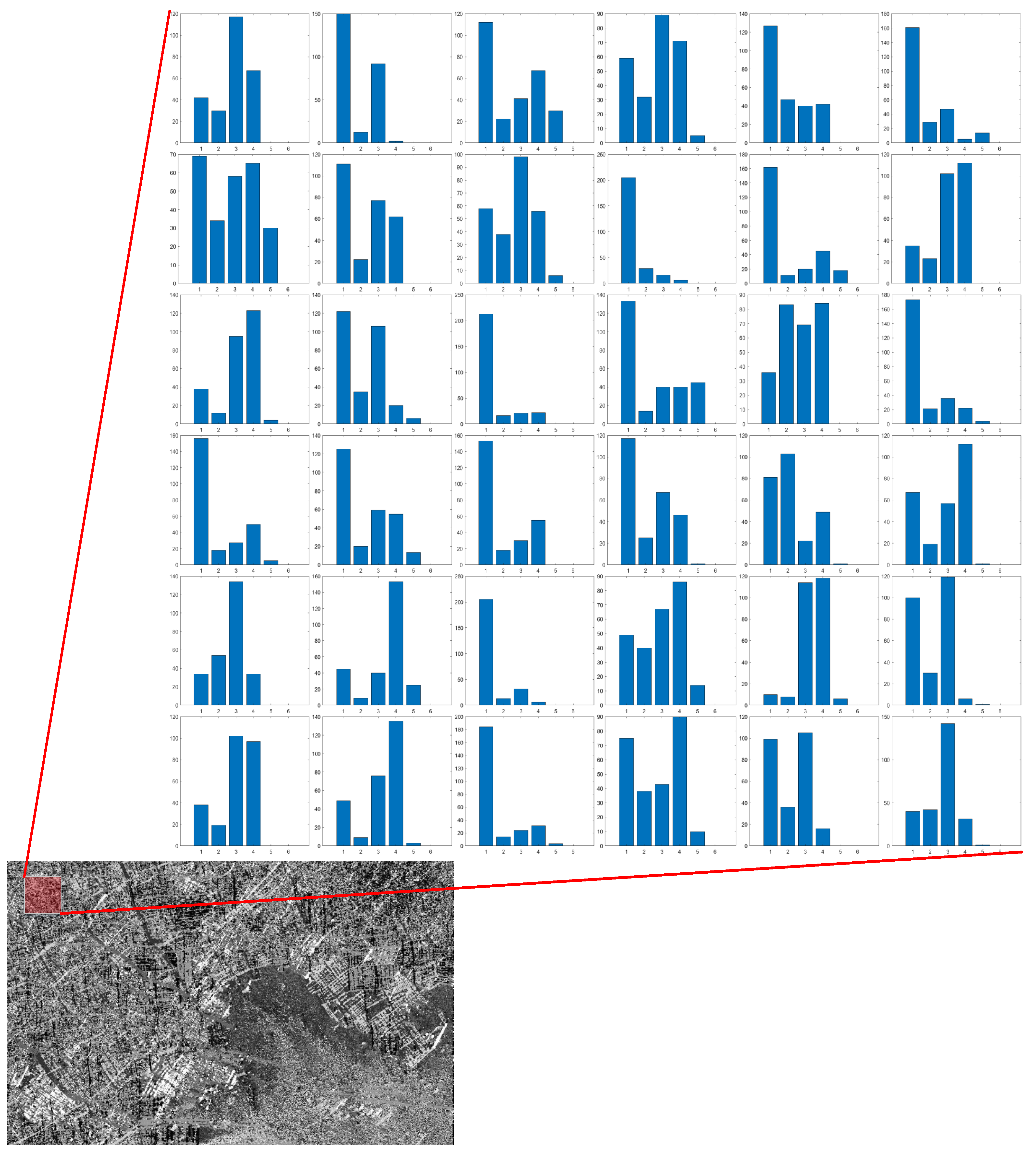
For this time, the region 96 × 96 is divided into 36 small regions of 16 × 16 and the histogram is used to count the number of indexes in each region, constituting 6 × 6 × 6 feature vectors.

Figure 6 shows that, to visualize the descriptors, we visualized the descriptors extracted from the area around a feature point (red), with the horizontal coordinates indicating the six directions and the vertical coordinates indicating the number of statistics, and each small histogram represents a PAMI statistic for a 16 × 16 area. Finally, the descriptors are normalized to increase the similarity between the descriptors, and finally, a 216-dimensional feature vector is formed.

4. Feature Matching and Outlier Removal

Feature matching is conducted by calculating the similarity between the feature vectors to derive the correspondence between the feature points. Here, the sum of squares of Euclidean distances (SSD) is used to measure the extracted feature vectors. Using the sum of squares of Euclidean distances (SSD), it is calculated as follows:

$$S={\displaystyle \sum _{i=1}^O{(D_r(x_r,y_r)-D_s(x_s,y_s))}^2}$$

(23)

In Equation (23), S is the SSD value of the PAMI feature vector $D_r(x_r,y_r)$ at the reference image feature point $(x_r,y_r)$ and the PAMI feature vector $D_s(x_s,y_s)$ at the image feature point $(x_{\mathrm{s}},y_{\mathrm{s}})$ to be aligned, and $O$ is the vector dimension.

For multi-source images, there may be a large number of mismatched points in the initial matching, and the mismatched points are called outer points, which are all over the feature point set and need to be eliminated to leave the stable inner points. Calculate the distance between all feature points between the reference image feature points and the feature points of the image to be aligned, set to C. Firstly, select the first M (M is 20 in the experiment) feature distance minimum points in C to form $C_{\mathrm{sample}}$. At this time, $C_{\mathrm{sample}}$ contains the matching relationship between the optimal feature points of the two images. Secondly, randomly select four feature points from M at a time to compute the affine matrix, and affine transform its corresponding matching points. The area ratio of the four triangles is formed by the four points, and if the area ratio changes, the correspondence is wrong. After traversing to find the feature points that can satisfy the constant area ratio (at least four), use C to count the number of internal points (the root mean square error of the computation of the feature points after the affine transformation and the corresponding reference image feature points is less than the threshold value of five, i.e., it is an internal point) in the current affine model, and the more internal points there are, the higher the confidence level of the current affine model is. Finally, the affine model with the highest confidence level is obtained after a continuous cycle.

5. Experiences

In this paper, the correct matching rate CMR, root mean square error RMSE, and running time are used to quantitatively evaluate the alignment results, respectively. The RMSE and CMR are calculated as follows:

$$RMSE=\sqrt{\frac{1}{N_c}{\displaystyle \sum _{i=1}^{N_c}\left[{\left(x_1^i-x_2^i\right)}^2+{\left(y_1^i-y_2^i\right)}^2\right]}}$$

(24)

$$CMR=\frac{N_c}{N}$$

(25)

In the equation, N is the number of matching pairs; $(x_1^i,y_1^i)$ and $(x_2^i,y_2^i)$ are the coordinates of matching point pairs; $(x_2^i,y_2^i)$ are the coordinates transformed by affine transformation matrix H; and $N_C$ is the number of correct matching pairs. It is stipulated that the distance between the points with the same name after affine transformation is less than five pixels, which is the correct match.

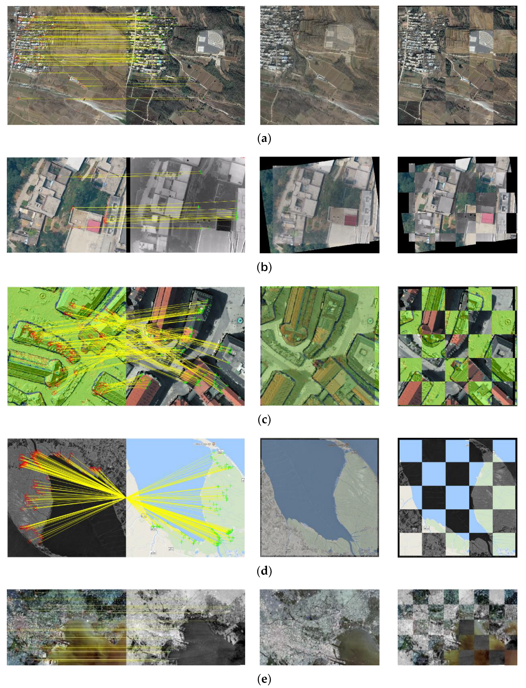
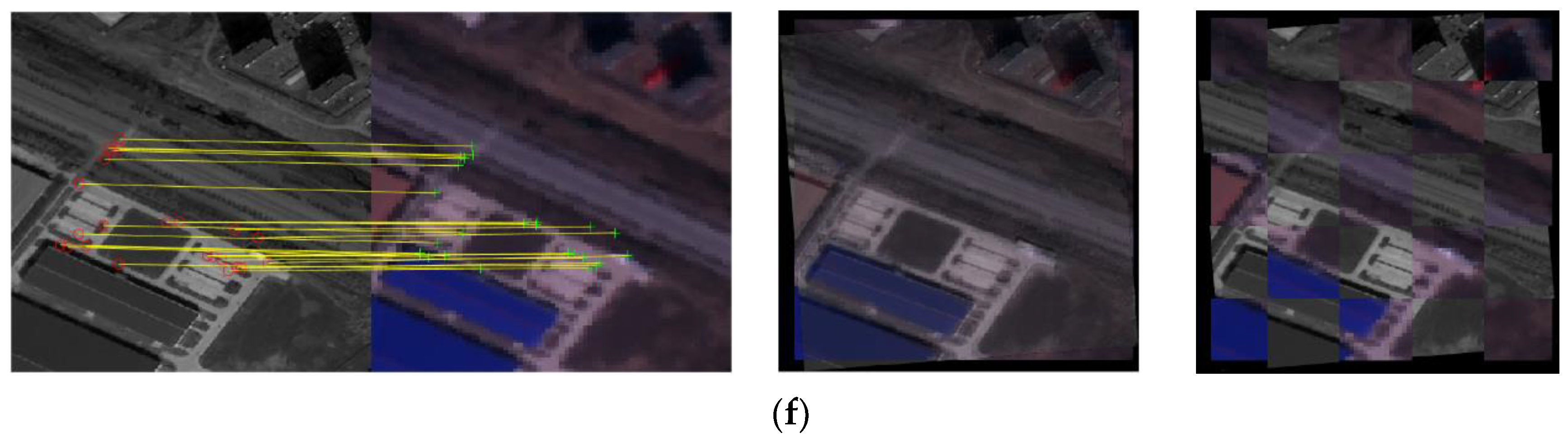
The data used in the experiments are multi-source image pairs of six scenes, labeled a to f, with both multi-sensor images and multi-temporal images of the same sensor, including hyperspectral images (HSI), multi-spectral (MSI), SAR, optical images, infrared images, depth maps, and rasterized maps (Map). These selected experimental data contain all the problems in multi-source image alignment, including large resolution differences, severe radiometric distortion, spatial distortion, rotation, content detail differences, and image noise. The alignment results of the gradient weakly sensitive alignment method for images in different scenarios are shown in Figure 7, where the red center point and the green center point are the stable feature points in the reference image and the image to be aligned, and the yellow line is the established match. From the alignment results, the method in this paper can overcome the problems in multi-source image alignment with strong robustness. The matching performance of the gradient weakly sensitive multi-source sensor alignment method can be adapted to a wide range of scenarios for the following reasons: (1) This method uses the maximum moment map instead of the image gradient edge map for feature detection, and takes into account the feature repetition rate and the number of features, which lays the foundation for subsequent matching. (2) The main phase angle is introduced to bypass the process of finding the gradient. The more accurate main phase angle is estimated in a certain interval by parabolic interpolation so that the final descriptor has rotational invariance. (3) This method constructs PAMI to convert heterogeneous images into homogeneous ones, which has good resistance to nonlinear radiation differences and ensures the robustness of this method.

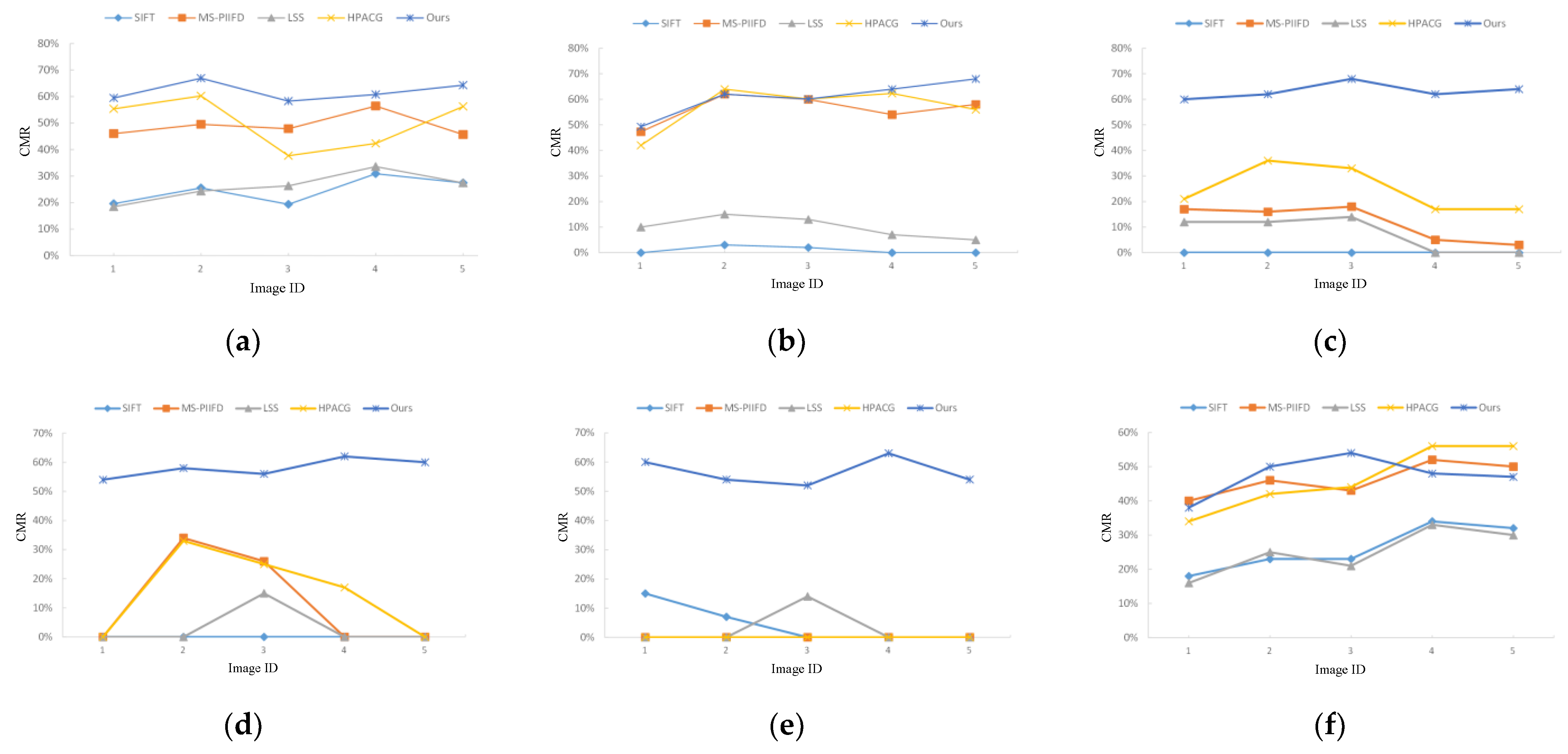
To qualitatively verify the effectiveness of the proposed gradient weakly sensitive alignment method, six groups of five different multi-source image data pairs each are used to test the robustness and generality of the proposed algorithm, and four multi-source alignment algorithms are selected for comparative CMR comparison, including SIFT, LSS, MS-PIIFD, and HPACG, which are not considered in the comparison because HOPC needs to provide the latitude/longitude information of the image disguised as a coarse alignment.

In Figure 8, five methods are shown in six sets of multimodal images CMR metric, and the smaller the difference in the imaging mechanism between images, the higher the correct rate of the response of the methods based on the gradient extraction of features, but the correct rate is difficult to be guaranteed if the image difference is large, such as SAR–optical, depth–optical, and map–optical. The method proposed in this paper does not involve the image gradient information, so it can maintain the strong robustness in multimodal images, especially in the existence of temporal differences between optical–optical, and can also maintain a high correct matching rate, and from the overall curve of the 1–5 group, there are no large fluctuations, which further indicates that the algorithm in this paper is robust. However, in the HSI–MSI group experiments in this paper, although the second and third trials obtained a high correct matching rate, large-scale differences can be seen from the subsequent experiments, due to the experimental image, so this paper’s algorithm detects fewer feature points.

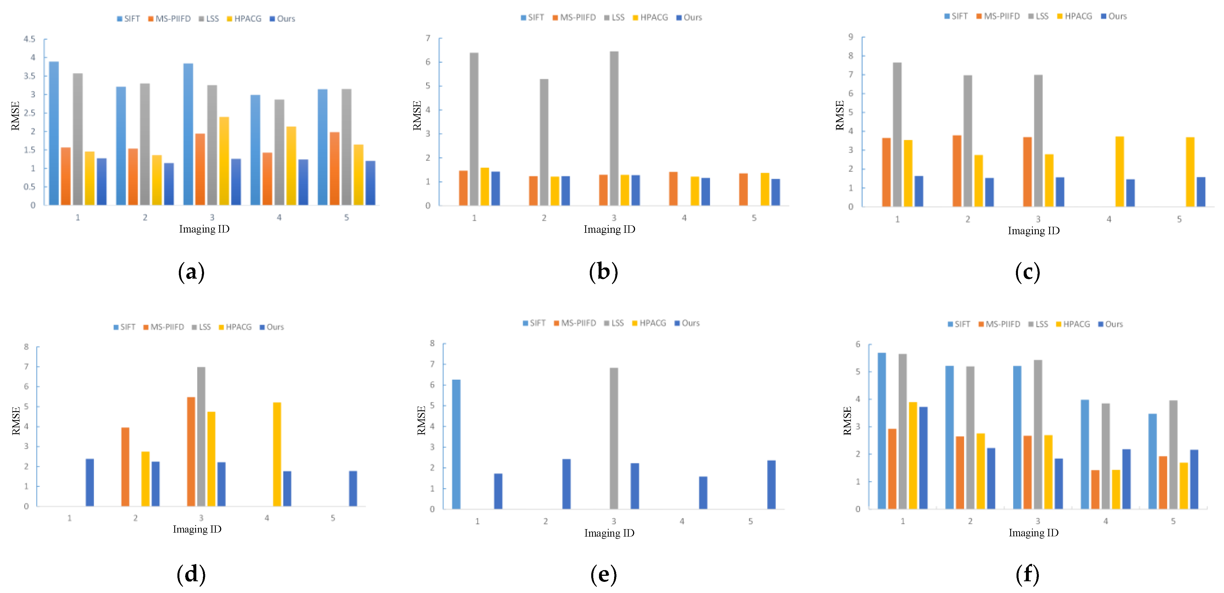
As shown in Figure 9, which shows the RMSE metrics of five methods in six sets of multimodal images, the corresponding RMSE values are not shown in the histograms because some of the alignment methods are not successfully aligned in the multi-source images so that the computed affine matrices will get a large RMSE value. From the RMSE values, it can be concluded that the algorithm in this paper not only has the advantage of robustness compared to other algorithms, but also has a high accuracy, especially to cope with the gradient reversal phenomena in images such as map–optical, depth–optical, and SAR–optical. From the optical–optical experiments, due to the existence of images 3, 4, and 5 in the experiments, there are some differences in the timing of the images. From Figure 7a, it can be seen that the timing differences lead to some scene changes, but this paper’s algorithm in the process of aligning such images did not lead to the root mean square error being too large because of the timing differences, from 1–5 as a whole, and compared with the current algorithm. This paper’s algorithm also has a stronger resistance to the timing differences.

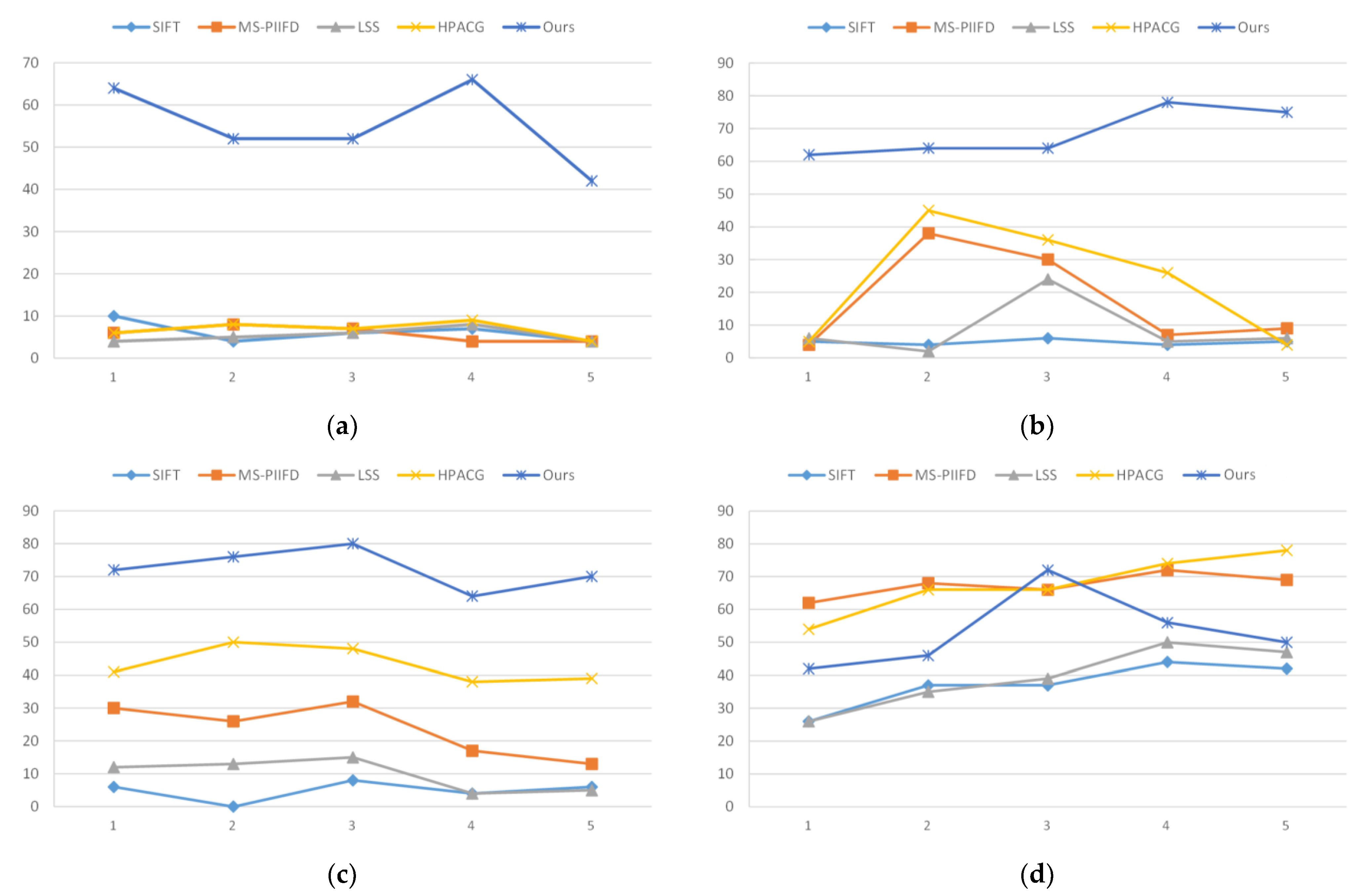
To visualize the robustness of this paper’s algorithm, we have quantitatively counted the number of correct matches for map–optical, depth–optical, SAR–optical, and HSI–MSI experimental groups $N_c$ as shown in Figure 10:

As shown in Figure 10, which shows the quantitative statistics of the five methods in four groups of multimodal image Nc, it can be seen from the map–optical, depth–optical, and SAR–optical groups of images that this paper’s algorithm can screen the largest number of correct matching points in the case of heterogeneous images, which ensures the robustness of the alignment algorithm. However, since the algorithm in this paper does not have strong scale invariance, the correct matching points screened in the face of the HSI–MSI group will be weaker than the current MS-PIIFD and HPACG algorithms. However, since the method in this paper is fundamentally a feature matching method, it will have excellent performance for images with not large-scale differences, such as three in HSI–MSI.

6. Conclusions

Aiming at the problem of heterogeneous remote sensing images, such as the existence of nonlinear intensity differences and other issues that lead to the difficulty of alignment, we propose a gradient weakly sensitive alignment method for multi-source sensor images. In this paper, the algorithm resists the nonlinear radiation differences between multi-source sensor images due to the use of the maximum moment map for feature point detection, uses the frequency domain information instead of the spatial domain information for feature detection, ensures the number of repetitive feature points between the images, and estimates the main phase angle by quadratic interpolation to estimate the phase angle in the 98 × 98 range near the feature points, thus making its algorithm rotationally invariant. Secondly, the conversion of heterogeneous images into isomorphic images increases the similarity between images and increases the SSD metric for feature descriptors to a certain extent in the feature matching stage, to establish more reliable alignment relationships. In the experimental stage, it is confirmed that the algorithm of this paper, regardless of the homogeneous images optical–optical with temporal differences, or SAR, depth, and map images with nonlinear radial differences, shows strong alignment robustness and accuracy. After qualitative and quantitative experiments, the algorithm in this paper achieves the most correct matching points and the most stable root mean square error as long as the experimental subjects do not have large-scale differences.

7. Foresight

Currently, in this paper, the algorithm solves the multimodal image alignment problem, but its qualitative and quantitative experimental verification, from the experimental results, still have some shortcomings, such as in the alignment of HSI. As some HSI images will have large-scale differences, if you seek to make the algorithm with scale invariance needs to be integrated into the scale invariance module, and the subsequent research will focus on processing, and based on the existing improvement, will ensure accuracy along with scale invariance.