Adaptive Backstepping Time Delay Control for Precision Positioning Stage with Unknown Hysteresis

Abstract

Piezoelectric-actuated precision positioning stages are widely used in high-precision instruments and high-end equipment due to their advantages of high resolution, fast response, and compact size. However, due to the strong nonlinearity of hysteresis, the presence of hysteresis in piezoelectric actuators seriously affects the positioning accuracy of the system. In addition, it is challenging to identify the model parameters for hysteresis. In this paper, an adaptive backstepping time delay control method is proposed for piezoelectric devices system with unknown hysteresis. Firstly, the Bouc–Wen model is used to describe the hysteresis characteristics, and the model is interpreted as a linear term and a bounded uncertain hysteresis term. Then, the time delay estimation technique is used to estimate the hysteresis term of the Bouc–Wen model online, and the unknown parameters of the system and hysteresis model are obtained through adaptive updating laws. Furthermore, the stability of the control scheme is proved based on Lyapunov stability theory. Finally, the effectiveness and superiority of the proposed control scheme are demonstrated by comparing it with two typical hysteresis compensation control algorithms through three different sets of input signals.

1. Introduction

Actuators and sensors made from smart materials (such as piezoelectric ceramics, magnetostriction, and shape memory alloys) are widely used in mechatronic systems like precision instruments and high-end equipment due to their high-resolution and fast-response characteristics. Applications include piezoelectric precision positioning mechanisms [1], atomic force microscopes [2], piezoelectric valves [3], and rapid tool servo systems [4]. However, the hysteresis present in smart materials often severely degrades the performance of mechatronic systems and can even lead to system instability [5]. Moreover, compared with traditional nonlinearities, the multivalued mapping [6], memory effects [5], and rate-dependency [7] make its modeling and control exceptionally challenging.Therefore, over the past thirty years, the problem of modeling hysteresis characteristics and their compensation control has attracted the attention of many scholars [8]. In the aspect of hysteresis modeling, there are currently three main methods. The first is the physical modeling approach, which includes the Jiles–Atherton model [9], Maxwell-slip model [10], etc.; the second is the phenomenological modeling approach, which includes the Bouc–Wen model [11], Preisach model [12], Prandtl–Ishlinskii model [13], etc.; the last one is the computational intelligence-based intelligent modeling approach, which mainly includes neural network models, fuzzy tree models [14], etc. Overall, although there are several modeling methods for hysteresis, due to its strong nonlinear characteristics, modeling and parameter identification remain challenging issues. Therefore, considering situations where the hysteresis parameters are unknown and designing appropriate controllers become important.

Based on the establishment of the hysteresis model, the compensation control of systems with hysteresis has gradually become a hot topic in the field of nonlinear control and has achieved a lot of results [15,16,17,18,19]. Roughly speaking, there are three main methods of hysteresis compensation control, one is feedforward compensation control, the second is feedback compensation control, and the last is feedback–feedforward compensation control.

Feedforward compensation control is a very effective and low-cost hysteresis compensation control method. After Krejci and Kuhnen [15] gave the analytical inverse of the classical Prandtl–Ishlinskii (P-I) model for the first time, it greatly promoted the popularization and application of this method. However, due to its open-loop mode, it depends entirely on the accuracy of the model and is sensitive to external disturbances and model uncertainties.

The feedback compensation control method does not need to construct a hysteresis inverse model or an approximate inverse model but treats the whole hysteresis or the nonlinear part of the hysteresis as a disturbance or an uncertainty. Therefore, the existing control theory and methods can be directly used to design feedback controllers. For example, Ikhouane [16] decomposed the Bouc–Wen hysteresis into a linear term and a nonlinear hysteresis term, and for the first time theoretically proved the boundedness of the Bouc–Wen nonlinear hysteresis term. This allows the nonlinear hysteresis term to be treated as a bounded disturbance, enabling the design of a feedback controller. Zhang [17] addressed a class of nonlinear systems with unknown hysteresis driving by treating the nonlinear term of Bouc–Wen hysteresis as a bounded disturbance and designed a hysteresis compensation controller using an adaptive approach. Zheng [18] proposed a high-gain feedback controller to eliminate the effects of hysteresis. A continuous high-order sliding mode controller was proposed to eliminate the hysteresis disturbance, and the closed-loop stability of the control system was proved theoretically [19]. In [20], hysteresis is decomposed into a linear term and a bounded nonlinear term, and then the bounded nonlinear term is estimated online by the adaptive controller. In [13], a continuous P-I hysteretic model is decomposed into a discrete P-I model and a small bounded error term. Then, an adaptive inverse is used to eliminate the effect of the discrete hysteresis, and the bounded error term is compensated by an online estimation technique. Although the feedback control method does not require the construction of a hysteresis inverse model, and treating the nonlinear hysteresis term merely as a disturbance, the design of the feedback controller cannot adopt excessively high gains to suppress these factors, especially when the hysteresis characteristic is particularly severe (for example, under high-frequency input, the hysteresis characteristic is significantly more severe than at low frequencies).

The feedback–feedforward compensation control method [21] is to construct an inverse model in the feedforward channel to eliminate the influence of hysteresis and design a controller in the feedback channel to further improve the performance of systems. Chen [22] proposed a pseudo-inverse algorithm to obtain the inverse model of P-I hysteresis to solve the difficulty of obtaining an analytical inversion and designed an adaptive feedback control to further improve the system performance. Fan [23] established a direct inverse of the rate-dependent P-I hysteresis model, and designed a PI controller with a disturbance observer, thus constructing a hybrid feedback–feedforward control algorithm to eliminate the effect of hysteresis. Although the feedback–feedforward control method can effectively improve the system bandwidth and control accuracy to a certain extent, the construction of the complex hysteresis inverse model itself is a difficult thing.

Time delay control [24] was first proposed in the 1990s. Its primary concept is to estimate the unknown dynamic characteristics and disturbances at the current moment by using information from a very short period (artificially introduced delay time) prior to the system’s state and its derivatives. In principle, as long as the delay time is sufficiently short and the unknown dynamic characteristics are continuous, the estimation error can be minimal and sometimes even negligible. Due to its clear principles and simple implementation, time delay control has been widely applied in the design of control systems for electric motors and industrial robots in recent years [25,26,27].

To sum up, how to solve the unknown parameters of the hysteresis model, and propose a compensation control method that does not require the construction of an inverse hysteresis model such that the control method is relatively easy to implement in engineering, is still an urgent problem to be solved in hysteresis compensation control research. This is also the starting point of this paper.

The Bouc–Wen model is a widely used hysteresis model, especially after [16] theoretically proved the boundedness of its nonlinear hysteresis term, which has increasingly drawn attention to its application in control systems. Focusing on a class of piezoelectric device electromechanical systems driven by unknown Bouc–Wen hysteresis, this paper proposes a novel hysteresis compensation feedback control strategy based on time delay estimation technology. This control method uses time delay estimation to online estimate the hysteresis nonlinearity of the Bouc–Wen model, while the estimation errors introduced by the time delay estimator are compensated through adaptive laws, thereby further improving the control performance of the system. Subsequently, based on the adaptive backstepping technique, the adaptive and control laws for the system and unknown hysteresis parameters are designed. Finally, simulation results are given to demonstrate the effectiveness of the proposed scheme.

The main contributions of this paper can be summarized as follows:

(1) The adaptive backstepping time delay control strategy proposed in this paper does not require the construction of a hysteresis inverse model compared to feedforward hysteresis compensation control and feedback–feedforward hysteresis control strategies; unlike [16], which treats the Bouc–Wen nonlinear hysteresis term as a disturbance, the control strategy presented here employs time delay estimation technology to online estimate the hysteresis nonlinearity and incorporates it into the controller design, rather than merely considering it a bounded disturbance.

(2) The controlled system and hysteresis parameters considered in this paper are unknown, and the controller design requires only one hysteresis parameter, thus making the control strategy widely applicable and simple to implement.

(3) A time delay estimator is used to estimate the nonlinear part of the complex hysteresis, which not only overcomes the difficulty of hysteresis compensation but also is easier to implement in practice compared with the hysteresis inverse compensation control schemes.

The rest of this paper is organized as follows. The problem to be tackled is stated, and the control objective is given in Section 2. In Section 3, the controller design process is given, and the semi-globally uniformly boundedness of the closed-loop system is proved. In Section 4, the simulation results are presented. Conclusions are finally provided in Section 5.

2. Problem Statement

Consider a class of electromechanical systems with hysteresis driving for piezoelectric devices as presented in [28,29]:

$$\begin{array}{c}\hfill \left\{\begin{array}{cc}& M\ddot{x}+D\dot{x}+Fx=w,\hfill \\ & w=H\left[u\right]\left(t\right)\hfill \end{array}\right.\end{array}$$

(1)

where x, $\dot{x}$, and $\ddot{x}$ represent the position, velocity, and acceleration, respectively; M, D, and F denote the mass, damping, and stiffness coefficients, respectively; u is the voltage applied to the piezoelectric actuator; and $H\left[u\right]\left(t\right)$ is the Bouc–Wen hysteresis, and its parameters are unknown. $H\left[u\right]\left(t\right)$ can be expressed as in [16]:

$$w=H\left[u\right]\left(t\right)=\mu \kappa u+(1-\mu )\kappa \vartheta ={\mu }_{1}u+{\mu }_2\vartheta$$

(2)

where $0<\mu <1$ represents the weighting factor, $\kappa$ is a parameter associated with the nonlinear pseudo-natural frequency, ${\mu }_1$ and ${\mu }_2$ are constants of the same sign, and $\vartheta$ can be expressed by a first-order differential equation [16] as follows:

$$\dot{\vartheta }=\dot{u}-\beta |\dot{u}{\left|\right|\vartheta |}^{n-1}\vartheta -\chi \dot{u}{\left|\vartheta \right|}^n$$

(3)

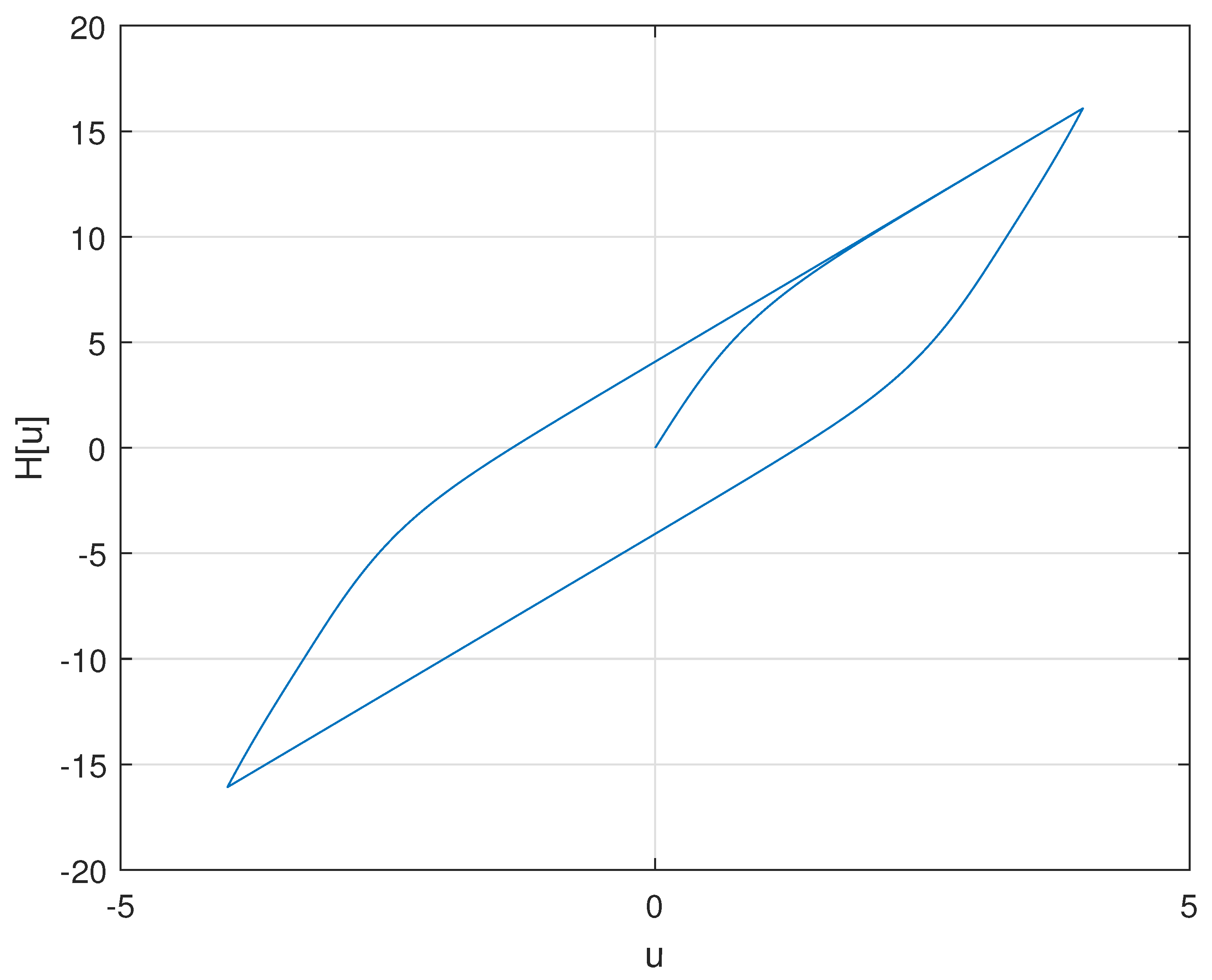
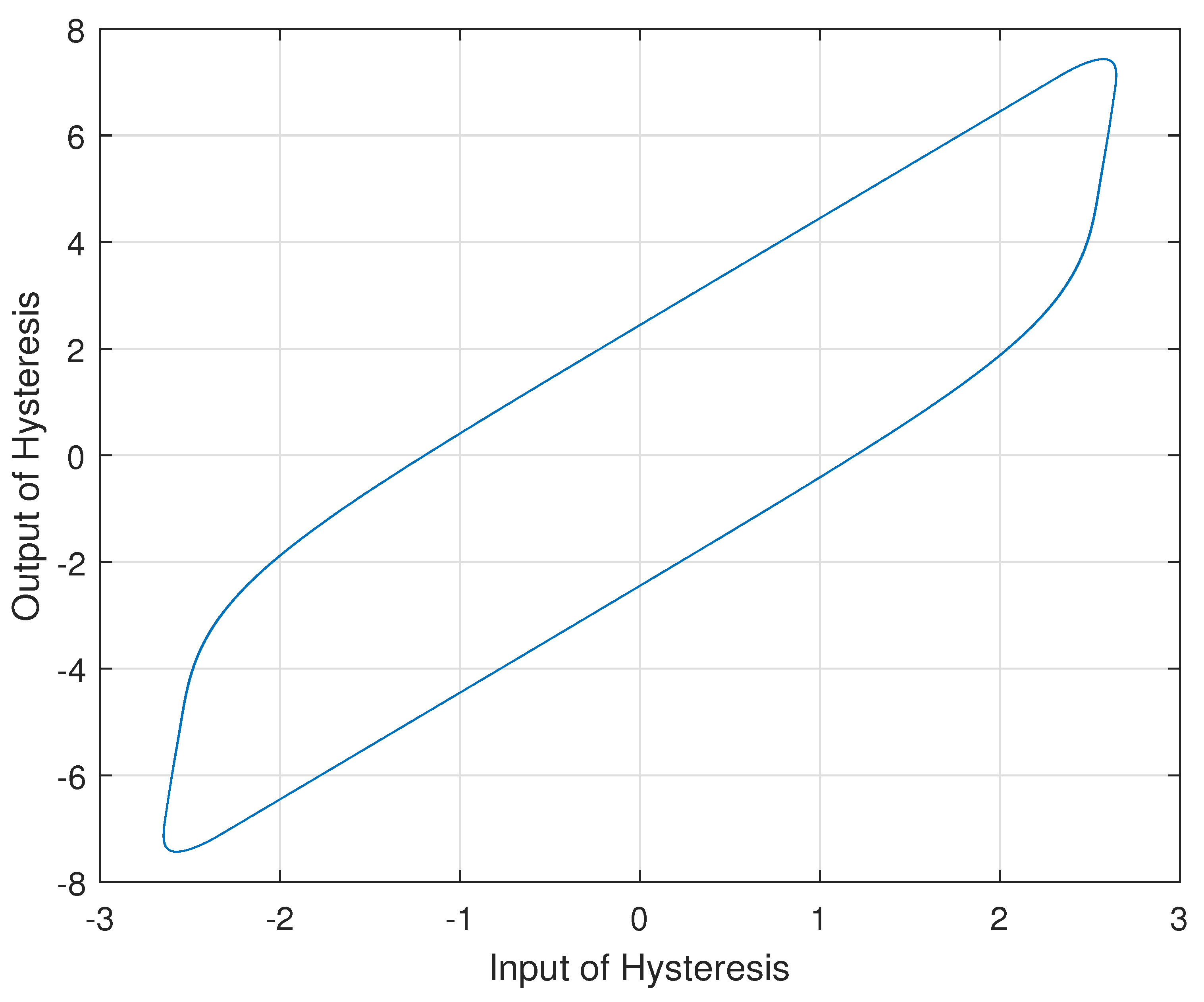
where $\beta$ and $\chi$ are parameters that describe the shape and magnitude of the hysteresis, respectively, while n is a parameter that controls the smoothness of the transition from the initial slope to the asymptotic slope. It is given that $\beta >x$ and $n>1$. When the parameters of the Bouc–Wen model are chosen as ${\mu }_1=3$, ${\mu }_2=5$, $n=2$, $\beta =1$, $\chi =0.5$, and the input signal is $u=4sin\left(2t\right)$, then the input–output relationship of the hysteresis is shown in Figure 1.

Below, two lemmas that will be used in subsequent controller designs are presented. These lemmas have been proven in [16,30], respectively.

Lemma 1 

([16]). For piecewise continuous signals u and $\dot{u}$ (bounded or unbounded), the solution $\vartheta \left(t\right)$ of Equation (3) is bounded, with the bound given by $\left|\vartheta \left(t\right)\right| \le max\left\{\right|\vartheta \left(0\right)|, \sqrt[n]{\frac{d{x}_1}{\beta +\chi }}\}$, where $\vartheta \left(0\right)$ is the initial value of ϑ.

Lemma 2 

([30]). For $\epsilon >0$ and $z\in R$, the following inequality holds:

$$0\le |z|-ztanh(\frac{z}{\epsilon })\le k\epsilon$$

(4)

where k is a constant that satisfies $k=e^{-(k+1)}$, that is, $k=0.2785$.

Remark 1. 

In general, the initial value of ϑ is taken as $\vartheta \left(0\right)=0$. According to Lemma 1, regardless of whether the input of the hysteresis is bounded or unbounded, $\vartheta \left(t\right)$ is bounded. Therefore, in the process of control design, the nonlinear term ${\mu }_2\vartheta$ of the Bouc–Wen hysteresis can be treated as a bounded disturbance, which is crucial for the controller design.

The design objective of the controller presented in this paper is to design appropriate adaptive laws and control laws such that the output displacement x of system (1) can track the desired trajectory $x_d$.

Assumption 1. 

In system (1), the velocity $\dot{x}$ is measurable.

Assumption 2. 

The desired trajectory $x_d$ and its first and second derivatives are known and bounded.

3. Controller Design

From Assumption 1, and by substituting Equation (2) into system (1), Equation (1) can be rewritten as:

$$\begin{array}{c}\hfill \left\{\begin{array}{cc}{\dot{x}}_1\hfill & =x_2,\hfill \\ M{\dot{x}}_2\hfill & ={\mu }_{1}u+\Gamma -D{x}_2-F{x}_1\hfill \end{array}\right.\end{array}$$

(5)

where $x_1=x$, $x_2=\dot{x}$, $\Gamma ={\mu }_2\vartheta$.

Based on the backstepping design methodology, the process of designing an adaptive backstepping time delay controller is as follows.

Step 1 Since the control objective is a tracking problem, we first define the generalized tracking error

$$\begin{array}{c}\hfill z_1=x_1-x_d.\end{array}$$

(6)

Then, taking the derivative of Equation (6), we obtain

$$\begin{array}{c}\hfill {\dot{z}}_1=x_2-{\dot{x}}_d.\end{array}$$

(7)

From (7), it is known that $x_2$ can be regarded as a virtual control input, and the virtual control law is designed as

$$\begin{array}{c}\hfill {\alpha }_1=-c_1{z}_1+{\dot{x}}_d\end{array}$$

(8)

where $c_1$ is a positive parameter to be designed. Next, we define the error variable

$$\begin{array}{c}\hfill z_2=x_2-{\alpha }_1.\end{array}$$

(9)

Therefore, from (6)–(9), we can derive:

$$z_1{\dot{z}}_1=-c_1{z}_1^2+z_1{z}_2.$$

(10)

Step 2 From (5)–(9), we have:

$$\begin{array}{ccc}\hfill M{\dot{z}}_2& =& M{\dot{x}}_2-M{\dot{\alpha }}_1\hfill \\ & =& {\mu }_{1}u+\Gamma -D{x}_2-F{x}_1-M{\dot{\alpha }}_1.\hfill \end{array}$$

(11)

The design of the adaptive backstepping time delay controller is as follows:

$$\begin{array}{c}\hfill \left\{\begin{array}{c}u=\widehat{\xi }{\alpha }_2\hfill \\ {\alpha }_2=-z_1-c_2{z}_2-\widehat{\Gamma }+\widehat{D}{x}_2+\widehat{F}{x}_1+\widehat{M}{\dot{\alpha }}_1-\widehat{B}tanh\left(\frac{z_2}{\epsilon }\right)\hfill \end{array}\right.\end{array}$$

(12)

where $c_2$ is a positive parameter to be designed, and $\widehat{\xi }$, $\widehat{\Gamma }$, $\widehat{D}$, $\widehat{F}$, and $\widehat{M}$ are estimates of parameters $\frac{1}{{\mu }_1}$, $\Gamma$, D, F, and M, respectively. $\widehat{B}$ is an estimate of the bound of the time delay estimation error. And the bound of the time delay estimation error B will be introduced below.

In the design of the controller, unlike traditional feedback hysteresis compensation methods that treat the nonlinear term $u_2\vartheta$ of the Bouc–Wen hysteresis as a bounded disturbance, this paper employs time delay estimation techniques to online estimate the nonlinear term of the hysteresis. Therefore, according to the principle of time delay estimation, from Equations (1) and (5), we obtain:

$$\begin{array}{ccc}\hfill \widehat{\Gamma }\left(t\right)& =& \Gamma (t-h)\hfill \\ & =& {\mu }_2{\vartheta }_2(t-h)\hfill \\ & =& M{\dot{x}}_2(t-h)+D{x}_2(t-h)+F{x}_1(t-h)-{\mu }_{1}u(t-h)\hfill \\ & =& w(t-h)-{\mu }_{1}u(t-h)\hfill \end{array}$$

(13)

where h represents a sufficiently small delay time. In practical implementation, h is generally set to the unit sampling time. It should be noted that both $\Gamma$ and $\widehat{\Gamma }$ are functions of time; they were not explicitly identified earlier for the sake of convenience and to maintain a consistent style in the formulas. Where it would not lead to confusion, we have often dropped the time argument (t) of variables. According to the principle of time delay control, as long as h is sufficiently small, it follows that $\Gamma \left(t\right)\cong \Gamma (t-h)=\widehat{\Gamma }\left(t\right)$. However, unless h is taken to be zero, there usually exists a time delay estimation error:

$$\begin{array}{c}\hfill e_d\left(t\right)=\Gamma \left(t\right)-\widehat{\Gamma }\left(t\right).\end{array}$$

(14)

Therefore, we use B to represent the bound of the time delay estimation error, that is, $|e_d\left(t\right)|\le B$.

Remark 2. 

According to Assumption 2, the desired state $x_d$ and its first and second derivatives are known and bounded. This implies that the variables $z_1$ and $z_2$, which are typically used in backstepping control system design, are also known and bounded. This is a prerequisite for the successful design of the virtual controller and the overall control system.

Remark 3. 

From Lemma 1, we know that ${\mu }_2{\vartheta }_2(t-h)$ is bounded; thus, it is reasonable for us to assume that the time delay estimation error is bounded. Moreover, in practical execution, by taking h as the unit sampling time, all values of the system from the previous sampling time are known. Therefore, from (13), the time delay estimation $\widehat{\Gamma }$ can be calculated using the following method: if w is measurable, then

$$\begin{array}{c}\hfill \widehat{\Gamma }\left(t\right)=w(t-1)-\frac{1}{\widehat{\xi }}u(t-1).\end{array}$$

(15)

Otherwise, it can be calculated by the following equation:

$$\begin{array}{ccc}\hfill \widehat{\Gamma }\left(t\right)& =& \widehat{M}{\dot{x}}_2(t-1)+\widehat{D}{x}_2(t-1)+\widehat{F}{x}_1(t-1)-\frac{1}{\widehat{\xi }}u(t-1).\hfill \end{array}$$

(16)

The adaptive update law for the parameters is designed as follows:

$$\begin{array}{c}\hfill \dot{\widehat{\xi }}=-{\gamma }_{\xi }(z_2{\alpha }_2+{\sigma }_{\xi }\widehat{\xi })\end{array}$$

(17)

$$\begin{array}{c}\hfill \dot{\widehat{D}}=-{\gamma }_D(z_2{x}_2+{\sigma }_D\widehat{D})\end{array}$$

(18)

$$\begin{array}{c}\hfill \dot{\widehat{F}}=-{\gamma }_F(z_2{x}_1+{\sigma }_F\widehat{F})\end{array}$$

(19)

$$\begin{array}{c}\hfill \dot{\widehat{M}}=-{\gamma }_M(z_2{\dot{\alpha }}_1+{\sigma }_M\widehat{M})\end{array}$$

(20)

$$\begin{array}{c}\hfill \dot{\widehat{B}}={\gamma }_B(z_{2}tanh\left(\frac{z_2}{\epsilon }\right)-{\sigma }_B\widehat{B})\end{array}$$

(21)

where $\tilde{\xi } = \xi -\widehat{\xi }$, $\tilde{D} = D-\widehat{D}$, $\tilde{F} = F-\widehat{F}$, $\tilde{M} = M-\widehat{M}$, $\tilde{B} = B-\widehat{B}$, and ${\gamma }_{\xi }$, ${\gamma }_D$, ${\gamma }_F$, ${\gamma }_M$, ${\gamma }_B$, ${\sigma }_{\xi }$, ${\sigma }_D$, ${\sigma }_F$, ${\sigma }_M$ and ${\sigma }_B$ are positive parameters to be designed.

We select the following Lyapunov function:

$$\begin{array}{ccc}\hfill V& =& \frac{1}{2}{z}_1^2+\frac{1}{2}M{z}_2^2+\frac{{\mu }_1}{2{\gamma }_{\xi }}{\tilde{\xi }}^2+\frac{1}{2{\gamma }_D}{\tilde{D}}^2+\frac{1}{2{\gamma }_F}{\tilde{F}}^2+\frac{1}{2{\gamma }_M}{\tilde{M}}^2+\frac{1}{2{\gamma }_B}{\tilde{B}}^2.\hfill \end{array}$$

(22)

Taking the time derivative of V and using Equations (10) and (11), we obtain

$$\begin{array}{ccc}\hfill \dot{V}& =& -c_1{z}_1^2+z_1{z}_2+z_{2}M{\dot{z}}_2-\frac{{\mu }_1}{{\gamma }_{\xi }}\tilde{\xi }\dot{\widehat{\xi }}-\frac{1}{{\gamma }_D}\tilde{D}\dot{\widehat{D}}\hfill \\ & & -\frac{1}{{\gamma }_F}\tilde{F}\dot{\widehat{F}}-\frac{1}{{\gamma }_M}\tilde{M}\dot{\widehat{M}}-\frac{1}{{\gamma }_B}\tilde{B}\dot{\widehat{B}}\hfill \\ & =& -c_1{z}_1^2+z_1{z}_2+z_2({\mu }_{1}u+\widehat{\Gamma }+e_d-D{x}_2\hfill \\ & & -F{x}_1-M{\dot{\alpha }}_1)-\frac{{\mu }_1}{{\gamma }_{\xi }}\tilde{\xi }\dot{\widehat{\xi }}-\frac{1}{{\gamma }_D}\tilde{D}\dot{\widehat{D}}\hfill \\ & & -\frac{1}{{\gamma }_F}\tilde{F}\dot{\widehat{F}}-\frac{1}{{\gamma }_M}\tilde{M}\dot{\widehat{M}}-\frac{1}{{\gamma }_B}\tilde{B}\dot{\widehat{B}}.\hfill \end{array}$$

(23)

Note the following fact:

$$\begin{array}{ccc}\hfill {\mu }_{1}u& =& {\mu }_1\widehat{\xi }{\alpha }_2={\alpha }_2-{\mu }_1\tilde{\xi }{\alpha }_2\hfill \\ \hfill z_2{e}_d& \le & |z_2|B.\hfill \end{array}$$

Substituting (12) into (23), we have

$$\begin{array}{ccc}\hfill \dot{V}& =& -c_1{z}_1^2-c_2{z}_2^2+z_2[-\tilde{D}{x}_2-\tilde{F}{x}_1-\tilde{M}{\dot{\alpha }}_1]\hfill \\ & & +|z_2|B-z_2\widehat{B}tanh\left(\frac{z_2}{\epsilon }\right)-z_2{\mu }_1\tilde{\xi }{\alpha }_2-\frac{{\mu }_1}{{\gamma }_{\xi }}\tilde{\xi }\dot{\widehat{\xi }}\hfill \\ & & -\frac{1}{{\gamma }_D}\tilde{D}\dot{\widehat{D}}-\frac{1}{{\gamma }_F}\tilde{F}\dot{\widehat{F}}-\frac{1}{{\gamma }_M}\tilde{M}\dot{\widehat{M}}-\frac{1}{{\gamma }_B}\tilde{B}\dot{\widehat{B}}\hfill \end{array}$$

(24)

Substituting (17)–(21) into (24), we obtain

$$\begin{array}{ccc}\hfill \dot{V}& =& -c_1{z}_1^2-c_2{z}_2^2+\left|z_2\right|B-z_{2}Btanh\left(\frac{z_2}{\epsilon }\right)\hfill \\ & & +{\sigma }_{\xi }\tilde{\xi }\widehat{\xi }+{\sigma }_D\tilde{D}\widehat{D}+{\sigma }_F\tilde{F}\widehat{F}\hfill \\ & & +{\sigma }_M\tilde{M}\widehat{M}+{\sigma }_B\tilde{B}\widehat{B}\hfill \end{array}$$

(25)

Note that

$$\begin{array}{cc}& \tilde{D}\widehat{D}=\tilde{D}(D-\tilde{D})=\tilde{D}D-{\tilde{D}}^2\\ & \tilde{D}D\le \frac{1}{2}{\tilde{D}}^2+\frac{1}{2}{F}^2\end{array}$$

Therefore, the following inequality holds:

$$\begin{array}{c}\hfill \tilde{D}\widehat{D}\le -\frac{1}{2}{\tilde{D}}^2+\frac{1}{2}{D}^2\end{array}$$

(26)

Similarly, we have

$$\begin{array}{ccc}\hfill \tilde{F}\widehat{F}& \le & -\frac{1}{2}{\tilde{F}}^2+\frac{1}{2}{F}^2\hfill \end{array}$$

(27)

$$\begin{array}{ccc}\hfill \tilde{M}\widehat{M}& \le & -\frac{1}{2}{\tilde{M}}^2+\frac{1}{2}{M}^2\hfill \end{array}$$

(28)

$$\begin{array}{ccc}\hfill \tilde{B}\widehat{B}& \le & -\frac{1}{2}{\tilde{B}}^2+\frac{1}{2}{B}^2\hfill \end{array}$$

(29)

$$\begin{array}{ccc}\hfill \tilde{\xi }\widehat{\xi }& \le & -\frac{1}{2}{\tilde{\xi }}^2+\frac{1}{2}{\xi }^2\hfill \end{array}$$

(30)

Applying Lemma 2 to (24) and substituting (4), (16)–(30) into (25), we obtain

$$\begin{array}{ccc}\dot{V}\hfill & \le \hfill & -c_1{z}_1^2-c_2{z}_2^2-\frac{1}{2}{\tilde{\xi }}^2-\frac{1}{2}{\tilde{D}}^2-\frac{1}{2}{\tilde{F}}^2-\frac{1}{2}{\tilde{M}}^2\hfill \\ & & -\frac{1}{2}{\tilde{B}}^2+0.2785B\epsilon +\frac{1}{2}{\xi }^2+\frac{1}{2}{D}^2+\frac{1}{2}{F}^2\hfill \\ & & +\frac{1}{2}{M}^2+\frac{1}{2}{B}^2\hfill \\ & \le & -cV+\zeta \hfill \end{array}$$

(31)

where

$$\begin{array}{ccc}\hfill c& =& min(2c_1,2c_2,\frac{{\gamma }_{\xi }}{{\mu }_1},{\gamma }_D,{\gamma }_F,{\gamma }_M,{\gamma }_B)\hfill \\ \hfill \zeta & =& 0.2785B\epsilon +\frac{1}{2}{\xi }^2+\frac{1}{2}{D}^2+\frac{1}{2}{F}^2\hfill \end{array}$$

(32)

$$\begin{array}{ccc}& & +\frac{1}{2}{M}^2+\frac{1}{2}{B}^2.\hfill \end{array}$$

(33)

Theorem 1.  

For system (1), where the hysteresis model is described by (2) and (3), under the Assumptions 1 and 2, the adaptive backstepping time delay controller composed of the control law (8) and (12), the adaptive update laws (17)–(21), and the time delay estimate (13) can ensure that the closed-loop system is semi-globally uniformly bounded, all signals in the closed-loop system are bounded, and the system tracking error z asymptotically converges to the following compact set:

$$\begin{array}{c}\hfill \Omega :=\{z_1\in R|\left|z_1\right|\le \sqrt{Z}\}\end{array}$$

(34)

where $Z=2(V\left(0\right)+\frac{\zeta }{c})$, with c, ζ are given by (32) and (33).

The proof of this theorem is as follows. From Equation (31), we know that the closed-loop system is semi-globally uniformly bounded, and the signals $z_1$, $z_2$, $\tilde{\xi },\tilde{D},\tilde{F},\tilde{M}$, and $\tilde{B}$ are bounded. Therefore, the estimated signals $\widehat{\xi },\widehat{D},\widehat{F},\widehat{M},\widehat{B}$ are also bounded. Based on Assumption 1 and Equation (5), the states $x_1$, $x_2$ are similarly bounded. Further, from Equations (8) and (12), we can see that ${\alpha }_1$ and ${\alpha }_2$ are also bounded.

Next, we prove the convergence domain of $z_1$. By multiplying both sides of Equation (31) by $e^{ct}$, we have:

$$\begin{array}{c}\hfill \dot{V}{e}^{ct}\le -cV{e}^{ct}+\zeta e^{ct}.\end{array}$$

(35)

According to (35), we obtain

$$\begin{array}{c}\hfill \frac{d}{dt}\left(V{e}^{ct}\right)\le \zeta e^{ct}.\end{array}$$

(36)

By integrating Equation (36), we obtain

$$\begin{array}{c}\hfill V\le (V\left(0\right)-\frac{\zeta }{c})e^{-ct}+\frac{\zeta }{c}\le V\left(0\right)+\frac{\zeta }{c}.\end{array}$$

(37)

Regarding $z_1$, it holds that

$$\begin{array}{c}\hfill \frac{1}{2}{z}_1^2\le V\left(0\right)+\frac{\zeta }{c}.\end{array}$$

(38)

Therefore, from (38), we can derive

$$\begin{array}{c}\hfill |z_1|\le \sqrt{Z}.\end{array}$$

(39)

where $Z=2(V\left(0\right)+\frac{\zeta }{c})$. With this, the proof of Theorem 1 is complete.

Remark 4.  

Regarding the issue of parameter design in controllers, the following rules can be followed: (1) The constants $c_1$ and $c_2$ in the virtual controllers can enhance the system’s static performance, but excessively large values may cause system oscillation. It is necessary to make a reasonable choice and strike a balance between static and dynamic performance as in [31]. (2) As with other adaptive backstepping controls, the parameters in the adaptive update law (17)–(21) are generally designed to be small. (3) For the time delay estimator (13), the smaller the value of h, the better. In practical engineering, it is usually set to the sampling period of the control system.

4. Simulation Study

For the system shown in (1)–(3), the following nominal system parameters are chosen: $D=0.15\mathrm{Ns}/\mathrm{m}, M=1\mathrm{Kg}, F=1\mathrm{M}/\mathrm{m}$, ${\mu }_1=2$, ${\mu }_2=3$, $n=2$, $\beta =1$, $\chi =0.5$. The initial state of the system is $x\left(0\right)=0.6$. The desired trajectory for the control objective is $x_{d1}=5sin\left(0.5\pi t\right)$. This simulation is conducted in a Matlab environment, with the control law and adaptive update law parameters chosen as follows: $c_1=18$, $c_2=12$, ${\gamma }_{\xi }=0.02$, ${\gamma }_D=0.02$, ${\gamma }_F=0.02$, ${\gamma }_M=0.02$, ${\gamma }_B=0.015$, ${\sigma }_{\xi }=0.0049$, ${\sigma }_D=0.01$, ${\sigma }_F=0.01$, ${\sigma }_M=0.01$, ${\sigma }_B=0.01$, $\epsilon =0.01$. The initial states for the update law parameters are $\xi \left(0\right)=0.55$, $D\left(0\right)=0.2$, $F\left(0\right)=1.2$, $M\left(0\right)=0.8$, and $B\left(0\right)=1$. The estimated time delay for the time delay estimate is $h=0.001$.

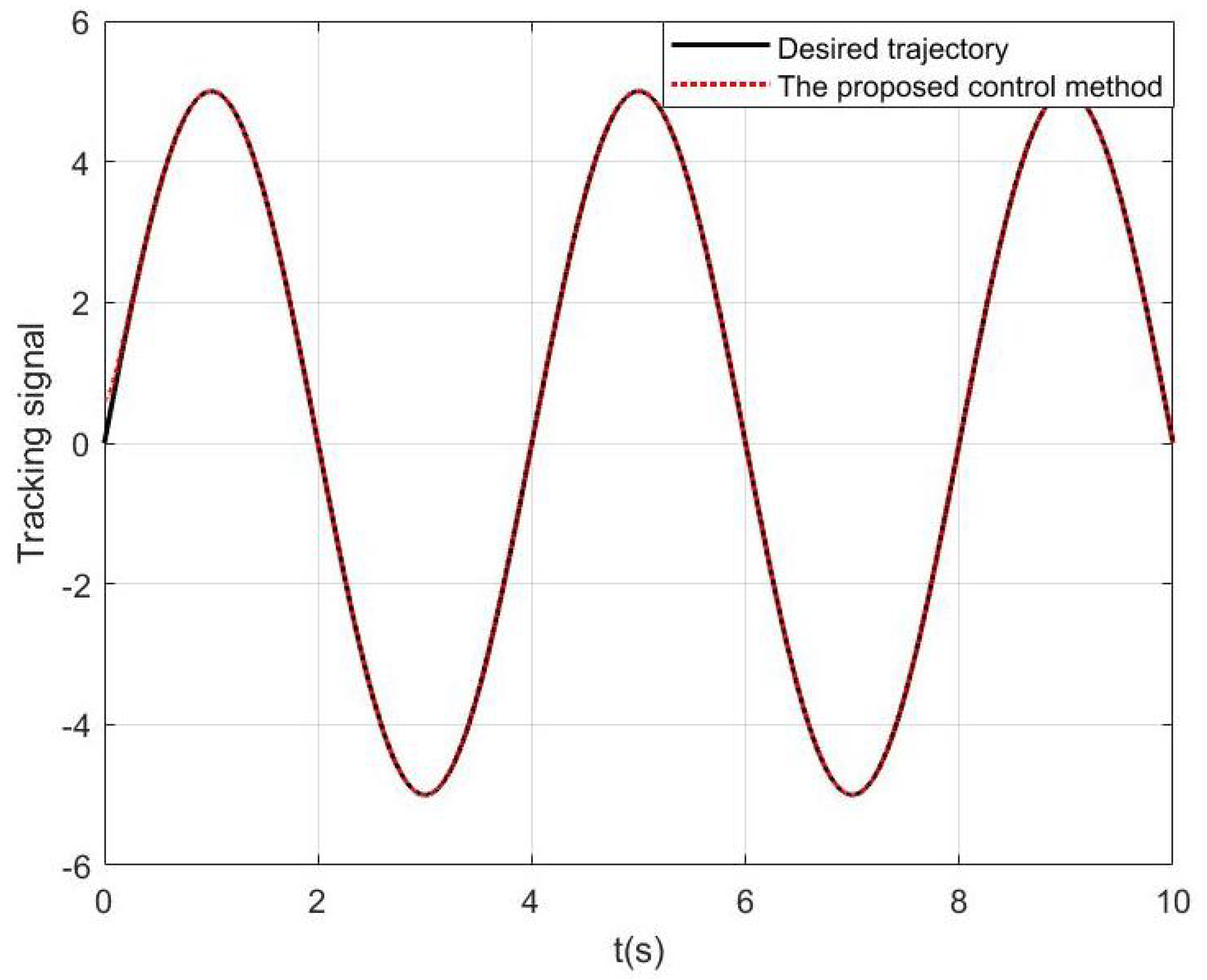
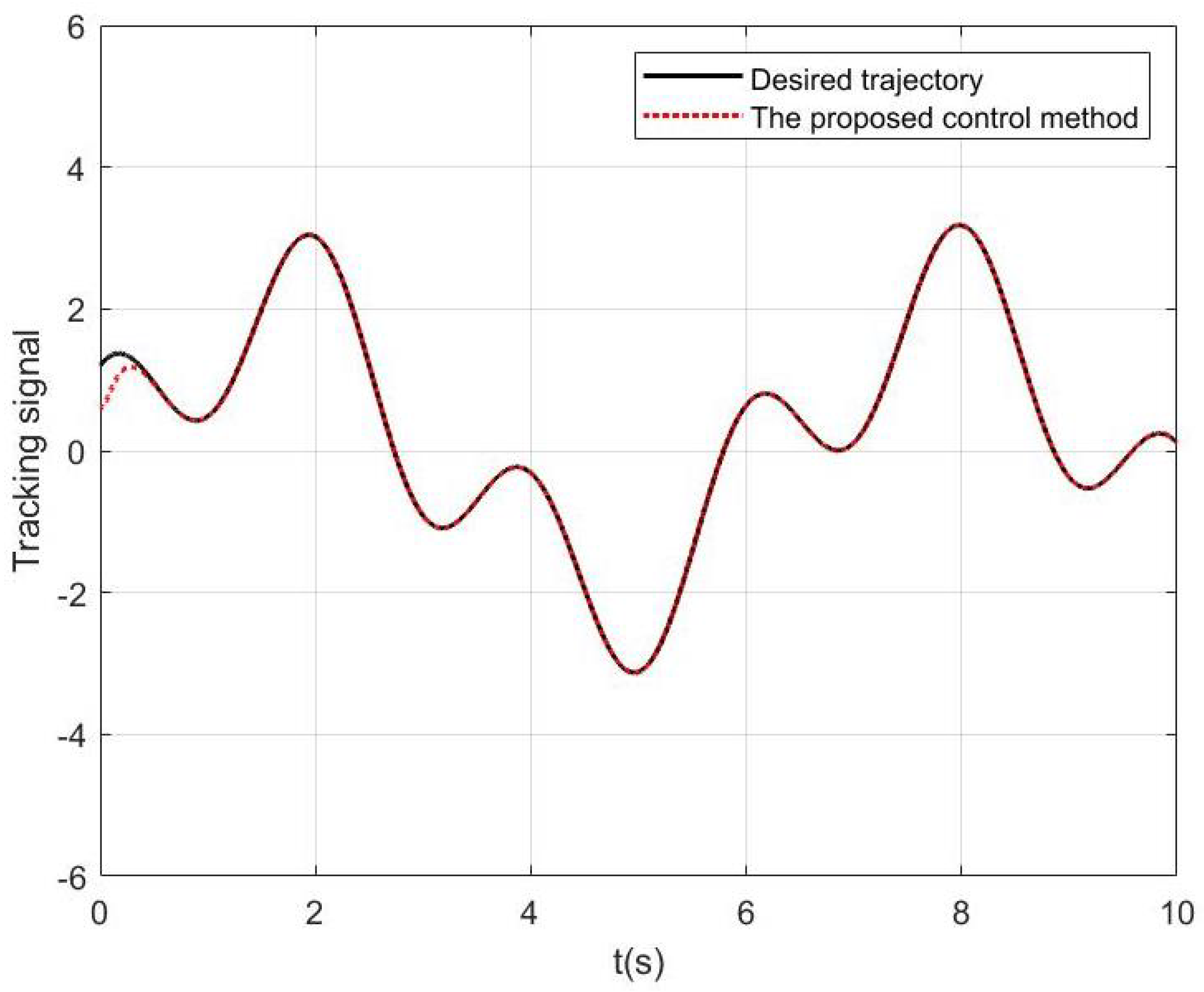
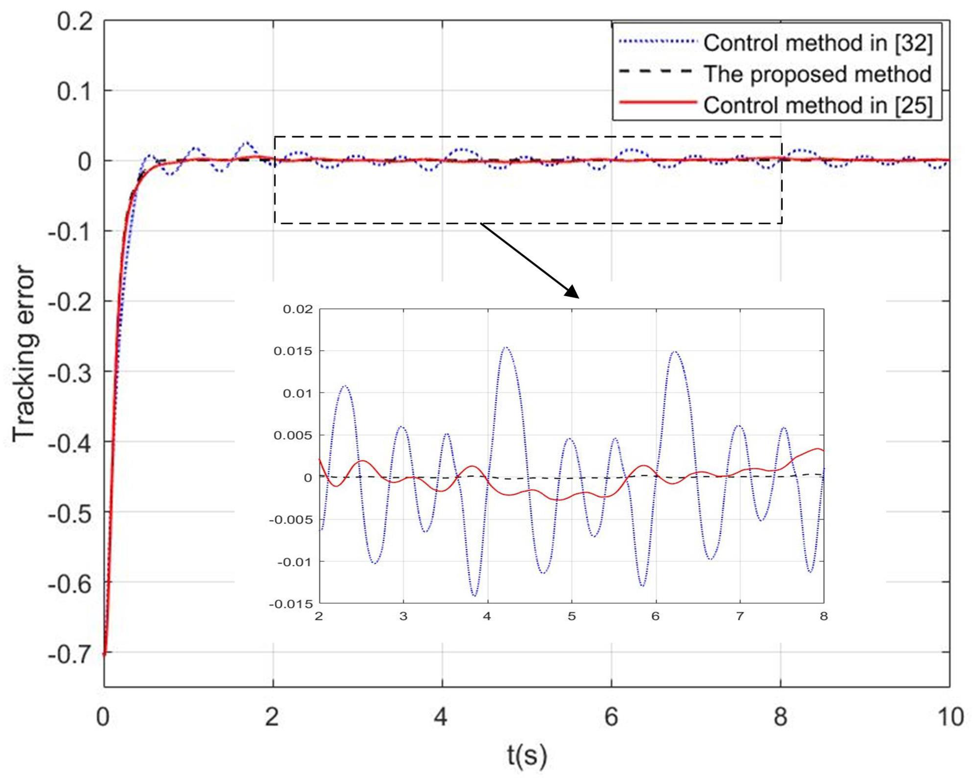
To demonstrate the effectiveness of the proposed control strategy, a comparison is made between the method presented in this paper and time delay-control-based control methods [25], as well as traditional hysteresis compensation control methods [32]. As shown in Figure 2, the system output tracking performance of the algorithm proposed in this paper is given. Clearly, the system’s output can track the desired trajectory well. 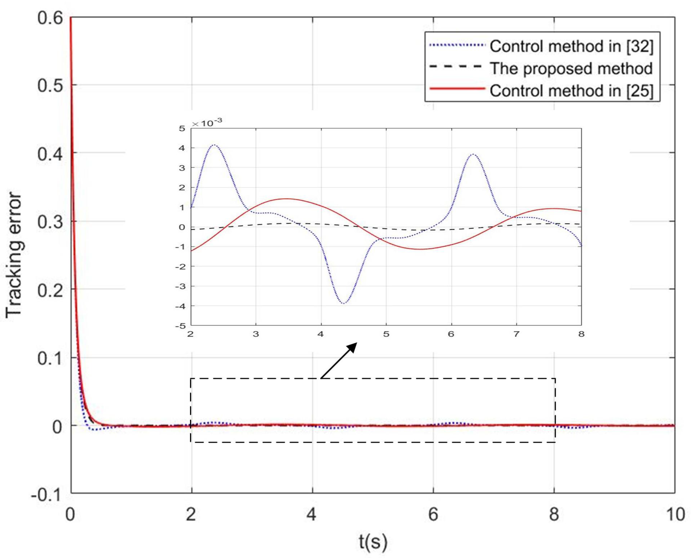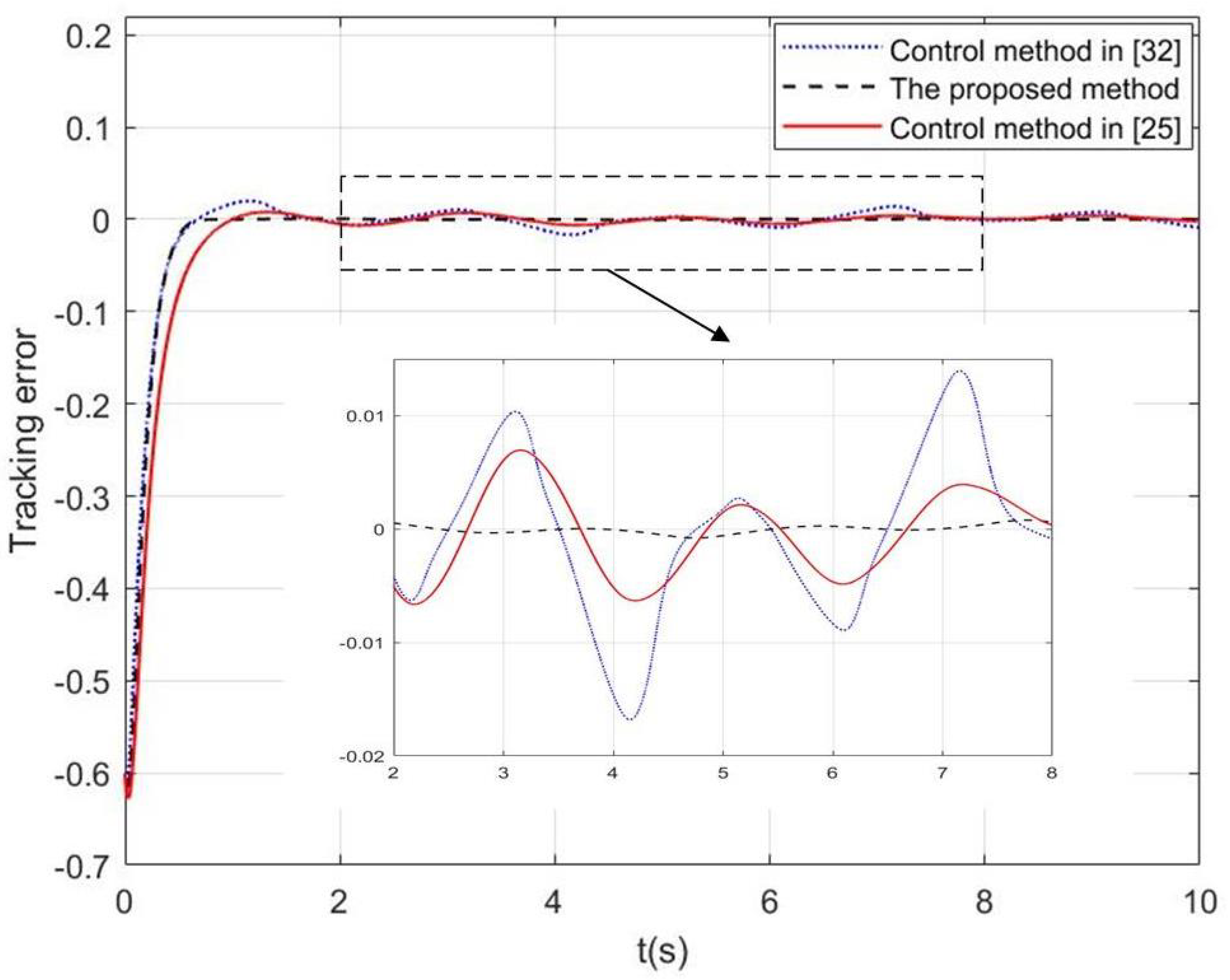From Figure 3, it can be seen that the control method proposed in this paper has a smaller tracking error compared to the other two control methods. This demonstrates the superiority of the proposed control method in reducing tracking errors, thereby proving its effectiveness. 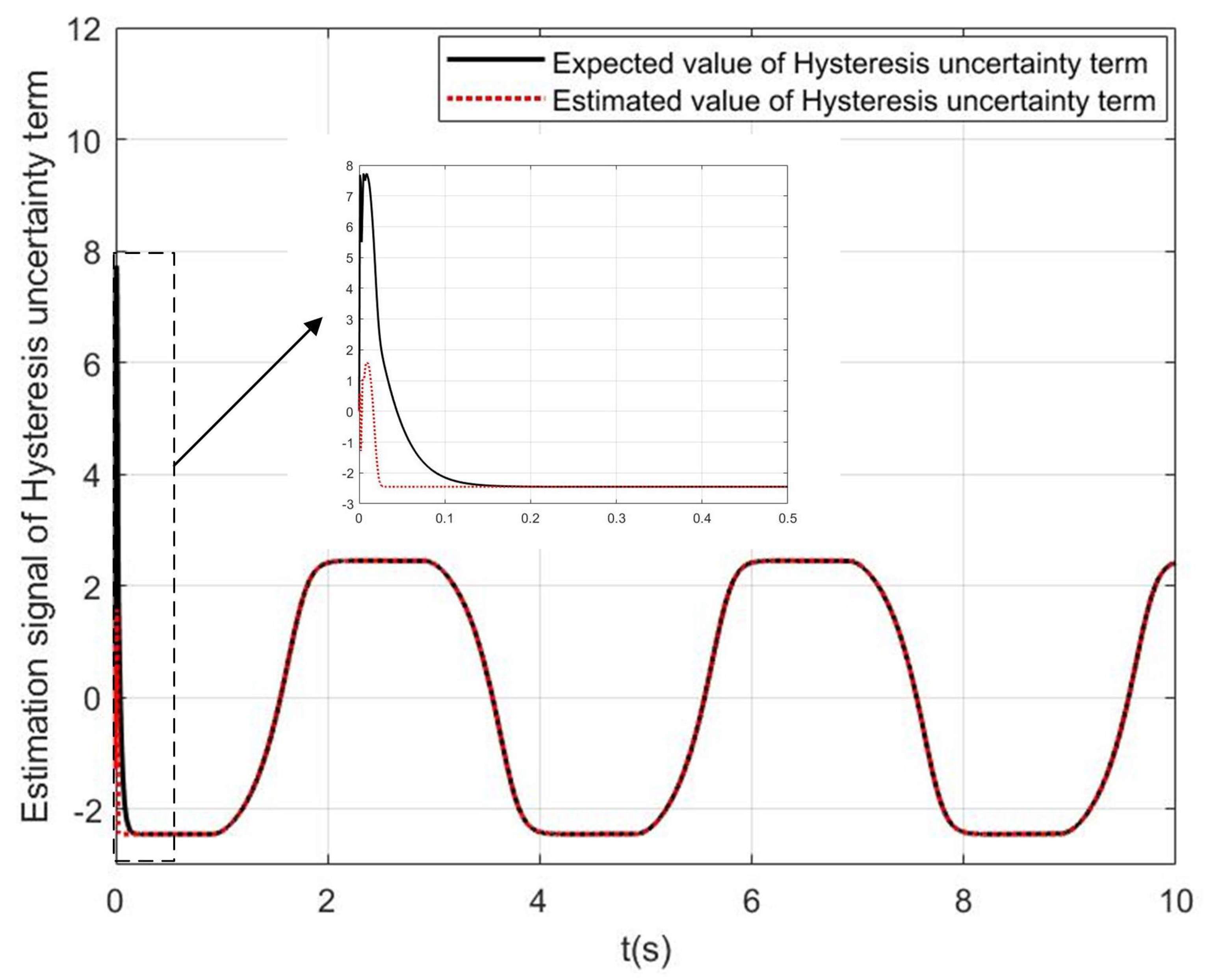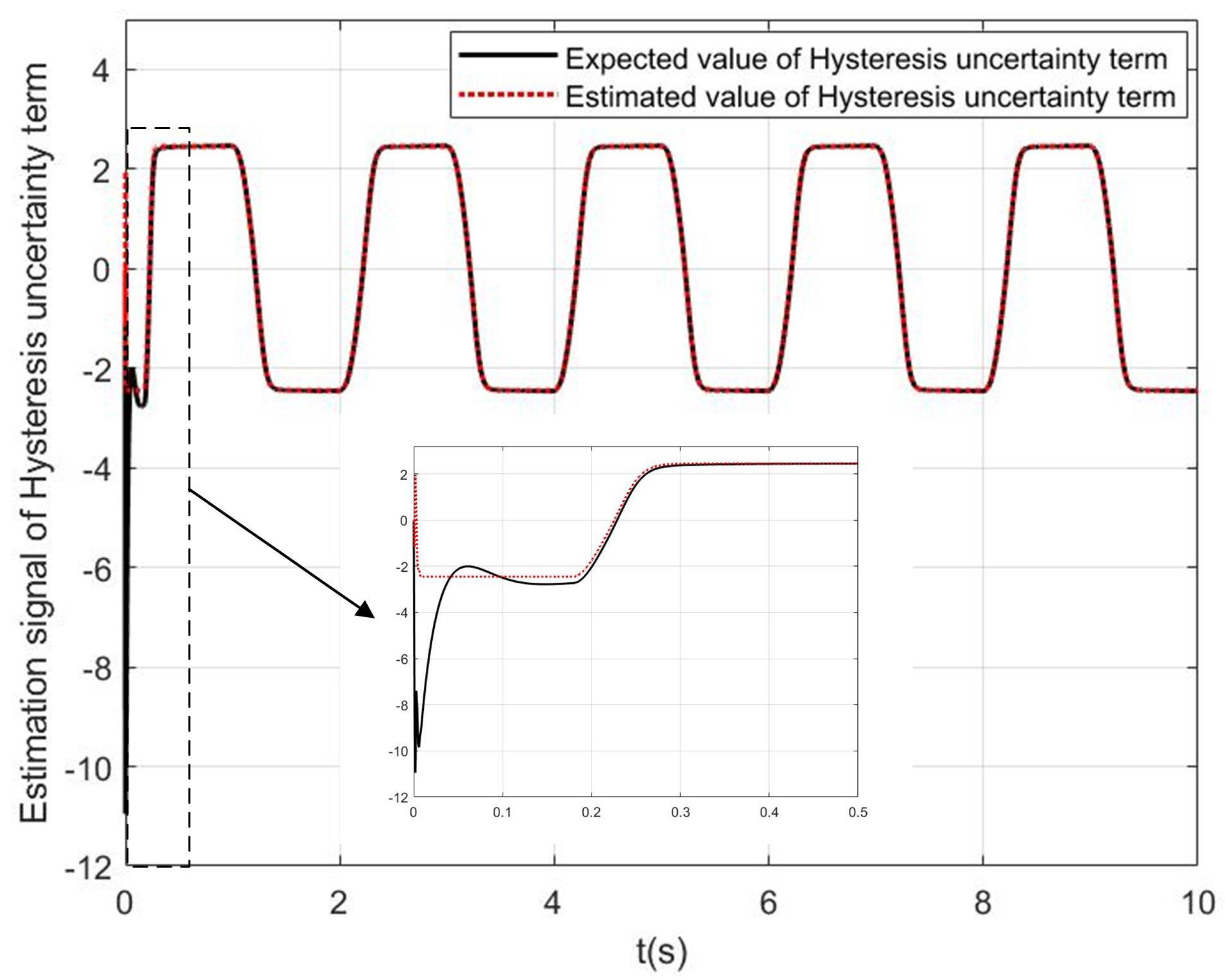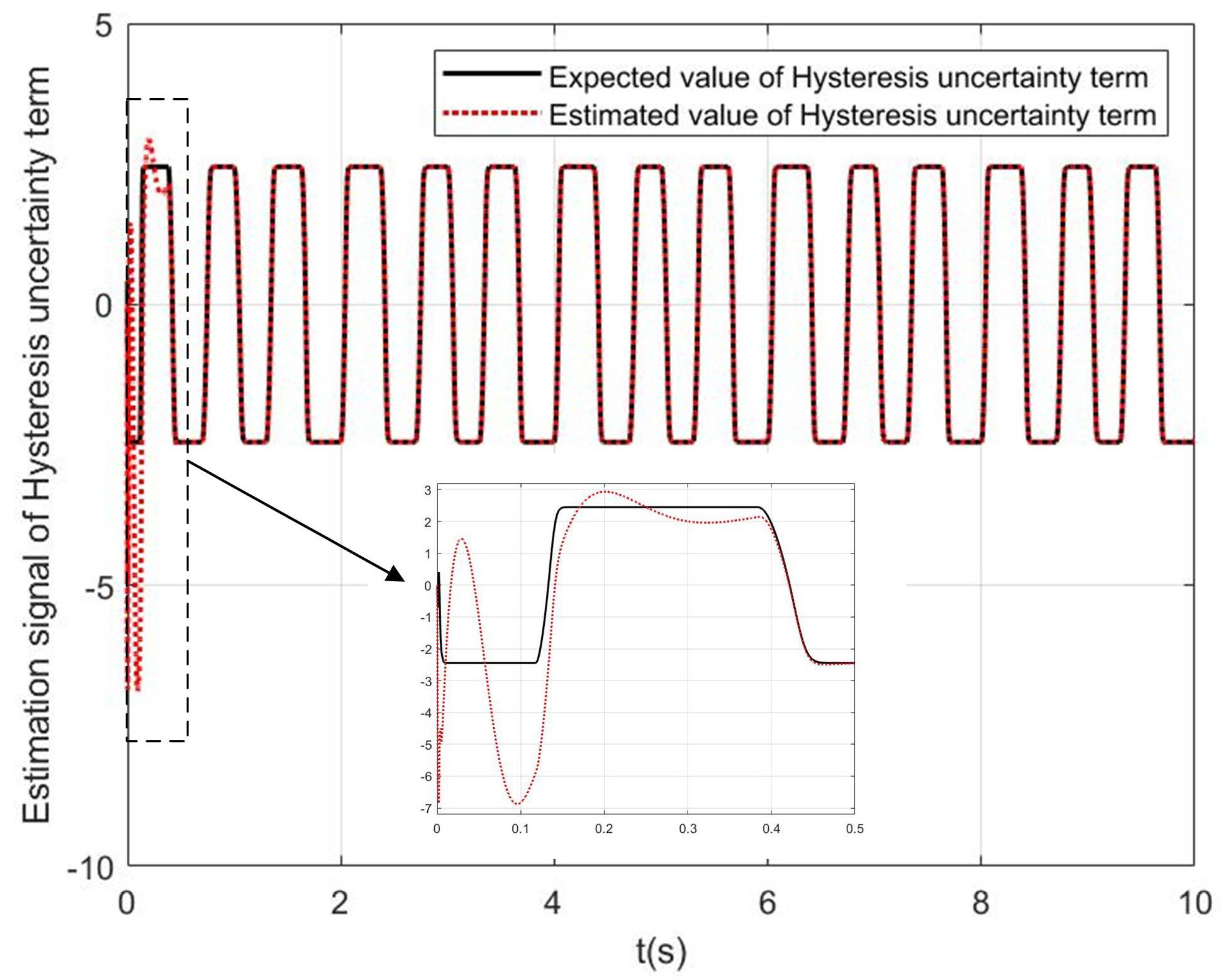Figure 4 shows the estimation of the hysteresis uncertainty term obtained using the time delay estimation technique. Since the model parameters of the controlled object are unknown, and the time delay estimator is derived from Equation (16), the estimator will also have a response process. It takes about 0.15 s to achieve a better estimate. Figure 5 shows the input–output relationship of the Bouc–Wen hysteresis under steady-state conditions when applying the algorithm proposed in this paper. It is apparent that the hysteresis phenomenon is clearly present and remains essentially stable and unchanged during the steady-state period.

To further validate the effectiveness of the adaptive backstepping time delay controller, this paper also conducted simulation tests on the following two relatively complex desired input trajectories: $x_{d2}=2sin\left(t\right)+1.2cos\left(\pi t\right)$, $x_{d3}=sin\left(t\right)+0.6cos\left(\pi t\right)+0.3cos\left(3\pi t\right)+0.4cos\left(2\pi t\right)$. The simulation results are shown in Figure 6, Figure 7, Figure 8, Figure 9, Figure 10 and Figure 11. From Figure 6 and Figure 9, it can be seen that the proposed control method achieves good tracking performance for complex input signals. This indicates that the control method possesses strong adaptability and maintains good control performance when faced with complex inputs. As seen from Figure 7 and Figure 10, the tracking error of the control method presented herein shows a significant advantage compared to the other two control methods. This demonstrates that the proposed method is effective in reducing tracking errors and improving control precision. Figure 8 and Figure 11 illustrate the comparison between the time delay estimation values and the actual values. It is clear that after a short transition period, the time delay estimator can accurately estimate the uncertain part of the hysteresis, which is crucial for compensating for the hysteresis phenomenon in control systems.

Overall, the summary of the simulation results is shown in

Table 1. Summary of simulation results (based on Figure 6, Figure 7, Figure 8, Figure 9, Figure 10 and Figure 11).

Serial Number	Control Method	Control Characteristics	Control Effect
1	Control method in [25]	Using classic time delay estimation technique, no need to construct an inverse hysteresis model	Medium tracking error
2	Control method in [32]	Treating the hysteresis term as a disturbance, no need to construct an inverse hysteresis model	Maximum tracking error
3	The proposed method	Using time delay estimation technology with error compensation; no need to construct an inverse hysteresis model	Minimum tracking error

. In Table 1, we list the characteristics and control effects of three comparison algorithms. Clearly, the tracking error of the controller proposed in this paper is the smallest, and it achieves the best control performance. The results above lead to the conclusion that the proposed control method is effective. This method can address the issue of compensation control for unknown hysteresis, enhancing the control performance and precision of the system.

5. Conclusions

For a class of second-order piezoelectric devices with unknown system parameters and hysteresis parameters, an adaptive control strategy based on time delay estimation technology is proposed in this paper. The control method primarily addresses three issues. Firstly, it achieves precise compensation control for hysteresis without the need to construct an inverse model of the hysteresis. Secondly, it tackles the control problem when both system parameters and hysteresis parameters are unknown, enhancing the adaptability of the controller. Thirdly, the control method is easily implementable in engineering due to the adoption of the mechanism of time delay estimation. Through simulations comparing with two representative control algorithms under three different input signals, the results demonstrate that the algorithm proposed in this paper has the smallest tracking error and achieves the best control performance. This further validates the effectiveness, superiority, and adaptability of the proposed control method.