DAGOR: Learning DAGs via Topological Sorts and QR Factorization

Abstract

Recently, the task of acquiring causal directed acyclic graphs (DAGs) from empirical data has been modeled as an iterative process within the framework of continuous optimization with a differentiable acyclicity characterization. However, learning DAGs from data is an NP-hard problem since the DAG space increases super-exponentially with the number of variables. In this work, we introduce the graph topological sorts in solving the continuous optimization problem, which is substantially smaller than the DAG space and beneficial in avoiding local optima. Moreover, the topological sorts space does not require consideration of acyclicity, which can significantly reduce the computational cost. To further deal with the inherent asymmetries of DAGs, we investigate the acyclicity characterization and propose a new DAGs learning optimization strategy based on QR factorization, named DAGOR. First, using the matrix congruent transformation, the adjacency matrix of the DAG is transformed into an upper triangular matrix with a topological sort. Next, using the QR factorization as a basis, we construct a least-square penalty function as constraints for optimization in the graph autoencoder framework. Numerical experiments are performed to further validate our theoretical results and demonstrate the competitive performance of our method.

1. Introduction

Causal directed acyclic graphs (DAGs) can effectively represent the inter-relationships between variables, which providing a powerful tool for uncertainty inference systems. In recent years, the research of DAGs has become a popular research area in artificial intelligence and machine learning [1,2,3]. Also, DAGs have been successfully applied in many fields such as social science [4,5], biomedicine [6,7] and economics [8,9]. Before utilizing DAGs for causal inference and uncertainty reasoning, it is important to learn the structure of DAGs from empirical data.

The domain of causal structure learning is broadly delineated into two principal categories, that constraint-based learning and score-based learning methodologies. Constraint-based learning methods generally apply the conditional independence (CI) tests or mutual information to identify dependence relationships between variables, and then build DAGs that satisfy these interactions. Typical constraint-based algorithms include Peter–Clark algorithm (PC) [10], Recursive Autonomy Identification (RAI) [11], Optimized Zero-First-Order Super-Structure (Opt01SS) [12], and so on. However, the constraint-based DAGs learning process is highly sensitive to test errors, and while one CI test is wrong it can directly influence the results of subsequent tests.

Therefore, compared to constraint-based learning methods, score-based learning methods are currently in more widespread usage. The score-based learning methods address the structural learning problems as model selection programs, which consist of three components: score function, search algorithm, and search space. The score function is used to evaluate the likelihood of the candidate structure fitting the empirical data. The search algorithm performs a searching strategy for the highest score structure in the candidate structures space and it adopts the heuristic search algorithm mostly. The search space is generally divided into three kinds: space composed of DAGs, space composed of DAG-equivalent class, and space composed of variable topological sorts. Traditional algorithms derived from the combinatorial optimization programs include K2 algorithm [13], Minimum Description Length and Evolutionary Programming (MDLEP) [14], PC-Particle Swarm Optimization (PC-PSO) [15], etc.

Furthermore, researchers gradually introduce deep learning methods into score-based DAGs learning, and transform the traditional combinatorial optimization problem into a continuous optimization process [16,17]. Search algorithms have also changed from heuristic search to deep generative model. This continuous optimization approach consists of two components: acyclicity characterization and deep generative model. On the one hand, the matrix acyclicity characterization is a precondition for the continuous optimization of DAGs, and mathematically, the adjacency matrix of DAG must be the nilpotent matrix. On the other hand, within the DAGs learning continuous optimization framework, more deep generative models are deployed for DAGs learning and show significant improvements, such as graph neural network, generative adversarial network, reinforcement learning, and generative flow network. But, in the face of larger data and higher accuracy requirements, there are still some challenges:

• Most DAGs continuous optimization are performed by searching in the DAG space. Once the number of DAG variables increases, the DAG space increases exponentially and the generative networks with large parameters cannot find a satisfactory DAG in finite time.
• Mathematically, the nilpotent matrix is always used to achieve the acyclicity characterization. In practice, each power operation indicates that it takes a step forward in the directed edge on the graph. However, as the graph size grows, the calculated power number increases, the complexity of the operation rises, and the efficiency of the model decreases.

For the first problem of super-exponential expansion of the DAG space faced by most of the methods, this paper adopts the topological sorts space solving algorithm. By transforming the adjacency matrix into an upper triangular matrix through a congruent transformation guided by the topological sorts, and then the parameters update during the training process only needs to be performed on half of the matrix elements. As the second problem, for continuous optimization based DAGs learning using nilpotent matrices to inscribe acyclic constraints, we decompose the adjacency matrices in training by using QR factorization and design the least-square penalty function instead of the nilpotent matrices, which makes the computation simpler and more efficient.

In this paper, we consider migrating the continuous optimization from the DAG space to the topological sorts space. The space of topological sorts is significantly smaller than the space of DAG or of the equivalence classes. Furthermore, we propose adopt congruent transformation and QR factorization to create an optimization strategy based on the topological sorts. In addition, we employ our method in a graph autoencoder network framework and generate satisfactory DAGs from the data. A summary of the main contributions of this paper is as follows:

• We propose continuous optimization DAGs learning in the topological sorts space. We express the topological sorts matrixically, and subsequently use a matrix congruent transformation to convert the initial adjacency matrix into an sort-based adjacency matrix, which enables the continuous optimization DAGs learning to be intervened with the topological sorts.
• Based on the topological sorts, we further improve the optimization strategy by using QR factorization. We perform a QR factorization of the sort-based adjacency matrix and utilize the upper triangular attribute of the decomposed matrix to construct the least-square penalty function as constraints for optimization.
• We employ our DAGs learning optimization strategy in a graph autoencoder network as the deep generative model framework. And we investigate a comparative analysis of our proposed method against a selection of contemporary algorithms on both synthetic datasets and real-world datasets. The results of our experiments demonstrate the effectiveness of our proposed method.

The subsequent sections of this paper are structured as follows. In Section 2, we introduce a thorough review of related works. Section 3 is dedicated to introducing the foundational preliminaries underpinning our study. And in Section 4, we propose a new DAGs learning method DAGOR. Section 5 reports our experiments and results. Finally, the conclusions of this study are summarized in Section 6.

2. Related Works

DAGs learning based on continuous optimization has become a popular research topic. There are two technological lines of research. One is the mathematical acyclicity characterization for DAGs constraint, and the other is the deep generative model for DAGs generation. The former focuses on matrix theoretical analysis for DAGs acyclicity, and the latter adopts deep learning approaches as DAGs generative models.

For acyclicity characterization studies, NO TEARS [16] is firstly solving the combinatorial graph search challenge into a continuous optimization paradigm through the utilization of trace exponential and nilpotent matrix methodologies. It is based on the gradient computation of the continuous score function. However, a notable limitation of this approach is the computationally intensive property of matrix exponential calculations, which require $O\left(d^3\right)$ operations. In response to this high computational complexity, NO BEARS [17] offers a different reformulation by leveraging the spectral radius of the adjacency matrix to bound DAGs acyclicity, effectively reducing computational complexity to $O\left(d^2\right)$. Furthermore, NO FEARS [18] introduces an innovative acyclicity characterization based on absolute values, which instead the Hadamard product in NO TEARS. This facilitates a practical solution for augmented Lagrangian optimization convergence. Building upon this foundation, GOLEM [19] proposes a likelihood-based score mechanism augmented with $l1$ regularization and soft acyclicity constraints. And NO TEARS+ [20] extends the acyclicity characterization to accommodate nonparametric general models. LEAST [21] presents a novel acyclicity constraint paradigm, enhancing upon NO BEARS by leveraging least-square objectives and $l1$ regularization, achieving computational efficiency closer to $O\left(d\right)$. DAGMA [22] eliminates NO TEARS power series and introduces a log-determinant acyclicity characterization. However, these above methods are calculating in the DAG space and with strict limitations for acyclic characterization, which means they are always stuck in a local optimum. But our proposed method, DAGOR, which operates in a topological sorts space with a global modification to the hypothesis, avoids local optima and does not require consideration of acyclicity, reducing computational costs significantly.

As for the DAGs deep generative models, CGNN [23] firstly represents an integration of continuous optimization for DAG learning with neural networks. Subsequent innovations include Graphite [24], which employs a generative neural network framework to reconstruct DAGs parameterized by weighted adjacency matrices. But its initial output is an undirected graph. SAM [25] introduces adversarial training strategies to optimize end-to-end DAG learning, enhancing model robustness. DAG-GNN [26] integrates neural network functions and black-box variational inference into DAGs learning methods, leveraging evidence lower bound (ELBO) [27,28] as the score criterion. Expanding upon this paradigm, GAE [29] extends DAG-GNN formalisms to a graph autoencoder framework, facilitating the incorporation of non-linear structural interactions and vector-valued variables. RL-BIC [30] adopts a reinforcement learning approach to DAGs learning and causal discovery, where the reward function consists of a BIC scoring function and an acyclic constraint function with a penalty term. In addition, DAG-GAN [31] devises an adversarial framework for DAGs structure detection. DAG-GFlowNet [32] proposes to use the generative flow networks for approximating the posterior distribution over the structure of DAGs. GraN-DAG [33] learns the conditional independent relationship of the neural network model between variables and transforms the problem into the maximum likelihood optimization problem. It utilizes a multilayer perceptron and a continuous acyclic constraint function as a loss function to constrain its acyclicity.

In particular, we investigate the characteristics of the above methods in

Table 1. Methods description: Type I represents researching mathematical acyclicity characterization for DAGs constraint; Type II indicates utilizing deep generative model for DAGs generation.

Method	Year	Type	Data	Acyclicity	Output
NOTEARS	2018	I	Low	Yes	DAG
CGNN	2018	II	Low	Yes	DAG
Graphite	2019	II	Low/Medium	No	UG
SAM	2019	II	Low/Medium	Yes	DAG
DAG-GNN	2019	II	Low	Yes	DAG
GAE	2019	II	Low	Yes	DAG
NOBEARS	2019	I	Low/Medium/High	Yes	DAG
NOFEARS	2020	I	Low	Yes	DAG
GOLEM	2020	I	Low	Yes	DAG
RL-BIC	2020	II	Low	Yes	DAG
GraN-DAG	2020	II	Low	Yes	DAG
NOTEARS+	2020	I	Low	Yes	DAG
LEAST	2020	I	Low/Medium/High	Yes	DAG
DAG-GAN	2021	II	Low	Yes	DAG
DAG-GFlowNet	2022	II	Low	Yes	DAG
DAGMA	2022	I	Low/Medium/High	Yes	DAG

, as they are the latest advancements in the domain of DAGs learning. We also compare them to the above deep generative models, including NOTEARS, GraN-DAG, DAG-GNN, and RL-BIC. DAGOR has an efficient performance because after the topological sorts based upper triangularization, the adjacency matrix in training only needs to be updated with half of the parameter values.

According to the above analysis, we conclude mostly DAGs learning research concentrates on acyclicity characterization and deep generative models. However, precisely learning DAGs from data is still a challenging problem.

3. Preliminaries

3.1. Directed Acyclic Graphs

A graph is fundamentally composed of vertices and edges, and the edges establish connections between pairs of vertices. The vertices can also represent a myriad of entities, which are linked together in pairs through the intermediary of edges. In the directed graphs, each edge possesses a distinct orientation, which represents a directional flow from one vertex to another. Formally, a path within a directed graph comprises a sequence of edges, where each subsequent edge commences from the vertex of its predecessor. It is worth noting that directed acyclic graphs are characterized by the absence of cycles or closed loops, distinguishing them as structures devoid of cyclical dependencies.

As for directed graphs, the notion of reachability between vertices assumes significance. A vertex v is reachable from another vertex u if there exists a path originating at u and concluding at v. It follows that if a vertex can traverse a nontrivial path to reach itself, then this path necessarily constitutes a cycle. Consequently, an alternative characterization of DAGs emerges: the graphs wherein no vertex can traverse a nontrivial path to reach itself [34].

In addition, the DAG is a significant tool for portraying causal effects and causality. The directed edges represent vertices from cause to effect, which reflects causal effects cannot be bidirectional.

3.2. Topological Sorts

A DAG can be topologically sorted by arranging its vertices in a sequence, which ensures a logical flow of information and makes it easier to understand the relationships between the vertices. In the graph theory, a discernible characteristic of a topological sort is its inherent prohibition of cycles, as the directional orientation of edges makes a unidirectional flow that precludes the existence of cycles. Conversely, every DAG has at least one topological sort. Hence, the presence of a topological sort emerges as an equivalent criterion for DAGs. It is important to acknowledge that the uniqueness of this sort is not universal; a DAG owns a singular topological sort exclusively when it has a directed path encompassing all vertices. In such instances, the sequential arrangement of vertices within the topological sort reflects their sort along the aforementioned path, thereby illuminating a distinct correlation between the topology of the graph and the linear arrangement of its vertices [35].

Moreover, the family of DAGs topological sorts coincide with the family of linear extensions derived from its reachability relation [36], which representing the intrinsic relationship between the structural properties of the graphs and the resultant arrangements yielded by their topological sorts.

3.3. Determine Acyclicity Based on DAGs Adjacency Matrix

The DAG consists of its vertex set $V\left(G\right)$ and edge set $E\left(G\right)$, where the elements of $E\left(G\right)$ are all binary subsets of $V\left(G\right)$. Let ${\left(A\right)}_{ij}$ represents the $(i,j)$-position element of matrix A. For a graph G with n vertices, its adjacency matrix $A_G$ is an $n\times n$ matrix whose elements are defined as

$${\left(A_G\right)}_{ij}=\left\{\begin{array}{cc}1,\hfill & ij\in E\left(G\right),\hfill \\ 0,\hfill & ij\notin E\left(G\right).\hfill \end{array}\right.$$

(1)

Based on the attributes of DAGs, the adjacency matrix $A_G$ has the following three properties:

• The diagonal coefficients of matrix $A_G$ are all zeros;

  $${\left(A_G\right)}_{ij}=0,s.t.i=j$$
• Matrix $A_G$ is an asymmetric matrix;

  $${A_G}^{\mathsf{T}}\ne A_G$$
• Matrix $A_G$ is a nilpotent matrix.

  $${A_G}^n={\left[0\right]}_{n\times n}$$

Specifically, each exponentiation of the adjacency matrix $A_G$ symbolizes a singular step in the vertex transition process within the graph. Consequently, the resultant nilpotent matrix signifies a state wherein all elements of ${A_G}^n$ are rendered as zeros after taking n consecutive power operations. This denotes that the vertices within the graph fail to cyclically return to their initial states following n steps of transition, thereby unequivocally indicating the absence of any closed-loop structures within the graph.

4. Proposed Method

In this section, we introduce our method DAGOR. In this method, we firstly conduct adjacency matrix congruent transformation based on the topological sort vector. Secondly, we perform the QR factorization of the transformed adjacency matrix and propose a least-square penalty function with the upper triangular matrix as constraints for the DAGs learning process. Finally, we employ the DAGOR algorithm with a graph autoencoder framework.

Learning DAGs using topological sorts and QR factorization is carried out because we fin that during the training process of learning DAGs based on deep generative models, the adjacency matrix is normally the one that needs to be updated iteratively for all matrix elements. This is very inefficient for complex datasets with more vertices. Therefore, we consider designing a topological sorts based contract matrix transformation to upper triangularize the adjacency matrix so that only half of the matrix parameters need to be updated for each training. Further, we find that upper triangular matrices also exist in QR factorization, which is consistent with the adjacency matrix in training. Therefore, we introduce QR factorization into the training objective to construct least-square penalty function as constraints for optimization.

4.1. Adjacency Matrix Congruent Transformation with Topological Sorts

In the context of graph theory, a topological sort for a directed graph G is a partial ordering denoted as ≺ on its vertex set $V=\left[p\right]$. This sort corresponds to the condition that for any vertices $X_i$ and $X_j$ in V, the presence of a directed edge from $X_i$ to $X_j$ ($X_i\to X_j$) implies $i\prec j$. The symbol $X_i\to X_j$ denotes the existence of an edge between vertices i and j.

A topological sort, denoted by ≺, defines a permutation $\pi$ on the vertex set V of graph G. This permutation assigns $\pi \left(i\right)$ to the vertex at the i-th position in the ordering specified by ≺. Importantly, a topological sort yields a unique arrangement of vertices in G.

$$\begin{array}{cc}\hfill \pi & =\left[i\right],i\in \{1,2,\cdots ,n\}\hfill \\ \hfill s.t.& i\prec j;X_i\to X_j\mathbf{in}G.\hfill \end{array}$$

(2)

Moreover, a directed graph is acyclic if and only if it possesses a topological sort. It is important that the topological sort need not be unique for a given acyclic directed graph. Thus, the existence of a topological sort serves as a decisive criterion for identifying the acyclic characterization of a directed graph, emphasizing its key role in graph theory.

In mathematics, the congruence of two square matrices, denoted as A and B, defined over a field, is established when there exists an invertible matrix P over the same field. This congruence relationship is expressed as

$$P^{\mathsf{T}}AP=B,$$

(3)

where $P^{\mathsf{T}}$ denotes the transpose of the matrix P.

Therefore, we conduct the DAGs adjacency matrix congruent transformation with topological sorts. For each permutation $\pi$ on the set $\left[p\right]:=\{1,2,\cdots ,p\}$, we correspondingly establish a permutation matrix $P_{\pi }$, with its i-th row being denoted as $e_{\pi }^{\mathsf{T}}\left(i\right)$. Given a vector $v={(v_{\pi \left(1\right)},\cdots ,v_{\pi \left(p\right)})}^{\mathsf{T}}$, we observe that the operation $P_{\pi }v$ results as:

$$P_{\pi }v=v_{\pi }={(v_{\pi \left(1\right)},\dots ,v_{\pi \left(p\right)})}^{\mathsf{T}},$$

(4)

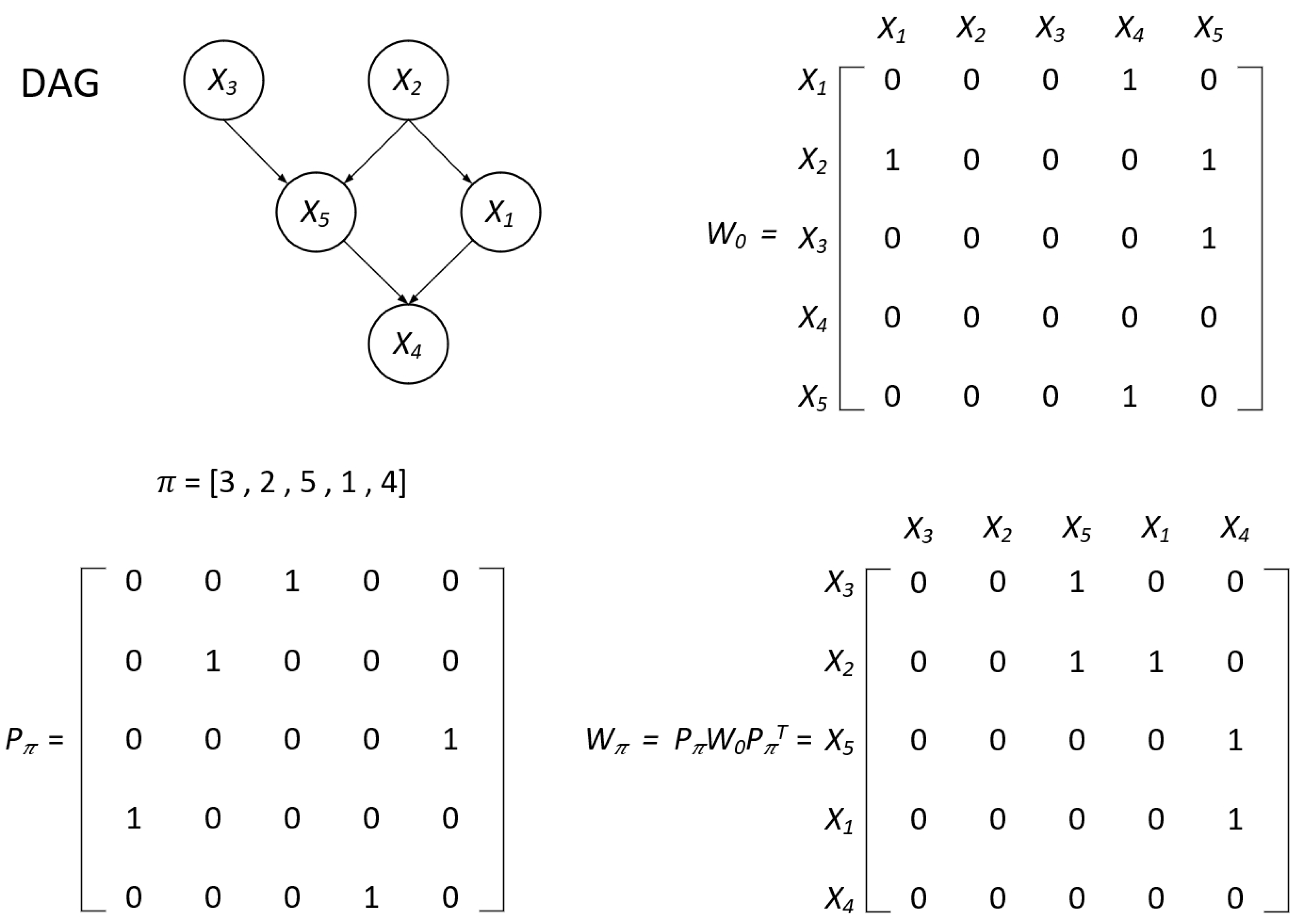
signifying that $P_{\pi }$ systematically rearranges the entries of vector v in accordance with the permutation $\pi$ and $P_{\pi }^T{P}_{\pi }=I$. Thus, we perform a congruent transformation of the original adjacency matrix $W_0$ of $A_G$, let

$$W_{\pi }:=P_{\pi }{W}_0{P}_{\pi }^{\mathsf{T}}.$$

(5)

Subsequently, the matrix $W_{\pi }$ takes on the form of a strictly upper triangular matrix if and only if $\pi$ represents the topological sort of the directed acyclic graph G, denoted by $i\prec j$ in $\pi$ for $j\in {\Pi }_i^G$. A visual representation is provided in Figure 1 for enhanced clarity. Consequently, the acyclicity condition on $W_0$ translates to the requirement that $W_{\pi }$ assumes a strictly upper triangular form for a specific permutation sort $\pi$. And we can further utilize $W_{\pi }$ for next DAGs optimization.

4.2. QR Factorization for the Transformed Adjacency Matrix

A recognized matrix factorization refers to a linear transformation that analyses an acknowledged matrix into a product of two or three matrices, typically of standard types. One prominent instance of such factorization is the QR factorization. This factorization entails breaking down the matrix into the product of an orthogonal matrix and a triangular matrix. Specifically, the QR factorization of a real square matrix A is characterized by the expression

$$A=QR.$$

(6)

In this factorization, Q represents an orthogonal matrix with columns comprising orthogonal unit vectors, denoted by $Q^{\mathsf{T}}=Q^{-1}$, and R is an upper triangular matrix. In the case of a nonsingular matrix A, this factorization is uniquely determined. Conversely, for a complex square matrix A, an analogous factorization $A=QR$ exists, but with Q being a unitary matrix, characterized by the property that its conjugate transpose, denoted as $Q^{†}$, is equal to its inverse, i.e., $Q^{†}=Q^{-1}$.

Various methodologies exist for computing the QR factorization, including the Gram–Schmidt process [37], Householder transformations [38], and Givens rotations [39]. In our DAGOR framework, we employ the Gram–Schmidt process. The procedure involves considering the vectors to be processed as columns of the matrix A. That is,

$$A=\left[\begin{array}{cccc}{\mathbf{a}}_1& \left|{\mathbf{a}}_2\right|& \cdots & |{\mathbf{a}}_n\end{array}\right].$$

(7)

Then,

$$\begin{array}{cc}\hfill {\mathbf{u}}_1& ={\mathbf{a}}_1,{\mathbf{e}}_1=\frac{{\mathbf{u}}_1}{\left|\right|{\mathbf{u}}_1\left|\right|},\hfill \\ \hfill {\mathbf{u}}_2& ={\mathbf{a}}_2-({\mathbf{a}}_2·{\mathbf{e}}_1){\mathbf{e}}_1,{\mathbf{e}}_2=\frac{{\mathbf{u}}_2}{\left|\right|{\mathbf{u}}_2\left|\right|},\hfill \\ \hfill {\mathbf{u}}_{k+1}& ={\mathbf{a}}_{k+1}-({\mathbf{a}}_{k+1}·{\mathbf{e}}_1){\mathbf{e}}_1-\cdots -({\mathbf{a}}_{k+1}·{\mathbf{e}}_k){\mathbf{e}}_k,{\mathbf{e}}_{k+1}=\frac{{\mathbf{u}}_{k+1}}{\left|\right|{\mathbf{u}}_{k+1}\left|\right|}.\hfill \end{array}$$

(8)

Note that $\left|\right|·\left|\right|$ is the $l2$ norm. The resulting QR factorization is

$$\left.A=\left[\begin{array}{cccc}\hfill {\mathbf{e}}_1& \hfill \left|{\mathbf{e}}_2\right|& \hfill \cdots & \hfill |{\mathbf{e}}_n\end{array}\right.\right]\left[\begin{array}{cccc}\hfill {\mathbf{a}}_1·{\mathbf{e}}_1& \hfill {\mathbf{a}}_2·{\mathbf{e}}_1& \hfill \cdots & \hfill {\mathbf{a}}_n·{\mathbf{e}}_1\\ \hfill 0& \hfill {\mathbf{a}}_2·{\mathbf{e}}_2& \hfill \cdots & \hfill {\mathbf{a}}_n·{\mathbf{e}}_2\\ \hfill ⋮& \hfill ⋮& \hfill \ddots & \hfill ⋮\\ \hfill 0& \hfill 0& \hfill \cdots & \hfill {\mathbf{a}}_n·{\mathbf{e}}_n\end{array}\right]=QR.$$

(9)

Note that once we find $e_1,\cdots ,e_n$, it is not hard to write the QR factorization.

In the training phase of the depth generation model, the resultant adjacency matrix is denoted as W. Following the acquisition of the topological sort ${\pi }^{*}$ through the topological sorts learning methods [40,41], a matrix $\pi$ is introduced to represent $P_{{\pi }^{*}}$, and a contracted matrix operation is applied:

$$W_{{\pi }^{*}}=P_{{\pi }^{*}}W{P}_{{\pi }^{*}}^{\mathsf{T}}.$$

(10)

The primary objective of the training process is to ensure that W accurately reflects the adjacency matrix of DAGs, while $W_{{\pi }^{*}}$ is specifically represented as the upper triangular matrix. Based on the QR factorization, the adjacency matrix

$$W=QR,$$

(11)

where Q is the orthogonal matrix and R is the upper triangle matrix. By the definition of an orthogonal matrix Q, an orthogonal matrix must be an invertible matrix:

$$Q{Q}^{\mathsf{T}}=Q{Q}^{-1}=I.$$

(12)

Then we can also express the upper triangle matrix R as follows:

$$R=Q^{-1}W.$$

(13)

Thus, when $W\to W_{{\pi }^{*}}$, Q converges to the unit matrix, i.e., $Q\to I$. Therefore, we propose to set the training optimization satisfying

$$h\left(W\right)=\frac{1}{2n}||P_{\pi }W{P}_{\pi }^{\mathsf{T}}-Q^{-1}\left(P_{\pi }W{P}_{\pi }^{\mathsf{T}}\right)|{|}^2;h\left(W\right)\to 0.$$

(14)

4.3. Algorithm with the Graph Autoencoder Framework

We use a deep generative model based on graph autoencoder (GAE) as a generative model framework. The GNNs framework for DAGs generation is designed as a variational autoencoder (VAE),

$$\begin{array}{c}Z=f_2((I-W^{\mathsf{T}})f_1\left(X\right))\\ \widehat{X}=f_4({(I-W^{\mathsf{T}})}^{-1}{f}_3\left(Z\right)).\end{array}$$

(15)

Here, $f_1$ can represent any parameterized graph neural network such as Graph Convolutional Network (GCN), Multilayer Perceptron (MLP), etc. Because a simple MLP is sufficiently effective for the generation of fitting data distributions, more complex models are not necessary. We define the MLP as $f_1$ and the identity mapping as $f_2$. Let $f_4$ be the MLP and $f_3$ be the constant mapping of the generative model.

$$\begin{array}{cc}\hfill Z& =(I-W^{\mathsf{T}}){\mathrm{MLP}}^1\left(X,{\omega }_1\right)\hfill \\ \hfill \widehat{X}& ={\mathrm{MLP}}^2({(I-W^{\mathsf{T}})}^{-1}Z,{\omega }_2),\hfill \end{array}$$

(16)

where ${\omega }_1$ and ${\omega }_2$ are the parameters of the neural network. By aggregating the samples $X=(X_1,\dots ,X_n)$ to assess the distributional specification of Z, the Kullback–Leibler (KL) divergence serves as a metric for quantifying the disparity between the variational distribution $q\left(Z\right|X)$ and the true posterior distribution $p\left(Z\right)$. Consequently, this methodology enables the inference of the generative model for the DAGs by maximizing the lower bound of evidence, known as the Evidence Lower Bound (ELBO).

$$L_{\mathrm{ELBO}}=-D_{\mathrm{KL}}\left(q\left(Z\right|X)\right|\left|p\left(Z\right)\right)+{\mathrm{E}}_{q\left(Z\right|X)}\log p\left(Z\right).$$

(17)

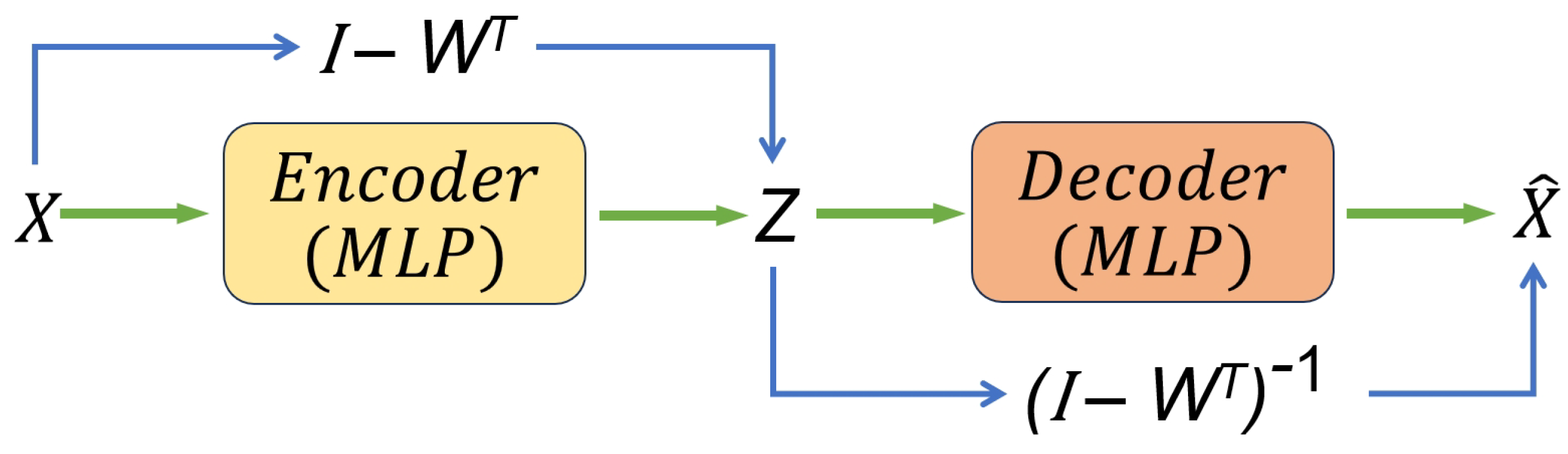
The encoder module operates by transforming a given sample denoted as ${\widehat{X}}^k$ into a representation characterized by the probability density function $p({\widehat{X}}^k|Z)$. Subsequently, the decoder module endeavors to reverse this process by reconstructing the original data $X^K$ from the latent variable Z, with the probability density $q\left(Z\right|X^K)$. The objective is to ensure that the generated sample $\widehat{X}$ is virtually indistinguishable from the true data X.

In this goal, the iterative training of the generative model is performed, facilitating the generation of synthetic data $\widehat{X}$ that closely approximates the true distribution X. This iterative generative training process ultimately culminates in the derivation of a highly satisfactory DAG adjacency matrix denoted as W. The matrix W encapsulates the relationships and dependencies within the data, thereby providing a robust and accurate representation of the underlying data structure. The model architecture is shown as Figure 2.

Hence, the final optimization problem is to minimize the reconstruction error of the GAE (with $l1$ penalty) within the least-square penalty function based on QR factorization as constraints:

$$\begin{array}{cc}\hfill \underset{W,\theta }{min}& F(W,\theta )=-L_{\mathrm{ELBO}}+\lambda {\parallel W\parallel }_1\hfill \\ \hfill \mathrm{s}.\mathrm{t}.& h\left(W\right)=\frac{1}{2n}||P_{\pi }W{P}_{\pi }^{\mathsf{T}}-Q^{-1}\left(P_{\pi }W{P}_{\pi }^{\mathsf{T}}\right)|{|}^2=0.\hfill \end{array}$$

(18)

Further derive its Lagrange function as

$$L(W,\theta ,\alpha )=-L_{\mathrm{ELBO}}+{\lambda \parallel W\parallel }_1+\alpha (\frac{1}{2n}\left|\right|P_{\pi }W{P}_{\pi }^{\mathsf{T}}-Q^{-1}\left(P_{\pi }W{P}_{\pi }^{\mathsf{T}}\right)\left|{|}^2\right),$$

(19)

$\alpha$ is the Lagrange multiplier, so its dual function is

$$g\left(\alpha \right)=\underset{W,\theta }{inf}L(W,\theta ,\alpha ).$$

(20)

Therefore, by iteratively descending the gradient to further solve its dual function, the solution of the original problem can be obtained. And as the GAE’s empirical default settings, we keep the coefficient $\lambda$ to 1.0.

5. Experiments

To assess the effectiveness of our proposed methodology, we systematically evaluate its performance through comparative analyses with established DAGs learning approaches on meticulously constructed simulated synthetic datasets and on benchmark datasets obtained from the Bayesian Network (BN) repository (https://www.bnlearn.com/bnrepository/, accessed on 6 February 2024).

In this section, the compared methods include NOTEARS [16], GraN-DAG [33], DAG-GNN [26] and RL-BIC [30]. NOTEARS firstly conduct continuous optimization on acyclic constraint, and GraN-DAG algorithm is an improvement of NOTEARS based on the neural network model. Similar to GraN-DAG, DAG-GNN is an enhancement of the NOTEARS algorithm based on variational inference and graph neural networks. And the RL-BIC algorithm is the first model to introduce reinforcement learning into DAG learning domain.

In Section 5.2, we conduct experiments on the simulated synthetic datasets, which include linear Gaussian SEM datasets from an Erdős–Rényi (ER) graph and non-linear multilayer perceptron (MLP) SEM datasets from a scale-free (SF) graph. Evaluation metrics include True Positive Rate (TPR), precision, F1 score, and Structural Hamming Distance (SHD), which is used to determine the gap between learned and true structure.

In Section 5.3, we analyse the capability of our model on the benchmark datasets, including SACHS [42], INSURANCE [43], ALARM [44], and HAILFINDER [45]. We specially compared all methods with groundtruth. We further utilize the Bayesian Dirichlet equivalent uniform (BDeu), Bayesian Information Criterion (BIC) scores as evaluation criteria to judge the ability of the DAGOR model to search for optimally DAGs structure.

All algorithms are implemented and executed in Pytorch in a PC with 12th Gen Intel(R) Core(TM) i9-12900H @2.50 GHz, 64 bits, and 16.0 GB of memory. The code can be found at https://github.com/haozuo17/DAGOR, accessed on 6 February 2024.

5.1. Experiment Details

5.1.1. Datasets

Erdős–Rényi (ER) graph: Let $0\le p\le 1$ be the probability value and let n be a positive integer. The undirected graph on n vertices, with an edge $(v,w)$ connecting each pair of vertices $v,w$ with probability p, is defined as the graph $G(n,p)$.

Scale-free (SF) graph: A scale-free network is a connected graph wherein the number of links, denoted as k, emanating from a specific vertex follows a power-law distribution, represented as $P\left(k\right)\sim k^{-\gamma }$. The construction of a scale-free network involves the iterative addition of vertices to an existing network. In the procedure, connections are added to vertices that already have preferred attachment, making sure that the likelihood of connecting to a certain vertex i is exactly proportional to the quantity of links that vertex already has, $k_i$, i.e.,

$$P\left(\mathrm{linking}\mathrm{to}\mathrm{vertex}i\right)\sim \frac{k_i}{{\sum }_j{k}_j}.$$

5.1.2. Metrics

True Positive Rate (TPR) denotes the proportion of samples that were actually positive classes that were correctly predicted to be positive classes.

Precision indicates the ratio of the total number of positive pairs to the total number of positive pairs predicted.

F1 score can be seen as a kind of reconciled average of model precision and TPR.

Structure Hamming distance (SHD) is a common metric for measuring structure learning and it counts the total number of additions, deletions, and reversals of edges that are required to transform the estimated graph into the genuine graph.

5.1.3. Score Functions

Bayesian Information Criterion (BIC) score: The likelihood estimate of the probability distribution $P\left(\mathcal{D}\right|\mathcal{G})$ given the observed data and the BIC score function added penalties regarding the complexity of the model to the likelihood estimates:

$$\begin{array}{cc}\hfill S_{BIC}& =\sum _{i=1}^n\left(\sum _{j=1}^{r_{{\Omega }_i}}\sum _{k=1}^{r_i}{m}_{ijk}\log {\theta }_{ijk}-\frac{r_{{\Omega }_i}(r_i-1)}{2}\log m\right).\hfill \end{array}$$

where $m_{ijk}$ denotes the number of times the random variable $X_i$ in the observed data $\mathcal{D}$ takes the k-th value and its parent set of vertices takes the j-th combination of values.

Bayesian Dirichlet equivalence uniform (BDeu) score: When the prior distribution of the parameters $P\left({\theta }_{\mathcal{G}}\right|\mathcal{G})$ is assumed to satisfy the product Dirichlet distribution, the following can be derived:

$$\begin{array}{cc}\hfill S_{BDeu}& =\sum _{i=1}^n\left(\sum _{j=1}^{r_{{\Omega }_i}}\sum _{k=1}^{r_i}\log \frac{\Gamma \left(\sum {\alpha }_{ij*}\right)}{\Gamma \left(\sum ({\alpha }_{ij*}+n_{ij*})\right)}+\sum _{k=1}^{r_i}\log \frac{\Gamma \left({\alpha }_{ijk}+n_{ijk}\right)}{\Gamma \left({\alpha }_{ijk}\right)}\right).\hfill \end{array}$$

where $\Gamma$ denotes the gamma function, n denotes the number of random variables, $r_{{\Omega }_i}$ denotes the number of possible values of the set of parents of the i-th random variable $X_i$, $r_i$ denotes the number of possible values of the random variable $V_i$, $n_{ijk}$ denotes the number of samples when the random variable $V_i$ is taken to be k, and the set of parents of the random variable $V_i$ is taken to be j, and ${\alpha }_{ijk}$ is the Dirichlet parameter.

5.2. Synthetic Datasets Experiments

5.2.1. Linear Datasets Experiments

For linear structural equation models, it can be expressed as

$$X_i=w_i^{\top }{X}_i+Z_i,$$

(21)

where $W=[w_1\mid \cdots \mid w_d]\in {\mathbb{R}}^{d\times d}$ is the weighted adjacency matrix, and $Z_i\in \mathbf{R}$ represents the Gaussian noise.

Then, considering the ground-truth DAG derived from an ER2 graph, which encompasses d vertices and $2d$ edges, we assigned independent edge weights from a uniform distribution of $\left(\right[-2,-0.5]\cup [0.5,2\left]\right)$ to create a weight matrix W. Gaussian noise, $Z_i\sim \mathcal{N}(0,1),\forall i\in \left[d\right]$. Under these conditions, we generated random linear datasets $X\in {\mathbb{R}}^{n\times d}$. Each simulation involved generating $n=1000$ samples and conducting experiments on four graph sizes $d\in \{10,20,40,60\}$.

As illustrated in Figure 3, we find that DAGOR performs at a moderate level on the synthetic linear Gaussian SEM ER2 dataset. In the TPR figure, at 10 vertices, DAGOR has a high value, but as the number of vertices increases to 20, 40, 60, the performance of DAGOR begins to fluctuate and generally decreases. Moreover, the precision of DAGOR is not high, which suggests that there are some edges that are misdirected. For the F1 score, DAGOR has better performances than the reinforcement learning based algorithm RL-BIC and the neural network based algorithm GraN-DAG.

The reason why our DAGOR gets negative performance on ER2 graphs is because the performance of the DAGOR algorithm partially depends on the reliability of the topological sorts. If the topological order is not exact, it will have an impact on the DAGOR search algorithm. However, in the ER2 graphs structure, there are a lot of juxtaposed vertices, which disturbing to the topological sorts and resulting a fuzzy search space. This always reduces the ability of DAGOR to discover DAGs from the vertex topological sorts.

5.2.2. Non-Linear Datasets Experiments

For non-linear structural equation models, we simulate as

$$X_i=f_i\left(X_{\mathrm{pa}\left(i\right)}\right)+Z_i,$$

(22)

where $f_i$ represents a multilayer perceptron (MLP) that has been randomly initialized, one hidden layer, size 100, and sigmoid activation. $X_{\mathrm{pa}\left(i\right)}$ represents the set of parent vertices and $Z_i\sim \mathcal{N}(0,1)$ is a standard Gaussian noise.

In this part, we take scale-free (SF) graph as ground-truth DAG derivation. Similar to linear experiments, we generate datasets $X\in {\mathbb{R}}^{n\times d}$ from SF2, with $n=1000$ i.i.d. samples and graph size $d\in \{10,20,40,60\}$.

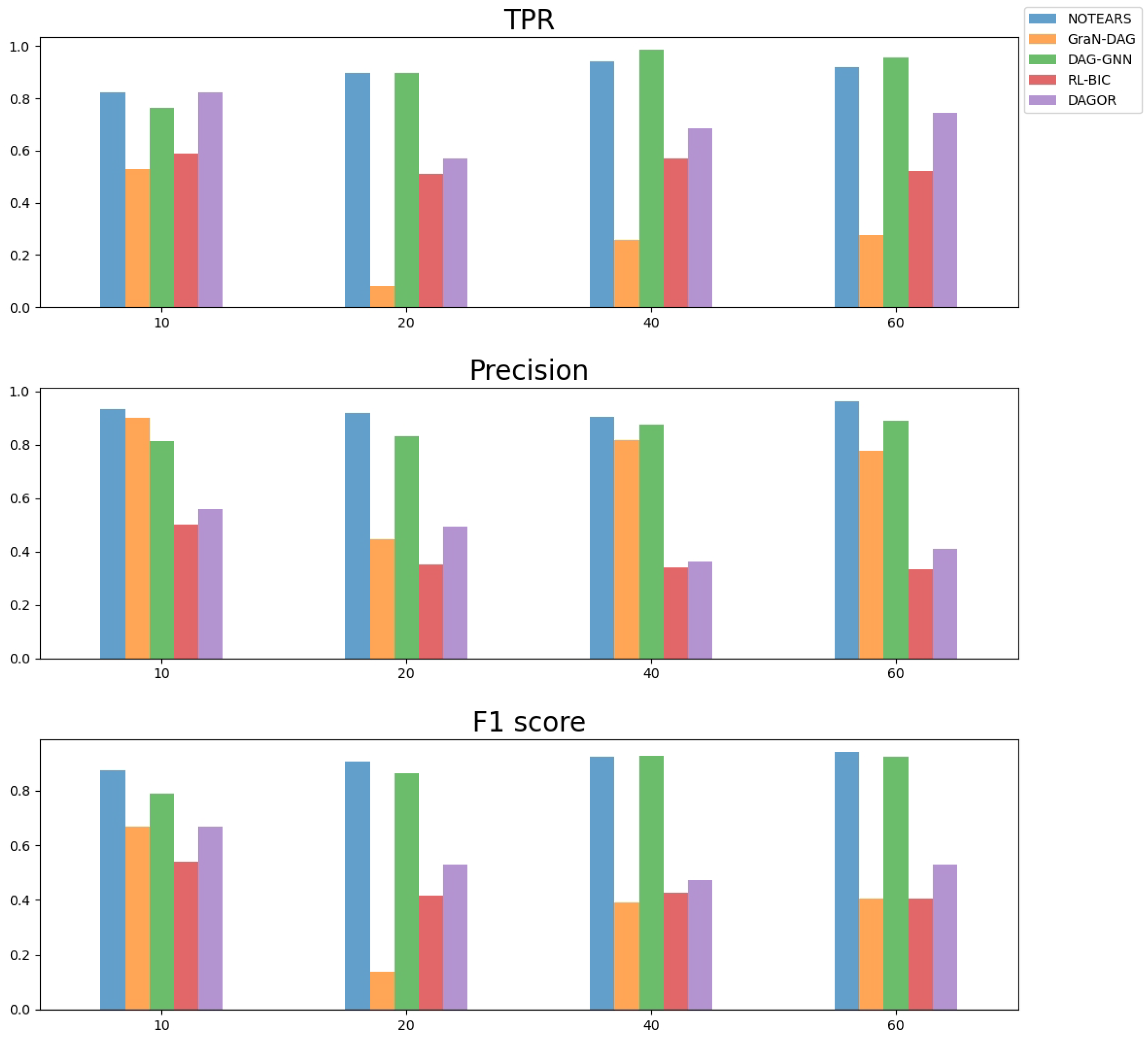
As presented in Figure 4, our method DAGOR has a really favorable performance on the non-linear synthetic MLP SEM SF2 datasets, and in particular, DAGOR shows a high level in TPR metrics. For the TPR metrics, our method DAGOR achieves better performance than the other four algorithms on all the different vertex datasets. But in terms of the precision, the performance of DAGOR is not that good. For example, DAGOR’s precision is lower than the other four algorithms at 40 and 60 vertices SF2 datasets. But for F1 score metrics, DAGOR performs generally well, which means the DAGs learning ability of DAGOR is still promising.

In particular, the efficiency of our method DAGOR does not decrease obviously in the case of higher number of vertices in SF2. These results further prove that DAGOR can be used in discovering more realistic nonlinear causal relationships.

5.3. Benchmark Datasets Experiments

We also demonstrate the DAGOR model on four discrete real datasets: SARCH, INSURANCE, ALARM, and HAILFINDER.

Table 2. The statistics of the benchmark datasets.

Datasets	Vertices	Edges	Average Degree	Maximum in-Degree
SACHS	11	17	3.09	3
INSURANCE	27	52	3.75	3
ALARM	37	46	2.49	4
HAILFINDER	56	2656	3.54	4

describes the details about four datasets.

The results in

Table 3. BIC scores of the algorithms on benchmark datasets.

Datasets	NOTEARS	GraN-DAG	DAG-GNN	RL-BIC	DAGOR
SACHS	−89,689.1890	−91,492.0830	−80,400.6366	−75,755.7475	−73,393.3803
INSURANCE	−172,398.5148	−209,095.8312	−215,748.3429	−142,541.3019	−132,670.8996
ALARM	−149,468.1578	−195,862.0969	−125,510.0427	−106,664.5271	−96,735.5799
HAILFINDER	−559,955.9584	−645,828.4366	−577,215.7237	−559,604.4484	−469,238.9180

show our model’s DAGs structure attains a superior BIC score comparing with the other four alternative methods, which means our method is effective on these four real datasets.

In addition, the results in

Table 4. BDeu scores of the algorithms on benchmark datasets.

Datasets	NOTEARS	GraN-DAG	DAG-GNN	RL-BIC	DAGOR
SACHS	−89,682.8663	−91,488.9172	−80,341.4775	−75,575.0589	−73,235.1207
INSURANCE	−172,332.5778	−209,095.8312	−215,809.0844	−142,083.4768	−131,250.0165
ALARM	−149,468.1578	−195,980.7651	−125,224.9439	−105,564.1670	−95,107.4008
HAILFINDER	−557,558.2384	−645,312.3031	−574,989.1839	−549,179.3662	−464,266.7738

further prove the findings, where the BDeu score of DAGOR exhibiting superiority over other methods. This outperformance reflects the effectiveness of our model in structure learning to the causality of the discrete real data.

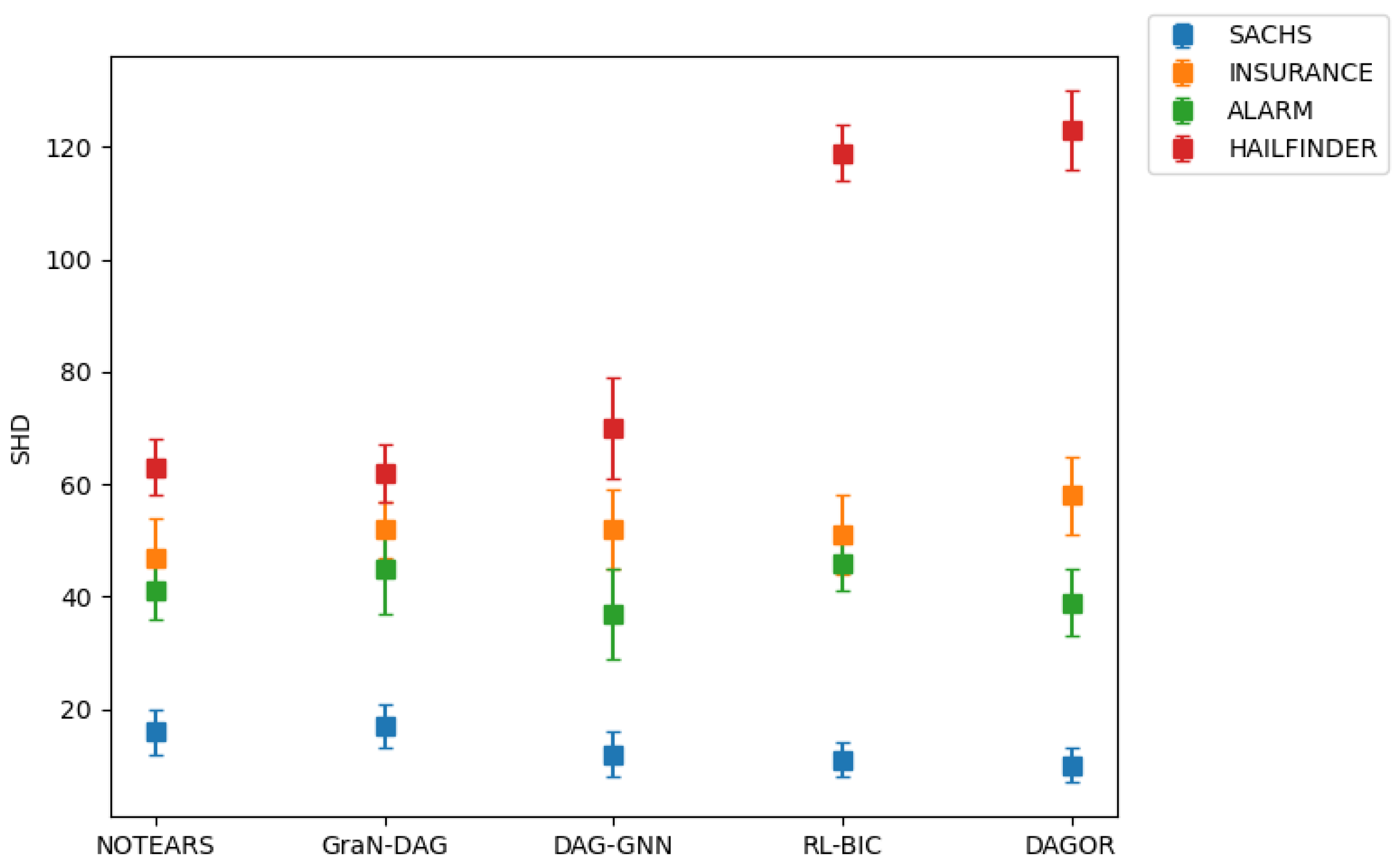
Furthermore, Figure 5 shows the results of the Structural Hamming distances associated with DAGs learnt by various methods across the four benchmark datasets. We find that DAGOR can perform well on SACHS, INSURANCE and ALARM, but the performance on HAILFINDER is worse than other algorithms, which suggests that DAGOR fails to get a good structure when dealing with very large networks. However, most real world networks do not have such large vertices and edges, which means using our DAGOR is enough in most cases.

6. Conclusions

In this study, we introduce a new method for learning directed acyclic graphs named DAGOR, which based on the combination of topological sorts and QR factorization. Firstly, we establish topological sorts through matrix congruent transformations applied to adjacency matrices. Next, the subsequent step involves QR factorization of the adjacency matrix with the obtained topological sorts. Leveraging the upper triangular properties of the decomposed matrix, we construct a least-square penalty function, which serves as a set of constraints for optimization. This innovative DAGs learning optimization strategy is integrated into a graph autoencoder network, where the Evidence Lower Bound serves as the training optimization objective. The performance of DAGOR is tested through extensive experiments conducted on both discrete and continuous datasets, which show its robust generalization capabilities and stability across diverse data modalities. These results demonstrate the potential of DAGOR as an effective tool for DAGs learning.