A Forward–Backward–Forward Algorithm for Quasi-Variational Inequalities in the Moving Set Case

Abstract

This paper addresses the challenge of solving quasi-variational inequalities (QVIs) by developing and analyzing a forward–backward–forward algorithm from a continuous and iterative perspective. QVIs extend classical variational inequalities by allowing the constraint set to depend on the decision variable, a formulation that is particularly useful in modeling various problems. A critical computational challenge in these settings is the expensive nature of projection operations, especially when closed-form solutions are unavailable. To mitigate this, we consider the moving set case and propose a forward–backward–forward algorithm that requires only one projection per iteration. Under the assumption that the operator is strongly monotone, we establish that the continuous trajectories generated by the corresponding dynamical system converge exponentially to the unique solution of the QVI. We extend Tseng’s well-known forward–backward–forward algorithm for variational inequalities by adapting it to the more complex framework of QVIs. We prove that it converges when applied to strongly monotone QVIs and derive its convergence rate. We perform numerical implementations of our proposed algorithm and give numerical comparisons with other related gradient projection algorithms for quasi-variational inequalities in the literature.

1. Introduction

Variational inequalities (VIs) have played an important role in mathematical optimization, providing a framework for modeling equilibrium conditions in diverse applications such as convex Nash games, traffic flow, and economic markets; see [1,2,3]. In the classical VI setting, the problem involves finding a point $x^{*}\in C$ within a fixed, non-empty, convex, and closed subset of a Euclidean space E such that

$$⟨F\left(x^{*}\right),z-x^{*}⟩\ge 0,\forall z\in C,$$

where $F:E\to E$ is a given operator. This approach has proven effective across many fields, including game theory, mechanics, stochastic systems, and hydrodynamics. However, the assumption that the constraint set C remains static can be overly restrictive when addressing the dynamic and evolving nature of many real-world problems.

To overcome this limitation, the concept of quasi-variational inequalities (QVIs) has been introduced [4,5,6]. QVIs extend the classical framework by allowing the constraint set to depend on the decision variable. More formally, the fixed set C is replaced by a set-valued mapping $C:E\to 2^E$, where for every $x\in E$, the corresponding set $C\left(x\right)$ is non-empty, closed, and convex. This yields the following QVI: find $x^{*}\in C\left(x^{*}\right)$ such that

$$⟨F\left(x^{*}\right),z-x^{*}⟩\ge 0,\forall z\in C\left(x^{*}\right).$$

(1)

This modification facilitates the modeling of complex interdependencies—such as those encountered in generalized Nash equilibrium scenarios with shared resources—thereby offering a more realistic representation across various fields, including transportation network equilibria, engineering, electricity market models, and dynamic traffic assignment [7,8,9,10,11,12].

Despite the superficial resemblance between VIs and QVIs, their underlying theories differ significantly. While the VI framework is supported by a comprehensive body of literature addressing solution existence, uniqueness, and algorithmic strategies, the theoretical development and computational methods for QVIs remain relatively underdeveloped. For the recent applications, numerical methods, and other aspects of QVIs, see [13,14,15,16,17,18,19,20,21,22,23,24,25,26,27,28,29,30,31,32,33].

A critical challenge in designing efficient algorithms for both VIs and QVIs is reducing the number of projection operations performed during each iteration. Projections can be computationally expensive, particularly when closed-form solutions are unavailable. In this work, we address this issue by associating a dynamical system of forward–backward–forward type with the QVI formulation. We then perform a convergence analysis of the trajectories generated by this dynamical system under the assumption that F is strongly monotone, showing that these trajectories converge exponentially to the unique solution of the QVIs.

This approach builds on earlier studies—most notably by Banert and Bot (see [34])—who examined continuous trajectories for locating zeros of the sum of a maximally monotone operator and a Lipschitz continuous monotone operator. By discretizing time explicitly, this framework naturally leads to Tseng’s forward–backward–forward algorithm with relaxation parameters (see [35]). The forward–backward–forward method for solving VIs has been extensively discussed in the literature; see, for instance [32,36,37,38,39,40,41]. In our work, we adapt these ideas for the more complex setting of QVIs.

Among the various formulations of QVIs, the moving set scenario is by far the most extensively studied. In this case, the constraint set is expressed as

$$C\left(x\right)=c\left(x\right)+C_0,$$

(2)

where $C_0$ is a fixed set and $c\left(x\right)$ is a function that captures the non static aspect of the constraints. This formulation strikes a balance between modeling flexibility and analytical tractability. In [13,15,16,18,23,24,25,26,42], methods for solving QVIs in the moving set case have been considered.

Through this study, we aim to contribute to the burgeoning field of QVIs by providing both theoretical insights and practical algorithmic solutions that bridge the gap between traditional VIs and their more flexible quasi-variational counterparts.

Outline of the Paper

In Section 2, we recall some basic facts, concepts, and lemmas, which are needed in the convergence analysis. Section 3 introduces the dynamical system of the forward–backward–forward type and carries out a convergence analysis for the generated trajectories to the unique solution of the QVI. In Section 4, we adapt Tseng’s forward–backward–forward algorithm for QVIs, prove the convergence, and derive the rate of convergence. Section 5 discusses the numerical implementations of the proposed algorithm with comparisons with other related algorithms. In Section 6, we summarize our key findings and propose directions for future research.

2. Preliminaries

In this section, we begin by establishing the key notations, followed by outlining the definitions, assumptions, and crucial lemmas necessary for our convergence analysis.

Throughout the article, $\parallel ·\parallel$ denotes the Euclidean vector norm and $⟨·,·⟩$ is the corresponding scalar product. ${\mathcal{P}}_C\left(x\right)$ is the projection of x onto the set C, i.e., 

$$\mathcal{P}\left(x\right)={\mathrm{argmin}}_{y\in C}\parallel y-x\parallel .$$

Here, we will focus on the operator $F:E\to E$. If the operator F is the gradient of a function f, then the VI can be understood as a necessary condition for optimality when minimizing f over the set C, and the QVI becomes a necessary condition for minimization with coupled constraints. In this article, we consider the operator F which is L-Lipschitz continuous, i.e.,

$$\parallel F\left(x\right)-F\left(y\right)\parallel \le L\parallel x-y\parallel ,\forall x,y\in E.$$

and $\mu$-strongly monotone, i.e.,

$$⟨F\left(x\right)-F\left(y\right),x-y⟩\ge {\mu \parallel x-y\parallel }^2,\forall x,y\in E.$$

If $\mu =0$, then F is a monotone operator. In this article, we always assume $\mu >0$. From the definitions above, it is trivial to deduce that $\mu \le L$.

By applying Theorem 4.3.5 from [43] to the operator F, we obtain the following corollary, which we will use in the study of convergence of our method.

Corollary 1.

Let $C\subset E$ be a convex set with $\mathrm{int}C\ne \varnothing$ and operator $F:C\to E$. Operator F is strongly monotone with parameter $\mu >0$ and Lipschitz continuous with Lipschitz constant $L>0$ if and only if

$${\parallel F\left(x\right)-F\left(y\right)\parallel }^2+\mu L{\parallel x-y\parallel }^2\le (L+\mu )⟨F\left(x\right)-F\left(y\right),x-y⟩,\forall x,y\in C.$$

(3)

Assumption 1.

Operator $F:E\to E$ is L-Lipschitz continuous and μ-strongly monotone.

In our analysis, the following lemma for projection mappings is used.

Lemma 1.

Let C be a closed convex set in E. Then, for a given $z\in E$, $u\in C$ satisfies

$$u={\mathcal{P}}_C\left(z\right),$$

if and only if

$$⟨u-z,v-u⟩\ge 0,\forall v\in C.$$

The primary challenge in developing algorithms for solving QVIs lies in the dynamic nature of the constraint set, which evolves during iterations; hence, ensuring that $C\left(x\right)$ does not change drastically as x varies is crucial, a requirement met by imposing a contractiveness condition on the projection operator. Moreover, one effective approach for establishing existence results for QVIs is to reformulate the problem into a fixed-point problem: $x^{*}\in C\left(x^{*}\right)$ is a solution of problem (1) if and only if

$$x^{*}=P_{C\left(x^{*}\right)}(x^{*}-\alpha F\left(x^{*}\right)),\alpha >0.$$

The existence theorem for solutions highlights a key distinction between VIs and QVIs. Specifically, if the operator F is strongly monotone and Lipschitz continuous over a closed and convex set, the VI admits a unique solution. However, in addition to these assumptions, the following assumption is crucial for convergence in QVI problems and is present in all existing results, indicating its necessity for current approaches [44,45]: there exists $l>0$ such that

$$\parallel P_{C\left(x\right)}\left(z\right)-P_{C\left(y\right)}\left(z\right)\parallel \le l\parallel x-y\parallel ,l<{\displaystyle \frac{\mu }{L}},\forall x,y,z\in E.$$

(4)

As we mentioned, in many important applications, the convex-valued set $C\left(x\right)$ is of the form (2). In this case,

$${\mathcal{P}}_{C\left(x\right)}\left(u\right)={\mathcal{P}}_{c\left(x\right)+C_0}\left(u\right)=c\left(x\right)+{\mathcal{P}}_{C_0}(u-c\left(x\right)),\forall x,u\in E.$$

If c is l-Lipschitz continuous, then

$$\begin{array}{ccc}\hfill \parallel {\mathcal{P}}_{C\left(x\right)}\left(u\right)-{\mathcal{P}}_{C\left(y\right)}{\left(u\right)\parallel }^2& =& \parallel c\left(x\right)+{\mathcal{P}}_{C_0}(u-c\left(x\right))-c\left(y\right)-{\mathcal{P}}_{C_0}{(u-c\left(y\right))\parallel }^2\hfill \\ & =& {\parallel c\left(x\right)-c\left(y\right)\parallel }^2+{\parallel {\mathcal{P}}_{C_0}(u-c\left(x\right))-{\mathcal{P}}_{C_0}(u-c\left(y\right))\parallel }^2\hfill \\ & & +2⟨c\left(x\right)-c\left(y\right),{\mathcal{P}}_{C_0}(u-c\left(x\right))-{\mathcal{P}}_{C_0}(u-c\left(y\right))⟩.\hfill \end{array}$$

Since,

$$\begin{array}{ccc}& & ⟨c\left(x\right)-c\left(y\right),{\mathcal{P}}_{C_0}(u-c\left(x\right))-{\mathcal{P}}_{C_0}(u-c\left(y\right))⟩\le \hfill \\ & & ⟨{\mathcal{P}}_{C_0}(u-c\left(y\right))-(u-c\left(x\right)),{\mathcal{P}}_{C_0}(u-c\left(x\right))-{\mathcal{P}}_{C_0}(u-c\left(y\right))⟩\hfill \\ & & \le -\parallel {\mathcal{P}}_{C_0}(u-c\left(x\right))-{\mathcal{P}}_{C_0}{(u-c\left(y\right))\parallel }^2,\hfill \end{array}$$

it follows

$$\begin{array}{c}\hfill \parallel {\mathcal{P}}_{C\left(x\right)}\left(u\right)-{\mathcal{P}}_{C\left(y\right)}{\left(u\right)\parallel }^2\le {\parallel c\left(x\right)-c\left(y\right)\parallel }^2\le l^2{\parallel x-y\parallel }^2.\end{array}$$

This shows that in the case of moving set, (4) holds if $l<{\displaystyle \frac{\mu }{L}}$, and our assumption is as follows.

Assumption 2.

$C:E\to 2^E$ is a set-valued mapping of the form $C\left(x\right)=c\left(x\right)+C_0$, $x\in E$, where $C_0\subset E$ is a non-empty closed convex set with $\mathrm{int}{C}_0\ne \varnothing$, and $c:E\to E$ is an l-Lipschitz continuous function such that $l<\mu /L$.

Let us note that, from Assumptions 1 and 2, it follows that there exists a unique solution $x^{*}\in C\left(x^{*}\right)$ of the problem (1), since the conditions of the theorems in [44,45] are satisfied.

3. A Dynamical System of Forward–Backward–Forward Type

In this section, we will analyze the trajectory generated by the following forward–backward–forward dynamical system for solving QVIs:

$$\begin{array}{ccc}\hfill y\left(t\right)& =& {\mathcal{P}}_{C\left(x\right(t\left)\right)}(x\left(t\right)-\alpha F\left(x\left(t\right)\right))\hfill \end{array}$$

(5)

$$\begin{array}{ccc}\hfill \dot{x}\left(t\right)+x\left(t\right)& =& y\left(t\right)+\alpha \left(F\right(x\left(t\right))-F(y\left(t\right)\left)\right)\hfill \\ \hfill x\left(0\right)& =& x_0,\hfill \end{array}$$

(6)

where $\alpha >0$ is a parameter of the method and $x_0\in E$. The formulation of this method has its roots in [38], where the continuous forward–backward–forward algorithm has been considered for solving VIs.

In the following, we will investigate the asymptotic behavior of the trajectory generated by the dynamical system (5) and (6).

Theorem 1.

Let $x\left(t\right)$ be a trajectory generated by the forward–backward–forward method (5) and (6). If Assumptions 1 and 2 hold and the conditions

$$0<\alpha <\min \left\{{\displaystyle \frac{2l(L+\mu )}{2L\mu -l^2{(L+\mu )}^2}},{\displaystyle \frac{1}{\sqrt{2}L}}\right\},$$

$${\displaystyle \frac{\alpha L}{1-2{\alpha }^2{L}^2}}\left({\displaystyle \frac{2\mu }{L+\mu }}+\sqrt{2(1-2{\alpha }^2{L}^2)}\right)<1-{\displaystyle \frac{l}{2}}$$

are satisfied, then $x\left(t\right)$ converges to the unique solution $x^{*}\in C\left(x^{*}\right)$ of (1) with exponential rate

$$\parallel x\left(t\right)-x^{*}\parallel \le e^{A_1\left(\alpha \right)t}\parallel x_0-x^{*}\parallel ,$$

where $A_1\left(\alpha \right)={\displaystyle \frac{l}{2}}+{\displaystyle \frac{\alpha l^2(L+\mu )}{4}}-{\displaystyle \frac{\alpha L\mu }{2(L+\mu )}}$. Furthermore,

$$\underset{t\to \infty }{\lim }\parallel \dot{x}\left(t\right)\parallel =0.$$

Proof. 

System (5) and (6) is an autonomous system of the type $\dot{x}=g\left(x\right)$, where

$$g\left(x\right)={\mathcal{P}}_{C\left(x\right)}(x-\alpha F\left(x\right))+\alpha \left(F\left(x\right)-F\left({\mathcal{P}}_{C\left(x\right)}(x-\alpha F\left(x\right))\right)\right)-x.$$

Since operator F is Lipschitz continuous and condition (4) is satisfied, function $g(·)$ is Lipschitz continuous. Indeed,

$$\begin{array}{ccc}\hfill \parallel g\left(x\right)-g\left(z\right)\parallel & \le & \parallel x-z\parallel +\alpha \parallel F\left(x\right)-F\left(z\right)\parallel \hfill \\ & & +\parallel {\mathcal{P}}_{C\left(x\right)}(x-\alpha F\left(x\right))-{\mathcal{P}}_{C\left(z\right)}(z-\alpha F\left(z\right))\parallel \hfill \\ & & +\alpha \parallel F\left({\mathcal{P}}_{C\left(x\right)}(x-\alpha F\left(x\right))\right)-F\left({\mathcal{P}}_{C\left(z\right)}(z-\alpha F\left(z\right))\right)\parallel \hfill \\ & \le & \parallel x-z\parallel +\alpha L\parallel x-z\parallel \hfill \\ & & +(1+\alpha L)\parallel {\mathcal{P}}_{C\left(x\right)}(x-\alpha F\left(x\right))-{\mathcal{P}}_{C\left(x\right)}(z-\alpha F\left(z\right))\hfill \\ & & +{\mathcal{P}}_{C\left(x\right)}(z-\alpha F\left(z\right))-{\mathcal{P}}_{C\left(z\right)}(z-\alpha F\left(z\right))\parallel \hfill \\ & \le & \parallel x-z\parallel +\alpha L\parallel x-z\parallel \hfill \\ & & +(1+\alpha L)(\parallel x-z\parallel +\alpha L\parallel x-z\parallel +l\parallel x-z\parallel )\hfill \\ & & =(2+l+3\alpha L+l\alpha L+{\alpha }^2{L}^2)\parallel x-z\parallel .\hfill \end{array}$$

Then, the classical Cauchy–Lipschitz–Picard theorem ensures the existence and uniqueness of the trajectory $x\in C^1([0,+\infty ),E)$ associated with (5) and (6). Also, note that the conditions of the theorem guarantee the existence and uniqueness of the solution $x^{*}\in C\left(x^{*}\right)$ to QVI (1). Let us prove that the trajectory $x\left(t\right)$, $t\ge 0$ generated by (5) and (6) converges exponentially to $x^{*}$.

Equation (5) can be written as

$$y\left(t\right)=c\left(x\left(t\right)\right)+{\mathcal{P}}_{C_0}(x\left(t\right)-\alpha F\left(x\left(t\right)\right)-c\left(x\left(t\right)\right)).$$

From here, we can see that $y\left(t\right)-c\left(x\left(t\right)\right)\in C_0$. Using this and Lemma 1, we obtain

$$⟨y\left(t\right)-x\left(t\right)+\alpha F\left(x\left(t\right)\right),w-y\left(t\right)+c\left(x\left(t\right)\right)⟩\ge 0,\forall w\in C_0.$$

Substituting $w=x^{*}-c\left(x^{*}\right)\in C_0$ into the inequality above, we get

$$⟨y\left(t\right)-x\left(t\right)+\alpha F\left(x\left(t\right)\right),x^{*}-y\left(t\right)+c\left(x\left(t\right)\right)-c\left(x^{*}\right)⟩\ge 0.$$

(7)

From (6), we conclude $y\left(t\right)=\dot{x}\left(t\right)+x\left(t\right)-\alpha (F\left(x\left(t\right)\right)-F\left(y\left(t\right)\right))$. Then, (7) becomes

$$⟨\dot{x}\left(t\right)+\alpha F\left(y\left(t\right)\right),x^{*}-y\left(t\right)+c\left(x\left(t\right)\right)-c\left(x^{*}\right)⟩\ge 0.$$

(8)

From (5), we see that $y\left(t\right)\in C\left(x\right(t\left)\right)$, so $y\left(t\right)-c\left(x\left(t\right)\right)\in C_0$. Now, substituting $z=c\left(x^{*}\right)+y\left(t\right)-c\left(x\left(t\right)\right)\in c\left(x^{*}\right)+C_0=C\left(x^{*}\right)$ into (1) and multiplying by $\alpha >0$, we obtain

$$\alpha ⟨F\left(x^{*}\right),y\left(t\right)-x^{*}+c\left(x^{*}\right)-c\left(x\left(t\right)\right)⟩\ge 0.$$

(9)

By combining inequalities (8) and (9), we have

$$⟨\dot{x}\left(t\right)+\alpha (F\left(y\left(t\right)\right)-F\left(x^{*}\right)),x^{*}-y\left(t\right)+c\left(x\left(t\right)\right)-c\left(x^{*}\right)⟩\ge 0,$$

which is equivalent to

$$\begin{array}{ccc}& & ⟨\dot{x}\left(t\right),x^{*}-x\left(t\right)⟩+⟨\dot{x}\left(t\right),x\left(t\right)-y\left(t\right)⟩+⟨\dot{x}\left(t\right),c\left(x\left(t\right)\right)-c\left(x^{*}\right)⟩\hfill \\ & & +\alpha ⟨F\left(y\left(t\right)\right)-F\left(x^{*}\right),x^{*}-y\left(t\right)⟩+\alpha ⟨F\left(y\left(t\right)\right)-F\left(x^{*}\right),c\left(x\left(t\right)\right)-c\left(x^{*}\right)⟩\ge 0.\hfill \end{array}$$

Let us note that the following obvious equalities hold:

$$⟨\dot{x}\left(t\right),\dot{x}\left(t\right)⟩={\parallel \dot{x}\left(t\right)\parallel }^2,$$

$$⟨\dot{x}\left(t\right),x\left(t\right)-x^{*}⟩={\displaystyle \frac{1}{2}}{\displaystyle \frac{\mathrm{d}}{\mathrm{d}t}}\left(\parallel x\left(t\right)-x^{*}{\parallel }^2\right).$$

Now, we have

$$\begin{array}{ccc}\hfill {\displaystyle \frac{1}{2}}{\displaystyle \frac{\mathrm{d}}{\mathrm{d}t}}\left(\parallel x\left(t\right)-x^{*}{\parallel }^2\right)& \le & ⟨\dot{x}\left(t\right),c\left(x\left(t\right)\right)-c\left(x^{*}\right)⟩-{\parallel \dot{x}\left(t\right)\parallel }^2\hfill \\ & +& \alpha ⟨\dot{x}\left(t\right),F\left(x\left(t\right)\right)-F\left(y\left(t\right)\right)⟩+\alpha ⟨F\left(y\left(t\right)\right)-F\left(x^{*}\right),x^{*}-y\left(t\right)⟩\hfill \\ & +& \alpha ⟨F(y\left(t\right)-F\left(x^{*}\right),c\left(x\left(t\right)\right)-c\left(x^{*}\right)⟩.\hfill \end{array}$$

(10)

In what follows, we shall estimate each term of the previously stated sum.

Using the Peter-Paul inequality, the l-Lipschitz continuity of c, and the L-Lipschitz continuity of F, we obtain

$$\begin{array}{ccc}\hfill ⟨\dot{x}\left(t\right),c\left(x\left(t\right)\right)-c\left(x^{*}\right)⟩& \le & {\displaystyle \frac{l}{2}}\parallel \dot{x}{\left(t\right)\parallel }^2+{\displaystyle \frac{l}{2}}{\parallel x\left(t\right)-x^{*}\parallel }^2,\hfill \\ \hfill \alpha ⟨\dot{x}\left(t\right),F\left(x\left(t\right)\right)-F\left(y\left(t\right)\right)⟩& \le & {\displaystyle \frac{\alpha \gamma }{2}}\parallel \dot{x}{\left(t\right)\parallel }^2+{\displaystyle \frac{\alpha L^2}{2\gamma }}{\parallel x\left(t\right)-y\left(t\right)\parallel }^2,(\gamma >0),\hfill \\ \hfill \alpha ⟨F(y\left(t\right)-F\left(x^{*}\right),c\left(x\left(t\right)\right)-c\left(x^{*}\right)⟩& \le & {\displaystyle \frac{\alpha }{L+\mu }}\parallel F\left(y\left(t\right)\right)-F\left(x^{*}\right){\parallel }^2+{\displaystyle \frac{\alpha l^2(L+\mu )}{4}}{\parallel x\left(t\right)-x^{*}\parallel }^2.\hfill \end{array}$$

(11)

From Assumptions 1 and 2, it follows that the conditions from Corollary 1 are satisfied, so inequality (3) holds. Hence,

$$\alpha ⟨F\left(y\left(t\right)\right)-F\left(x^{*}\right),x^{*}-y\left(t\right)⟩\le -{\displaystyle \frac{\alpha }{L+\mu }}\parallel F\left(y\left(t\right)\right)-F\left(x^{*}\right){\parallel }^2-{\displaystyle \frac{\alpha L\mu }{L+\mu }}\parallel y\left(t\right)-x^{*}\parallel .$$

Inserting the obtained inequalities in (10), we get

$$\begin{array}{ccc}& & {\displaystyle \frac{1}{2}}{\displaystyle \frac{\mathrm{d}}{\mathrm{d}t}}\left(\parallel x\left(t\right)-x^{*}{\parallel }^2\right)+\left(1-{\displaystyle \frac{l}{2}}-{\displaystyle \frac{\alpha \gamma }{2}}\right)\parallel \dot{x}{\left(t\right)\parallel }^2\le \left({\displaystyle \frac{l}{2}}+{\displaystyle \frac{\alpha l^2(L+\mu )}{4}}\right){\parallel x\left(t\right)-x^{*}\parallel }^2\hfill \\ & & +{\displaystyle \frac{\alpha L^2}{2\gamma }}{\parallel x\left(t\right)-y\left(t\right)\parallel }^2-{\displaystyle \frac{\alpha L\mu }{L+\mu }}{\parallel y\left(t\right)-x^{*}\parallel }^2.\hfill \end{array}$$

Let us estimate $\parallel y\left(t\right)-x^{*}\parallel$ in terms of $\parallel x\left(t\right)-x^{*}\parallel$ and $\parallel x\left(t\right)-y\left(t\right)\parallel$.

$$\begin{array}{ccc}\hfill \parallel y\left(t\right)-x^{*}{\parallel }^2& =& {\parallel y\left(t\right)-x\left(t\right)\parallel }^2+{\parallel x\left(t\right)-x^{*}\parallel }^2+2⟨y\left(t\right)-x\left(t\right),x\left(t\right)-x^{*}⟩\hfill \\ & \ge & {-\parallel y\left(t\right)-x\left(t\right)\parallel }^2+{\displaystyle \frac{1}{2}}{\parallel x\left(t\right)-x^{*}\parallel }^2.\hfill \end{array}$$

Now, we have

$$\begin{array}{ccc}& & {\displaystyle \frac{1}{2}}{\displaystyle \frac{\mathrm{d}}{\mathrm{d}t}}\left(\parallel x\left(t\right)-x^{*}{\parallel }^2\right)+\left(1-{\displaystyle \frac{l}{2}}-{\displaystyle \frac{\alpha \gamma }{2}}\right)\parallel \dot{x}{\left(t\right)\parallel }^2\le \left({\displaystyle \frac{\alpha L^2}{2\gamma }}+{\displaystyle \frac{\alpha L\mu }{L+\mu }}\right){\parallel x\left(t\right)-y\left(t\right)\parallel }^2\hfill \\ & & +\left({\displaystyle \frac{l}{2}}+{\displaystyle \frac{\alpha l^2(L+\mu )}{4}}-{\displaystyle \frac{\alpha L\mu }{2(L+\mu )}}\right){\parallel x\left(t\right)-x^{*}\parallel }^2.\hfill \end{array}$$

Similarly, we will derive an estimation for $\parallel x\left(t\right)-y\left(t\right)\parallel$ in terms of $\parallel \dot{x}\left(t\right)\parallel$.

$$\begin{array}{ccc}\hfill {\parallel x\left(t\right)-y\left(t\right)\parallel }^2& =& \parallel -\dot{x}{\left(t\right)+\alpha (F\left(x\left(t\right)\right)-F\left(y\left(t\right)\right))\parallel }^2\hfill \\ & \le & \parallel \dot{x}{\left(t\right)\parallel }^2+{\alpha }^2{L}^2{\parallel x\left(t\right)-y\left(t\right)\parallel }^2-2⟨\dot{x}\left(t\right),\alpha (F\left(x\left(t\right)\right)-F\left(y\left(t\right)\right))⟩\hfill \\ & \le & 2\parallel \dot{x}{\left(t\right)\parallel }^2+2{\alpha }^2{L}^2{\parallel x\left(t\right)-y\left(t\right)\parallel }^2,\hfill \end{array}$$

hence,

$$\begin{array}{c}\hfill {\parallel x\left(t\right)-y\left(t\right)\parallel }^2\le {\displaystyle \frac{2}{1-2{\alpha }^2{L}^2}}{\parallel \dot{x}\left(t\right)\parallel }^2.\end{array}$$

Note that $1-2{\alpha }^2{L}^2>0$ holds due to the theorem’s conditions. Finally, from all of the above, we obtain the following estimate:

$$\begin{array}{ccc}& & {\displaystyle \frac{1}{2}}{\displaystyle \frac{\mathrm{d}}{\mathrm{d}t}}\left(\parallel \dot{x}\left(t\right)-x^{*}{\parallel }^2\right)+B_1\left(\alpha \right)\parallel \dot{x}{\left(t\right)\parallel }^2\le A_1\left(\alpha \right){\parallel x\left(t\right)-x^{*}\parallel }^2,\hfill \end{array}$$

(12)

where

$$B_1\left(\alpha \right)=1-{\displaystyle \frac{l}{2}}-{\displaystyle \frac{\alpha \gamma }{2}}-{\displaystyle \frac{2}{1-2{\alpha }^2{L}^2}}\left({\displaystyle \frac{\alpha L^2}{2\gamma }}+{\displaystyle \frac{\alpha L\mu }{L+\mu }}\right),$$

$$A_1\left(\alpha \right)={\displaystyle \frac{l}{2}}+{\displaystyle \frac{\alpha l^2(L+\mu )}{4}}-{\displaystyle \frac{\alpha L\mu }{2(L+\mu )}}.$$

Inequality (11) holds for all $\gamma >0$. We choose $\gamma$ so that the expression $B_1\left(\alpha \right)$ is maximized, i.e., 

$${\displaystyle \frac{\alpha \gamma }{2}}+{\displaystyle \frac{\alpha L^2}{\gamma (1-2{\alpha }^2{L}^2)}}\to \min .$$

This is achieved for $\gamma ={\displaystyle \frac{\sqrt{2}L}{\sqrt{1-2{\alpha }^2{L}^2}}}$. Now, $B_1\left(\alpha \right)$ becomes

$$B_1\left(\alpha \right)=1-{\displaystyle \frac{l}{2}}-{\displaystyle \frac{\alpha L}{1-2{\alpha }^2{L}^2}}\left({\displaystyle \frac{2\mu }{L+\mu }}+\sqrt{2(1-2{\alpha }^2{L}^2)}\right).$$

It follows from the conditions of the theorem that there exists a choice of $\alpha$ such that $B_1\left(\alpha \right)>0$ and $A_1\left(\alpha \right)<0$. More on this is presented after the end of the proof.

Since, $B_1\left(\alpha \right)>0$ it follows

$${\displaystyle \frac{1}{2}}{\displaystyle \frac{\mathrm{d}}{\mathrm{d}t}}\left(\parallel \dot{x}\left(t\right)-x^{*}{\parallel }^2\right)\le A_1\left(\alpha \right){\parallel x\left(t\right)-x^{*}\parallel }^2,$$

from which we obtain

$$\parallel x\left(t\right)-x^{*}{\parallel }^2\le A_0{e}^{2A_1\left(\alpha \right)t}.$$

Substituting the initial condition $x\left(0\right)=x_0$, we obtain $A_0={\parallel x_0-x^{*}\parallel }^2$, and finally we get that the trajectory $x\left(t\right)$ converges to the unique solution $x^{*}\in C\left(x^{*}\right)$:

$$\parallel x\left(t\right)-x^{*}\parallel \le e^{A_1\left(\alpha \right)t}\parallel x_0-x^{*}\parallel ,as t\to \infty .$$

In addition, integrating inequality (12) on $[0,T]$, we obtain

$${\displaystyle \frac{1}{2}}\parallel x\left(T\right)-x^{*}{\parallel }^2+{\displaystyle \frac{1}{2}}\parallel x_0-x^{*}{\parallel }^2+B_1\left(\alpha \right){\int }_0^T\parallel \dot{x}{\left(t\right)\parallel }^{2}dt\le A_1\left(\alpha \right){\int }_0^T{\parallel x\left(t\right)-x^{*}\parallel }^{2}dt\le 0.$$

From here, when $T\to +\infty$, we get

$$B_1\left(\alpha \right){\int }_0^{+\infty }\parallel \dot{x}{\left(t\right)\parallel }^{2}dt\le {\displaystyle \frac{1}{2}}{\parallel x_0-x^{*}\parallel }^2<\infty .$$

Having in mind that $B_1\left(\alpha \right)>0$, it follows that

$$\underset{t\to \infty }{\lim }\parallel \dot{x}{\left(t\right)\parallel }^2=0,i.e.,\underset{t\to \infty }{\lim }\parallel \dot{x}\left(t\right)\parallel =0.$$

This completes the proof of the theorem.    □

Remark 1.

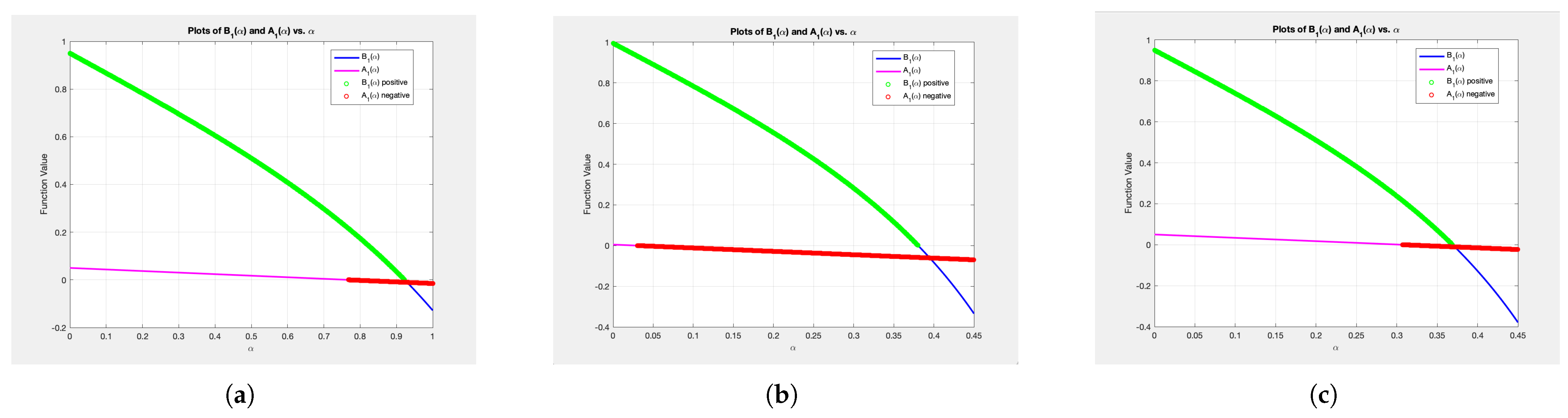
The conditions stated in the theorem appear to be quite complex, raising the question of whether there are any real situations in which these conditions are met. We will graphically illustrate some of the cases where the conditions of the theorem are satisfied (Figure 1).

Figure 1. The positive part of the graph of $B_1\left(\alpha \right)$ is in green and the negative part of the graph of $A_1\left(\alpha \right)$ is in red for: (a) $l=0.1,$ $L=0.4,$ $\mu =0.2$; (b) $l=0.01,$ $L=1,$ $\mu =0.5$; (c) $l=0.1,$ $L=1,$ $\mu =0.5$.

We have used the following parameters:

(a)

$l=0.1,$ $L=0.4,$ and $\mu =0.2$ for Graph 1;

(b)

$l=0.01,$ $L=1,$ and $\mu =0.5$ for Graph 2;

(c)

$l=0.1,$ $L=1,$ and $\mu =0.5$ for Graph 3.

The part of the graph for $B_1\left(\alpha \right)$ that is positive is marked in green, while the part of the graph for $A_1\left(\alpha \right)$ that is negative is marked in red. Clearly, we can find an interval for $\alpha$ where both conditions are satisfied.

4. A Forward–Backward–Forward Algorithm

In this section, we analyze the convergence of Tseng’s forward–backward–forward algorithm derived by the time discretization of the dynamical system (5) and (6) in the context of solving strongly monotone quasi-variational inequalities. The explicit time discretization of the dynamical system (5) and (6) with initial point $x_0\in E$ yields for every $n\ge 0$ the following equation:

$$x_{n+1}={\mathcal{P}}_{C\left(x_n\right)}(x_n-\alpha F\left(x_n\right))+\alpha F\left(x_n\right)-\alpha F\left({\mathcal{P}}_{C\left(x_n\right)}(x_n-\alpha F\left(x_n\right))\right).$$

Denoting $y_n={\mathcal{P}}_{C\left(x_n\right)}(x_n-\alpha F\left(x_n\right))$, we can rewrite this scheme as

$$\begin{array}{ccc}\hfill y_n& =& {\mathcal{P}}_{C\left(x_n\right)}(x_n-\alpha F\left(x_n\right))\hfill \end{array}$$

(13)

$$\begin{array}{ccc}\hfill x_{n+1}& =& y_n+\alpha (F\left(x_n\right)-F\left(y_n\right)),\hfill \end{array}$$

(14)

In the case $C\left(x\right)\equiv C$, for all $x\in E$, this iterative scheme reduces to the classical forward–backward–forward algorithm for solving variational inequalities as introduced in [35].

In the next table we present a forward-backward-forward algorithm (Algorithm 1) for solving QVI in the moving set case.

Algorithm 1 Forward-Backward-Forward Algorithm

Initialization: Choose the starting point $x_0\in E$ and the step size $\alpha >0$. Set $n=0$.

Step 1: Compute $y_n={\mathcal{P}}_{C\left(x_n\right)}(x_n-\alpha F\left(x_n\right))$.

If $y_n=x_n$ or $F\left(y_n\right)=0$, then STOP: $y_n$ is a solution.

Step 2: Set $x_{n+1}=y_n+\alpha (F\left(x_n\right)-F\left(y_n\right))$, update n to $n+1$ and go to Step 1.

For the convergence analysis, we assume that Algorithm 1 does not terminate after a finite number of iterations. In other words, we assume that for every $n\ge 0$, it holds that $x_n\ne y_n$ and $F\left(y_n\right)\ne 0$.

Since $C\left(x\right)=c\left(x\right)+C_0$, for all $x\in E$, equality (13) can be written in the form

$$y_n-c\left(x_n\right)={\mathcal{P}}_{C_0}(x_n-c\left(x_n\right)-\alpha F\left(x_n\right)).$$

According to Lemma 1, this can be rewritten as

$$⟨y_n-x_n+\alpha F\left(x_n\right),w-y_n+c\left(x_n\right)⟩\ge 0,\forall w\in C_0.$$

Let $w=x^{*}-c\left(x^{*}\right)\in C_0$, so

$$⟨y_n-x_n+\alpha F\left(x_n\right),x^{*}-y_n+c\left(x_n\right)-c\left(x^{*}\right)⟩\ge 0.$$

(15)

Since $x^{*}\in C\left(x^{*}\right)$ is a unique solution of quasi-variational inequality (1), then for every $z\in C\left(x^{*}\right)$, we have

$$⟨F\left(x^{*}\right),z-x^{*}⟩\ge 0.$$

Substituting $z=y_n-c\left(x_n\right)+c\left(x^{*}\right)\in C\left(x^{*}\right)$ into this inequality yields

$$⟨F\left(x^{*}\right),y_n-x^{*}-c\left(x_n\right)+c\left(x^{*}\right)⟩\ge 0.$$

(16)

Multiplying both sides of (16) by $\alpha >0$ and adding the resulting inequality to (15) yields

$$⟨y_n-x_n+\alpha (F\left(x_n\right)-F\left(x^{*}\right)),x^{*}-y_n+c\left(x_n\right)-c\left(x^{*}\right)⟩\ge 0.$$

From (14), it yields $y_n=x_{n+1}-\alpha (F\left(x_n\right)-F\left(y_n\right))$, so

$$⟨x_{n+1}-x_n+\alpha (F\left(y_n\right)-F\left(x^{*}\right)),x^{*}-y_n+c\left(x_n\right)-c\left(x^{*}\right)⟩\ge 0.$$

By expanding the terms and applying the properties of the scalar product, we obtain

$$\begin{array}{cc}\hfill & 2⟨x_{n+1}-x_n,x^{*}-x_n⟩+2⟨x_{n+1}-x_n,x_n-y_n⟩\hfill \\ \hfill & +2⟨x_{n+1}-x_n,c\left(x_n\right)-c\left(x^{*}\right)⟩+2\alpha ⟨F\left(y_n\right)-F\left(x^{*}\right),x^{*}-y_n⟩\hfill \\ \hfill & +2\alpha ⟨F\left(y_n\right)-F\left(x^{*}\right),c\left(x_n\right)-c\left(x^{*}\right)⟩\ge 0\hfill \end{array}$$

(17)

Using the identity for scalar products

$$2⟨u-v,u-w⟩={\parallel u-v\parallel }^2{+\parallel u-w\parallel }^2-{\parallel v-w\parallel }^2,\forall u,v,w\in E,$$

we get

$$2⟨x_{n+1}-x_n,x^{*}-x_n⟩=\parallel x_{n+1}-x_n{\parallel }^2+\parallel x_n-x^{*}{\parallel }^2-{\parallel x_{n+1}-x^{*}\parallel }^2,$$

$$2⟨x_{n+1}-x_n,x_n-y_n⟩=-\parallel x_{n+1}-x_n{\parallel }^2-\parallel x_n-y_n{\parallel }^2+{\parallel x_{n+1}-y_n\parallel }^2.$$

Since F is L-Lipschitz continuous, we have

$$\begin{array}{ccc}\hfill \parallel x_{n+1}-y_n{\parallel }^2& =& \parallel x_{n+1}-x_{n+1}+\alpha (F\left(x_n\right)-F\left(y_n\right)){\parallel }^2={\alpha }^2{\parallel F\left(x_n\right)-F\left(y_n\right)\parallel }^2\hfill \\ & \le & {\alpha }^2{L}^2{\parallel x_n-y_n\parallel }^2.\hfill \end{array}$$

By deriving analogous estimates as in the proof of the theorem for the dynamical system, we have

$$\begin{array}{ccc}\hfill ⟨x_{n+1}-x_n,c\left(x_n\right)-c\left(x^{*}\right)⟩& \le & {\displaystyle \frac{l}{2}}\parallel x_{n+1}-x_n{\parallel }^2+{\displaystyle \frac{l}{2}}{\parallel x_n-x^{*}\parallel }^2,\hfill \\ \hfill \alpha ⟨F\left(y_n\right)-F\left(x^{*}\right),c\left(x_n\right)-c\left(x^{*}\right)⟩& \le & {\displaystyle \frac{\alpha }{L+\mu }}\parallel F\left(y_n\right)-F\left(x^{*}\right){\parallel }^2+{\displaystyle \frac{\alpha l^2(L+\mu )}{4}}{\parallel x_n-x^{*}\parallel }^2.\hfill \\ \hfill \alpha ⟨F\left(y_n\right)-F\left(x^{*}\right),x^{*}-y_n⟩& \le & -{\displaystyle \frac{\alpha }{L+\mu }}\parallel F\left(y_n\right)-F\left(x^{*}\right){\parallel }^2-{\displaystyle \frac{\alpha L\mu }{L+\mu }}\parallel y_n-x^{*}\parallel .\hfill \end{array}$$

Substituting the obtained estimates yields

$$\begin{array}{ccc}\hfill \parallel x_{n+1}-x^{*}{\parallel }^2& \le & \left(1+l+{\displaystyle \frac{\alpha l^2(L+\mu )}{2}}\right)\parallel x_n-x^{*}{\parallel }^2+l{\parallel x_{n+1}-x_n\parallel }^2\hfill \\ & & +({\alpha }^2{L}^2-1)\parallel x_n-y_n{\parallel }^2-{\displaystyle \frac{2\alpha L\mu }{L+\mu }}{\parallel y_n-x^{*}\parallel }^2\hfill \end{array}$$

Furthermore, reasoning analogously to the continuous method, we obtain

$$\parallel y_n-x^{*}{\parallel }^2\ge -\parallel y_n-x_n{\parallel }^2+{\displaystyle \frac{1}{2}}{\parallel x_n-x^{*}\parallel }^2.$$

and

$$\parallel x_n-y_n{\parallel }^2=\parallel x_n-x_{n+1}+\alpha (F\left(x_n\right)-F\left(y_n\right)){\parallel }^2\le \parallel x_n-x_{n+1}{\parallel }^2+{\alpha }^2{L}^2{\parallel x_n-y_n\parallel }^2,$$

from which it follows that

$$\parallel x_n-y_n{\parallel }^2\le {\displaystyle \frac{2}{1-2{\alpha }^2{L}^2}}{\parallel x_{n+1}-x_n\parallel }^2,$$

assuming that $\alpha <{\left(\sqrt{2}L\right)}^{-1}$. Finally, we conclude that

$$\parallel x_{n+1}-x^{*}{\parallel }^2+B_2\left(\alpha \right)\parallel x_{n+1}-x_n{\parallel }^2\le A_2\left(\alpha \right){\parallel x_n-x^{*}\parallel }^2,$$

where

$$B_2\left(\alpha \right)={\displaystyle \frac{2}{1-2{\alpha }^2{L}^2}}\left(1-{\alpha }^2{L}^2-{\displaystyle \frac{2\alpha L\mu }{L+\mu }}\right)-l$$

and

$$A_2\left(\alpha \right)=1+l+{\displaystyle \frac{\alpha l^2(L+\mu )}{2}}-{\displaystyle \frac{\alpha L\mu }{L+\mu }}.$$

For the choice of $\alpha$ such that

$${\displaystyle \frac{2l(L+\mu )}{l^2{(L+\mu )}^2-2L\mu }}<\alpha <{\displaystyle \frac{\sqrt{\frac{L^2{\mu }^2}{{(L+\mu )}^2}+L^2(1-l)(1-\frac{l}{2})}-\frac{L\mu }{L+\mu }}{(1-l)L^2}}$$

we obtain that $B_2\left(\alpha \right)>0$ and $0<A_2\left(\alpha \right)<1$.

Thus, the following theorem is proven.

Theorem 2.

Let ${\left(x_n\right)}_{n\ge 0}$ be the iterates generated by Algorithm 1 using step-size $\alpha >0$ satisfying

$${\displaystyle \frac{2l(L+\mu )}{l^2{(L+\mu )}^2-2L\mu }}<\alpha <\min \left\{{\displaystyle \frac{\sqrt{\frac{L^2{\mu }^2}{{(L+\mu )}^2}+L^2(1-l)(1-\frac{l}{2})}-\frac{L\mu }{L+\mu }}{(1-l)L^2}},{\left(\sqrt{2}L\right)}^{-1}\right\}.$$

Suppose Assumptions 1 and 2 hold. Then, for any $n\ge 0$, we have

$$\parallel x_{n+1}-x^{*}{\parallel }^2\le C_2^{n+1}\left(\alpha \right){\parallel x_0-x^{*}\parallel }^2,$$

and $\parallel x_{n+1}-x_n\parallel \to 0$ as $n\to \infty$.

Remark 2.

By discretizing the dynamical system (5) and (6), we can form a forward–backward–forward iterative algorithm with relaxation parameters as follows:

$${\displaystyle \frac{x_{n+1}-x_n}{h_n}}+x_n={\mathcal{P}}_{C\left(x_n\right)}(x_n-\alpha F\left(x_n\right))+\alpha F\left(x_n\right)-\alpha F\left({\mathcal{P}}_{C\left(x_n\right)}(x_n-\alpha F\left(x_n\right))\right).$$

Denoting $y_n={\mathcal{P}}_{C\left(x_n\right)}(x_n-\alpha F\left(x_n\right))$, we can rewrite this scheme as

$$\begin{array}{ccc}\hfill y_n& =& {\mathcal{P}}_{C\left(x_n\right)}(x_n-\alpha F\left(x_n\right))\hfill \\ \hfill x_{n+1}& =& h_n(y_n+\alpha (F\left(x_n\right)-F\left(y_n\right)))-(1-h_n)x_n,\hfill \end{array}$$

where ${\left(h_n\right)}_{n\ge 0}$ are relaxation parameters. Here, convergence has been proven and a convergence estimate has been derived for $h_n\equiv 1$. Establishing convergence for an arbitrary sequence $\left(h_n\right)$ presents a promising direction for further research.

5. Numerical Experiments

In this section, we present a numerical experiment which we carried out in order to compare Algorithm 1 with other algorithms in the literature designed for solving quasi-variational inequalities. We implemented the numerical codes in Matlab and performed all computations on a Windows desktop with an Acer laptop with Intel(R) Core(TM) i5-6300U processor (Acer Inc., New Taipei City, Taiwan) at 2.40 gigahertz.

Let there be a QVI such that

$$C_0=\{x\in {\mathbb{R}}^4:\parallel x\parallel =d\},$$

$$c\left(x\right)=lx,$$

and

$$F:{\mathbb{R}}^4\to {\mathbb{R}}^4,F\left(x\right)=\left(\sqrt{x_1^2+x_2^2}-1,\sqrt{x_3^2+x_4^2}-1,\sqrt{x_3^2+x_2^2}+1,\sqrt{x_1^2+x_4^2}+1\right),$$

where $\parallel ·\parallel$ denotes the Euclidean norm on ${\mathbb{R}}^4$, $l=0.1$, $d=1$. We computed the solution $x^{*}$ of the quasi-variational inequality by running Algorithm 1.

We considered $x_0={(0,0,0,0)}^T$ as the starting point and $\parallel x_{k+1}-x_k\parallel \le {10}^{-6}$ as the stopping criterion. We compared the performances of the forward–backward–forward method (Alg1 ), the classical gradient projection method, and the three-step-size method from [22], by considering for all three methods a step size of $\alpha =0.4$. In order to compare the performance of the algorithms, we used the so-called performance profiles, based on the number of iterations and execution time of the algorithm.

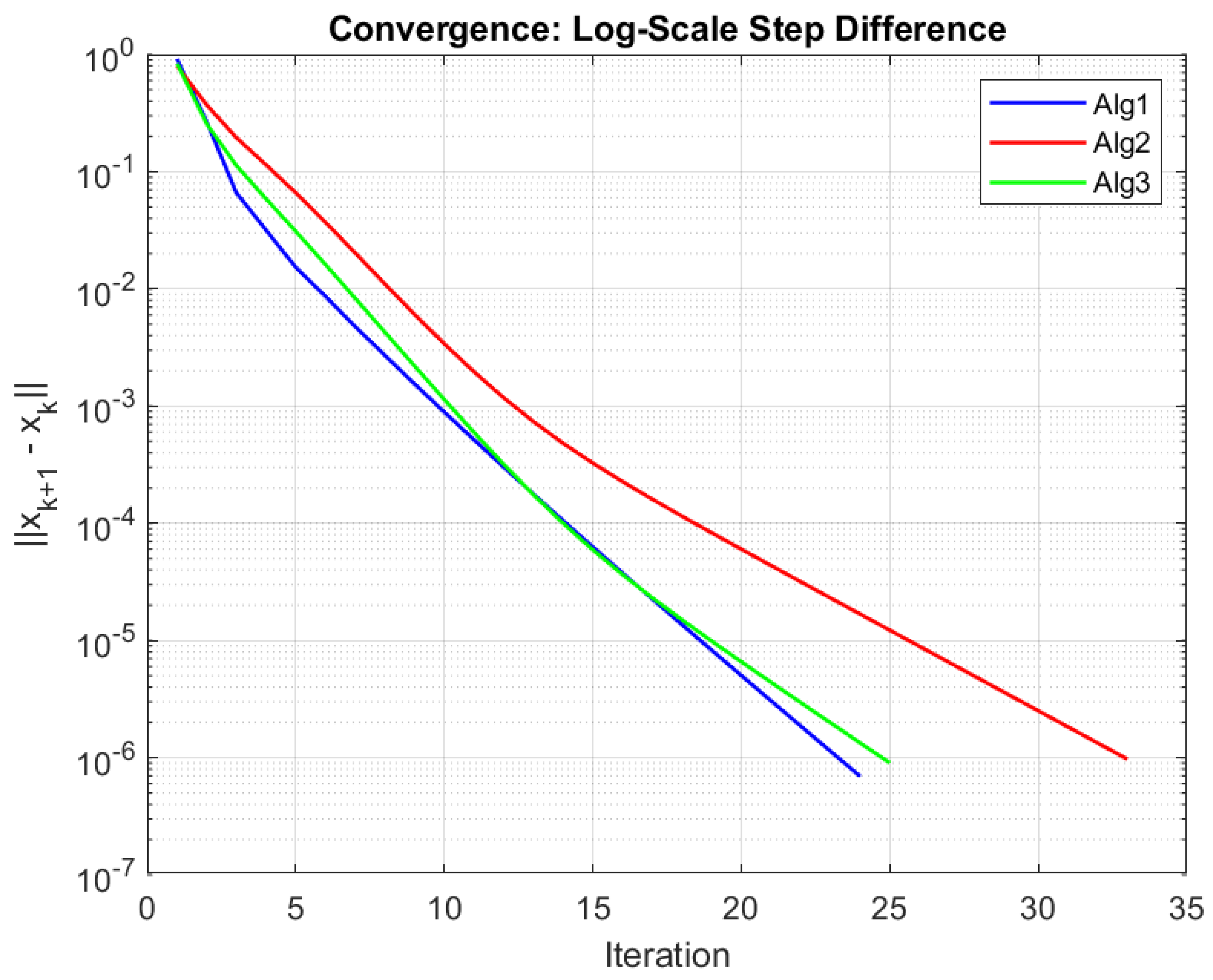
Figure 2 presents a detailed performance profile analysis that concentrates on the number of iterations each algorithm requires. The analysis shows that the proposed algorithm distinctly outperforms the others by requiring the fewest iterations, which indicates that it converges more rapidly when solving QVI problems.

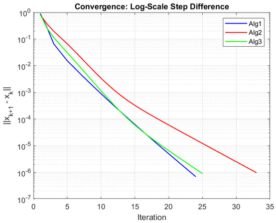
Figure 2. Comparison of the convergence behavior of the forward–backward–forward method (Alg1), the classical gradient projection method (Alg2), and the three-step method (Alg3).

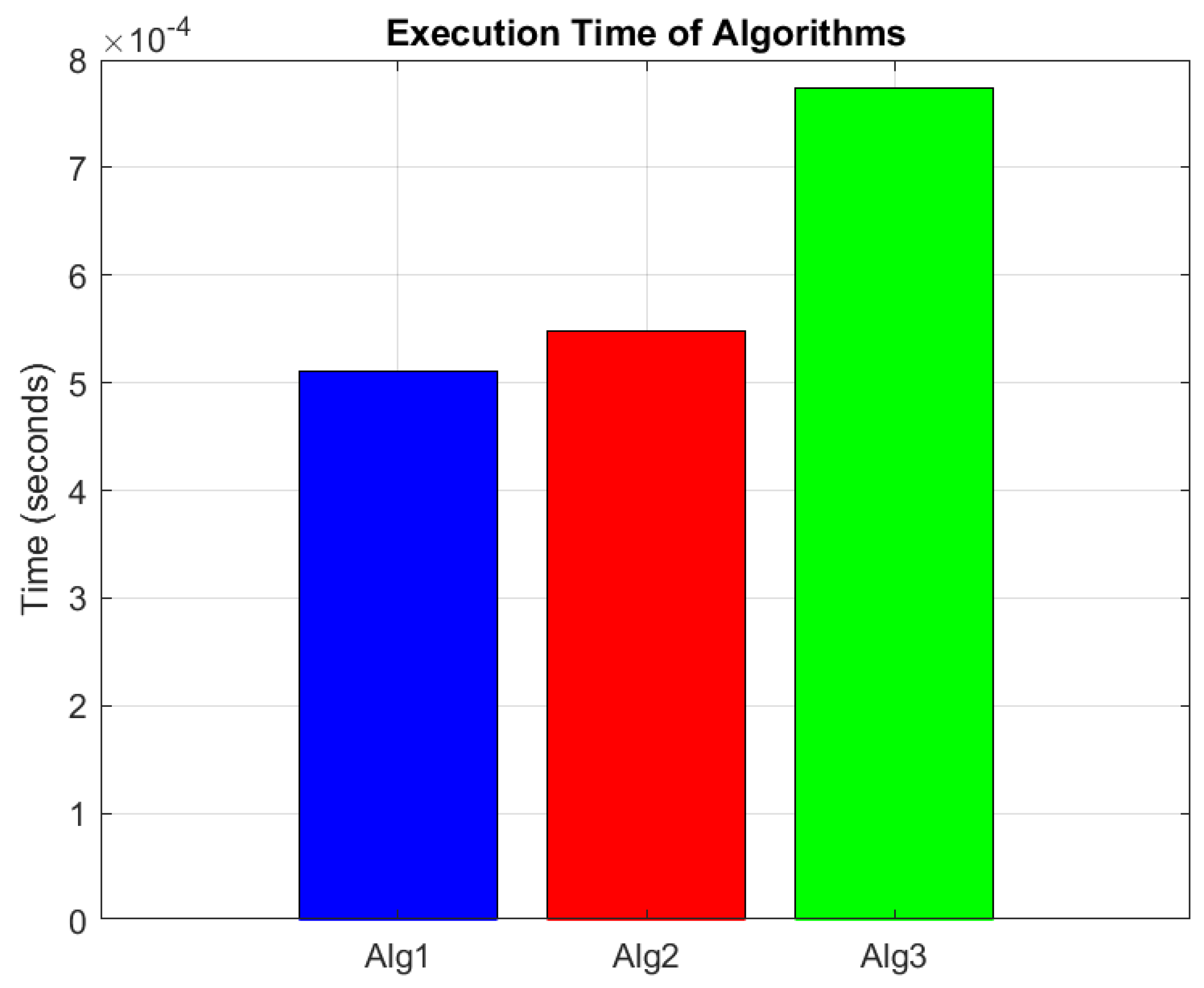
Similarly, we executed the program 10,000 times to record the average execution times for the three algorithms, with the results illustrated in Figure 3. Notably, Alg3 performs three projections in every iteration, which naturally leads to a higher average execution time. These findings collectively confirm that the proposed algorithm is the most efficient choice in terms of both iteration count and execution time for the given function and parameters.

Figure 3. Performance profile based on the average time of execution.

We observe similar outcomes when using alternative values for parameter $\alpha$ that satisfy the conditions of Theorem 2, as well as when employing a different starting point.

6. Conclusions

Our research focused on a quasi-variational inequality defined over a moving set controlled by an operator that is both strongly monotone and Lipschitz continuous. We developed an associated forward–backward–forward dynamical system and conducted a detailed analysis to establish that its trajectories converge asymptotically to a unique solution of the quasi-variational inequality. By explicitly discretizing time in this dynamical system, we derived a forward–backward–forward algorithm. We demonstrated that the sequence of iterates converges to a solution of the quasi-variational inequality and that, under strong monotonicity, this convergence is linear. The numerical comparisons of the proposed algorithm showed that our proposed forward–backward–forward algorithm is efficient and outperforms some related gradient projection-type algorithms in the literature for quasi-variational inequalities. The findings presented in this paper may serve as a catalyst for further research in this field.

References

- Cavazzuti, E.; Pappalardo, M.; Passacantando, M. Nash Equilibria, Variational Inequalities, and Dynamical Systems. J. Optim. Theory Appl. 2002, 114, 491–506. [Google Scholar] [CrossRef]
- Facchinei, F.; Pang, J.S. Finite-Dimensional Variational Inequalities and Complementarity Problems; Springer: New York, NY, USA, 2003. [Google Scholar]
- Kinderlehrer, D.; Stampacchia, G. An Introduction to Variational Inequalities and Their Applications; Classics in Applied Mathematics (Book 31); Society for Industrial and Applied Mathematics: Philadelphia, PA, USA, 1987. [Google Scholar]
- Baiocchi, A.; Capelo, A. Variational and Quasi-Variational Inequalities; Wiley: NewYork, NY, USA, 1984. [Google Scholar]
- Bensoussan, A.; Goursat, M.; Lions, J.L. Contrôle impulsionnel et inéquations quasi-variationnelles stationnaries. Comptes Rendus L’Académie Sci. Paris Ser. A 1973, 276, 1279–1284. [Google Scholar]
- Mosco, U. Implicit variational problems and quasi variational inequalities. In Nonlinear Operators and the Calculus of Variations: Summer School Held in Bruxelles, 8–9 September 1975; Lecture Notes in Mathematics; Springer: Berlin/Heidelberg, Germany, 1976; Volume 543, pp. 83–156. [Google Scholar]
- Bliemer, M.; Bovy, P. Quasi-variational inequality formulation of the multiclass dynamic traffic assignment problem. Transp. Res. Part B Methodol. 2003, 37, 501–519. [Google Scholar] [CrossRef]
- Harker, P.T. Generalized Nash games and quasivariational inequalities. Eur. J. Oper. Res. 1991, 54, 81–94. [Google Scholar] [CrossRef]
- Kocvara, M.; Outrata, J.V. On a class of quasi-variational inequalities. Optim Methods Softw. 1995, 5, 275–295. [Google Scholar] [CrossRef]
- Pang, J.S.; Fukushima, M. Quasi-variational inequalities, generalized Nash equilibria and Multi-leader-follower games. Comput. Manag. Sci. 2005, 1, 21–56. [Google Scholar] [CrossRef]
- Wei, J.Y.; Smeers, Y. Spatial oligopolistic electricity models with Cournot generators and regulated transmission prices. Oper. Res. 1999, 47, 102–112. [Google Scholar]
- Yao, J.C. The generalized quasi-variational inequality problem with applications. J. Math. Anal. Appl. 1991, 158, 139–160. [Google Scholar] [CrossRef]
- Alizadeh, Z.; Jalilzadeh, A. Convergence Analysis of Non-Strongly-Monotone Stochastic Quasi-Variational Inequalities. arXiv 2024, arXiv:2401.03076. [Google Scholar]
- Antipin, A.S.; Jaćimović, M.; Mijajlović, N. Extragradient method for solving quasivariational inequalities. Optimization 2017, 67, 103–112. [Google Scholar] [CrossRef]
- Antipin, A.S.; Mijajlović, N.; Jaćimović, M. A Second-Order Continuous Method for Solving Quasi-Variational Inequalities. Comput. Math. Math. Phys. 2011, 51, 1856–1863. [Google Scholar] [CrossRef]
- Antipin, A.S.; Mijajlović, N.; Jaćimović, M. A Second-Order Iterative Method for Solving Quasi-Variational Inequalities. Comput. Math. Math. Phys. 2013, 53, 258–264. [Google Scholar] [CrossRef]
- Barbagallo, A. Existence results for a class of quasi-variational inequalities and applications to a noncooperative model. Optimization 2024, 1–22. [Google Scholar] [CrossRef]
- Dey, S.; Reich, S. A dynamical system for solving inverse quasi-variational inequalities. Optimization 2024, 73, 1681–1701. [Google Scholar] [CrossRef]
- Facchinei, F.; Kanzow, C.; Karl, S.; Sagratella, S. The semismooth Newton method for the solution of quasi-variational inequalities. Comput. Optim. Appl. 2015, 62, 85–109. [Google Scholar] [CrossRef]
- Facchinei, F.; Kanzow, C.; Sagratella, S. Solving quasi-variational inequalities via their KKT conditions. Math. Program. 2014, 144, 369–412. [Google Scholar] [CrossRef]
- Lara, F.; Marcavillaca, R.T. Bregman proximal point type algorithms for quasiconvex minimization. Optimization 2022, 73, 497–515. [Google Scholar] [CrossRef]
- Mijajlović, N.; Jaćimović, M. Three-step approximation methods from continuous and discrete perspective for quasi-variational inequalities. Comput. Math. Math. Phys. 2024, 64, 605–613. [Google Scholar] [CrossRef]
- Mijajlović, N.; Jaćimović, M. Strong convergence theorems by an extragradient-like approximation methods for quasi-variational inequalities. Optim. Lett. 2023, 17, 901–916. [Google Scholar] [CrossRef]
- Mijajlović, N.; Jaćimović, M.; Noor, M.A. Gradient-type projection methods for quasi-variational inequalities. Optim. Lett. 2019, 13, 1885–1896. [Google Scholar] [CrossRef]
- Mijajlović, N.; Jaćimović, M. Some Continuous Methods for Solving Quasi-Variational Inequalities. Comput. Math. Math. Phys. 2018, 58, 190–195. [Google Scholar] [CrossRef]
- Mijajlović, N.; Jaćimović, M. Proximal methods for solving quasi-variational inequalities. Comput. Math. Math. Phys. 2015, 55, 1981–1985. [Google Scholar] [CrossRef]
- Nguyen, L.V. An existence result for strongly pseudomonotone quasi-variational inequalities. Ric. Mat. 2023, 72, 803–813. [Google Scholar] [CrossRef]
- Nguyen, L.V.; Qin, X. Some Results on Strongly Pseudomonotone Quasi-Variational Inequalities. Set-Valued Var. Anal. 2020, 28, 239–257. [Google Scholar] [CrossRef]
- Noor, M.A.; Noor, K.I. Some new iterative schemes for solving general quasi variational inequalities. Le Matematiche 2024, 79, 327–370. [Google Scholar]
- Shehu, Y. Linear Convergence for Quasi-Variational Inequalities with Inertial Projection-Type Method. Numer. Funct. Anal. Optim. 2021, 42, 1865–1879. [Google Scholar] [CrossRef]
- Shehu, Y.; Gibali, A.; Sagratella, S. Inertial Projection-Type Methods for Solving Quasi-Variational Inequalities in Real Hilbert Spaces. J. Optim. Theory Appl. 2020, 184, 877–894. [Google Scholar] [CrossRef]
- Yao, Y.; Adamu, A.; Shehu, Y. Strongly convergent inertial forward-backward-forward algorithm without on-line rule for variational inequalities. Acta Math. Sci. 2024, 44, 551–566. [Google Scholar] [CrossRef]
- Yao, Y.; Jolaoso, L.O.; Shehu, Y. C-FISTA type projection algorithm for quasi-variational inequalities. Numer. Algor. 2025, 98, 1781–1798. [Google Scholar] [CrossRef]
- Banert, S.; Bot, R.I. A forward-backward-forward differential equation and its asymptotic properties. J. Convex Anal. 2018, 25, 371–388. [Google Scholar]
- Tseng, P. A modified forward-backward splitting method for maximal monotone mappings. SIAM J. Control Optim. 2000, 38, 431–446. [Google Scholar] [CrossRef]
- Wang, K.; Wang, Y.; Shehu, Y.; Jiang, B. Double inertial Forward–Backward–Forward method with adaptive step-size for variational inequalities with quasi-monotonicity. Commun. Nonlinear Sci. Numer. Simul. 2024, 132, 107924. [Google Scholar] [CrossRef]
- Yin, T.C.; Hussain, N. A Forward-Backward-Forward Algorithm for Solving Quasimonotone Variational Inequalities. J. Funct. Spaces 2022, 2022, 7117244. [Google Scholar] [CrossRef]
- Bot, R.I.; Csetnek, E.R.; Vuong, P.T. The Forward-Backward-Forward Method from continuous and discrete perspective for pseudo-monotone variational inequalities in Hilbert spaces. Eur. J. Oper. Res. 2020, 287, 49–60. [Google Scholar] [CrossRef]
- Bot, R.I.; Mertikopoulos, P.; Staudigl, M.; Vuong, P.T. Minibatch forward- backward-forward methods for solving stochastic variational inequalities. Stoch. Syst. 2021, 11, 112–139. [Google Scholar] [CrossRef]
- Izuchukwu, C.; Shehu, Y.; Yao, J.C. New inertial forward-backward type for variational inequalities with Quasi-monotonicity. J. Glob. Optim. 2022, 84, 441–464. [Google Scholar] [CrossRef]
- Attouch, H.; Czarnecki, M.-O.; Peypouquet, J. Coupling Forward-Backward with Penalty Schemes and Parallel Splitting for Constrained Variational Inequalities. SIAM J. Optim. 2011, 21, 1251–1274. [Google Scholar] [CrossRef]
- Ryazantseva, I.P. First-order methods for certain quasi-variational inequalities in a Hilbert space. Comput. Math. Math. Phys. 2007, 47, 183–190. [Google Scholar] [CrossRef]
- Vasil’ev, F.P. Optimization Methods; Faktorial Press: Moscow, Russia, 2002. [Google Scholar]
- Nesterov, Y.; Scrimali, L. Solving strongly monotone variational and quasi-variational inequalities. Discret. Contin. Dyn. Syst. 2011, 31, 1383–1396. [Google Scholar] [CrossRef]
- Noor, M.A.; Oettli, W. On general nonlinear complementarity problems and quasi-equilibria. Le Matematiche 1994, 49, 313–331. [Google Scholar]
Disclaimer/Publisher’s Note: The statements, opinions and data contained in all publications are solely those of the individual author(s) and contributor(s) and not of MDPI and/or the editor(s). MDPI and/or the editor(s) disclaim responsibility for any injury to people or property resulting from any ideas, methods, instructions or products referred to in the content. |
© 2025 by the authors. Licensee MDPI, Basel, Switzerland. This article is an open access article distributed under the terms and conditions of the Creative Commons Attribution (CC BY) license (https://creativecommons.org/licenses/by/4.0/).