A Stochastic Model for Traffic Incidents and Free Flow Recovery in Road Networks

Abstract

This study addresses the disruptive impact of incidents on road networks, which often lead to traffic congestion. If not promptly managed, congestion can propagate and intensify over time, significantly delaying the recovery of free-flow conditions. We propose an enhanced model based on an exponential decay of the time required for free flow recovery between incident occurrences. Our approach integrates a shot noise process, assuming that incidents follow a non-homogeneous Poisson process. The increases in recovery time following incidents are modeled using exponential and gamma distributions. We derive key performance metrics, providing insights into congestion risk and the unlocking phenomenon, including the probability of the first passage time for our process to exceed a predefined congestion threshold. This probability is analyzed using two methods: (1) an exact simulation approach and (2) an analytical approximation technique. Utilizing the analytical approximation, we estimate critical extreme quantities, such as the minimum incident clearance rate, the minimum intensity of recovery time increases, and the maximum intensity of incident occurrences required to avoid exceeding a specified congestion threshold with a given probability. These findings offer valuable tools for managing and mitigating congestion risks in road networks.

1. Introduction

The traffic flow of road networks is subject to a delicate balance between travel demand and network capacity. However, this equilibrium can be disturbed by various incidents such as accidents, road work, breakdowns, etc. These incidents lead to traffic congestion, which degrades the capacity of networks and amplifies disturbances. Disruptions can even appear when incidents are not treated and solved in time. In this work, we focus on modeling the occurrence and duration of such incidents, specifically the time needed for free flow recovery. Our research is based on an existing stochastic risk model for incident occurrences and duration in road networks [1], which assumes a linear decay in the time between consecutive incident occurrences. In this work, we propose a reformulation of the model with an exponential decay of the time between consecutive incident occurrences. This modification allows us to better capture the temporal dynamics of incident occurrences and their impact on traffic flow.

One of our aims is to capture the dynamics of the system, for which we make certain assumptions. We consider an initial traffic state before incident occurrences. Then, we assume that the increases in the time needed for free flow recovery after incident occurrences follow probability distributions such as gamma and exponential distributions. Lastly, we model the incident occurrences using a non-homogeneous Poisson process. We then develop our model and derive some interesting performance characteristics. These derivations are performed using exact methods whenever possible, and approximate methods are employed when exact solutions are not feasible. The derived characteristics include the expected and variance values of the time needed for the free flow recovery process, the expected value of the first time when the process exceeds a given congestion threshold, and the probability for the process to exceed a specified congestion threshold for the first time. To compute the latter probability, we employ two distinct methods: (1) an exact simulation method and (2) an analytic approximation method. The latter method relies on computing the expected value of the first time when the process exceeds a given congestion threshold. The derivation of these performance characteristics allows us to gain valuable insights into the behavior of the free flow recovery process and its associated congestion risks. These results contribute to a deeper understanding of the dynamics of road networks and aid in the development of effective strategies to manage and mitigate congestion.

We illustrate our model and results with some numerical approximations for several extreme quantities, including the following: the approximate minimum incident clearance rate, the approximate maximum intensity of the incident occurrence process, and the approximate maximum average value of the increment in the time needed for free flow recovery following incident occurrences, all of which are requisite to limit congestion level with respect to a specified probability. We also illustrate our findings with examples, figures, and thorough interpretations and discussions. These results highlight the applicability and effectiveness of capturing incident-induced congestion dynamics in road networks.

The structure of this paper is organized as follows. Section 2 presents existing works in the literature relevant to our contribution. Section 3 introduces our new model, where we assume an exponential decay for the time needed for the free flow recovery process in road networks. We provide a comprehensive performance analysis of the time needed for free flow recovery, including an examination of the probability of the first passage time for our process to exceed a given congestion threshold. In Section 4, we present the results of numerical simulations conducted for our proposed model. Section 5 focuses on the practical applications of our model under two specific cases and various traffic conditions. Finally, in Section 6, we summarize our findings, draw meaningful conclusions from the study, and outline potential avenues for future research.

2. Existing Works

The existing literature includes numerous studies on modeling traffic incidents, non-recurrent congestion, and incident duration and frequency. These studies have advanced various techniques and methods in the field. Notably, three prominent research areas have garnered significant attention:

Incident duration and frequency prediction models: Significant research focuses on models that predict traffic incident duration and frequency to improve traffic management and control. These models provide insights into incident dynamics and help assess their impact on road networks. Previous studies employed various distributions to fit incident duration based on observed datasets in road networks, such as the log-normal distribution [2]. The authors of [3] introduced a parametric log-logistic accelerated failure time model for predicting incident duration. In [4], a mixture risk competing approach to predict the duration of different types of incidents was employed. In [5], a Weibull accelerated failure time model to fit the clearance accident duration was used. The authors of [6] proposed a non-parametric regression model to estimate incident duration. Moreover, in [7], tree-structured quantile regression was incorporated to model incident duration. Bayesian networks were used in [8] to fit the detected incident duration. Machine learning techniques were also employed for incident duration prediction, as demonstrated in [9]. The authors of [10] applied artificial neural networks to model the sequential prediction of incident duration. Additionally, in [11], a comparative analysis of existing methods was conducted for predicting incident duration in road networks.

Stochastic approach modeling the impact of incident occurrences on road traffic flow: Stochastic modeling approaches have been widely used to understand the complex behavior of traffic flow in the presence of incidents. Incidents, being stochastic events themselves, have the potential to disrupt traffic flow within road networks. In [12], the authors addressed this by modeling the occurrence process and clearance time of incidents using an $M/M/c$ queuing system. This approach provided insights into the queuing behavior of incidents and their impact on traffic flow. To capture the resulting traffic congestion from incidents, the authors of [13] introduced a discrete-time non-linear stochastic model. The latter effectively captured the dynamic effects of incidents on traffic flow, enabling a comprehensive analysis of congestion patterns. In response to incidents, a stochastic optimal control framework to manage real-time control of highway ramps was proposed in [14]. The approach aimed to optimize traffic operations by considering the stochastic nature of incidents and their impact on the ramp control strategies.

Traffic safety and risk assessment: Another crucial research area related to our work is assessing risks associated with road traffic incidents. Studies aim to quantify risks and develop methods for evaluating the safety implications of incidents. These assessments help to create proactive strategies and policies for incident management and road safety improvement. Extensive research has explored traffic safety risks, including incident and congestion risks, using various methodologies. There are studies that focus on incident risk as in [15] where the authors employed a K-means clustering analysis method to create clusters representing different traffic flow states. They investigated the correlation between accident risk and these traffic states by constructing conditional logistic regression models. In another study [16], the focus was on predicting real-time accident precursor risk across various types of freeway sections. There are other studies that examine congestion risk, such as the statistical analysis implemented in [17] to measure both recurrent and non-recurrent traffic congestion across different freeway sections. With another approach, a dynamic Bayesian graph convolution network was developed to model the propagation of both recurrent and non-recurrent traffic congestion [18].

Our contributions: Our modeling approach differs from the existing ones in the literature. We incorporated here a new class of continuous temporal processes, based on piece-wise deterministic Markov processes (PDMPs). Specifically, in our modeling, we capture the dynamics of the evolution of the time needed for free flow recovery after incident occurrences. Our first contribution consists in the derivation of congestion risk, which also differs from the literature. Our congestion risk is calculated as the probability that the time needed for free flow recovery exceeds a certain threshold. We notice that some existing models are limited to estimating incident duration, whereas our model combines the effect on time due to incident occurrences and free flow recovery after cleared incidents. The model proposed in this article presents a reformulation of the existing model in [1]. Our model assumes an exponential decay of the time needed for free flow recovery, instead of a linear decay as assumed in [1]. From this extension, we give some explicit formulas and analytic approximations for certain indicators and measures of interest, interpreted in terms of traffic resulting from incidents.

3. The Model

In this section, we present our stochastic model for the evolution of the time needed for free flow recovery following incident occurrences in a road network. The key feature of our model is the assumption of an exponential decay in contrast to the linear decay considered in the model presented in [1]. The introduction of an exponential decay in our model allows for its applicability across all values of the time needed for free flow recovery. Unlike the existing model [1], which necessitates re-initialization when the required time for free flow recovery approaches zero, our extended model can handle all values of the time needed for free flow recovery without any constraints. Assuming that the time needed for free flow recovery is exponential, this is like assuming that the non-recurrent congestion clearance speed is linear and depends on the incident clearance rate. We note that this rate can be given by its average over the free flow recovery time, which permits us to calibrate this rate in practice.

In our model, we maintain two important assumptions, traffic homogeneity and stability, similar to the case of a linear decay in the required time for free flow recovery [1]. The inclusion of the first assumption (traffic homogeneity) is critical, as it enables the modeling of the traffic state using a stochastic process. This assumption assumes that traffic conditions remain consistent and do not vary significantly across the road network or the specific part of the network under consideration. The second assumption (stability) is necessary to ensure the reliability of all the parameters that govern the model throughout the specified time period. This assumption guarantees that the model remains consistent and applicable over the entire duration of interest, providing meaningful and accurate results. It ensures that the underlying factors influencing the time needed for free flow recovery remain stable and do not undergo significant changes that could affect the validity of the model.

In our modeling approach, we focus exclusively on primary incidents occurring on a specific road section or part of a road network. Secondary incidents, the spread of incidents, and correlations among flows on adjacent roads are not considered. This simplification allows us to focus on analyzing the direct impacts of primary incidents on traffic flow.

The model we present here is based on piece-wise deterministic Markov processes (PDMPs) elaborated by Davis [19], and also used to model food risk in [20]. Our main variable here is the stochastic process X, where $X(s)$ denotes the time needed for free flow recovery in a road network, at time step s, after incident occurrences. We characterize the time needed for free flow recovery between two consecutive incident occurrences with an exponential decay by assuming a linear stochastic differential equation, which is given as follows:

$$\dot{X}(s)=-V(X(s),c)=-cX(s),$$

(1)

where

• $X(s)$ is the time needed for free flow recovery, at time s.
• $V(X(s),c)$ is a function modeling the non-recurrent congestion speed clearance assumed to be linear.
• c is a parameter modeling the incident clearance rate. This rate c can be constant or stochastic.

From Equation (1), ${\left\{X(t)\right\}}_{t\ge 0}$ is given as follows (see, for example, [20]):

$$X(t)=X(0)+\sum _{i=1}^{N(t)}{W}_i-\sum _{i=1}^{N(t)+1}{\int }_{T_{i-1}}^{min(T_i,t)}V(X(s),c)ds,$$

(2)

where

• $W_i$ are the increases in the time needed for flow recovery after incident occurrences, for $i\ge 1$.
• $T_i$ with $T_0=0$ represent the incident occurrence times, for $i\ge 1$.
• ${\displaystyle N(t)=\sum _{i=1}^{\infty }{\mathbf{1}}_{\{T_i\le t\}}}$ gives the counting number of incident occurrences before time t. The incident occurrence process is denoted by ${\left\{N(t)\right\}}_{t\ge 0}$.

Then, by rearranging (2), we obtain a shot noise process as follows [21]:

$$X(t)=X(0)e^{-ct}+\sum _{i=1}^{N(t)}{W}_i{e}^{-c(t-T_i)}$$

(3)

A discrete-time expression of (3) is an auto-regressive process (see, for example, [20]):

$${\displaystyle X(T_i)=X(T_{i-1})e^{-c\Delta T_i}+W_i\mathrm{if}i\ge 1,\mathrm{with}X(T_0)=X(0).}$$

(4)

We denote $x_0:=X(0)$ as the initial state of the process ${\left\{X(t)\right\}}_{t\ge 0}$.

For the model we propose here, we assume the following:

• The random variables ${(W_i)}_{i\in {\mathbb{N}}^{\ast }}$ are assumed to be mutually independent and identically distributed. We denote by $F_W(w):=P(W_i\le w)$ the cumulative distribution probability of ${(W_i)}_{i\in {\mathbb{N}}^{\ast }}$.
• The random variables ${(T_i)}_{i\in {\mathbb{N}}^{\ast }}$ with $T_0=0$ are assumed to be independent.
• The random variables ${(\Delta T_i:=T_i-T_{i-1})}_{i\in {\mathbb{N}}^{\ast }}$ (which represent here the incident inter-occurrence times) are assumed to be mutually independent and identically distributed with a cumulative distribution probability $G(s):=P(\Delta T_i\le s)$.
• The two random variables ${(W_i)}_{i\in {\mathbb{N}}^{\ast }}$ and the process ${\left\{N(t)\right\}}_{t\ge 0}$ are independent.

Let us fix the following additional notation:

• ${\displaystyle Z(t):=\sum _{i=1}^{N(t)}{W}_i}$ denotes the cumulative increase in the time needed for free flow recovery after incident occurrences.
• b is a constant denoting the threshold on the time needed for free flow recovery, i.e., the congestion threshold.

We are interested in this paper in the derivation of some performance characteristics of the process ${\left\{X(t)\right\}}_{t\ge 0}$ having interpretations in terms of traffic flow recovery and traffic incidents in road networks. These performance characteristics are defined as follows:

• The expected values $m_X(t)$ and $m_X$ have finite and infinite time horizons, respectively, and the variance values ${\sigma }_X^2(t)$ and ${\sigma }_X^2$ have finite and infinite time horizons for the process ${\left\{X(t)\right\}}_{t\ge 0}$. The two quantiles represent the expectations of the time needed for free flow recovery process and their variations for the finite and infinite time horizons, respectively.
• Let $\tau$ denote the time needed for the free flow recovery to exceed a given congestion threshold b, defined as follows:

  $$\tau :=inf\{s\ge 0,X(s)>b\mid X(0)=x_0\}.$$

  (5)
  We are interested in approximating the expected value ${\displaystyle {\mathbb{E}}_{x_0}(\tau )}$.
• The cumulative distribution probability $F_{\tau }$ of $\tau$ is as follows:

  $$\begin{array}{c}\hfill F_{\tau }(t):=P\left(\tau \le t\right)=P\left(inf\{s\ge 0,X(s)>b\mid X(0)=x_0\}\le t\right).\end{array}$$

  (6)
  We can link this probability distribution to ${sup}_{0\le s\le t}X(s)$ as follows:

  $${\displaystyle F_{\tau }(t)=P\left(\underset{0\le s\le t}{sup}X(s)>b\mid X(0)=x_0\right).}$$

  (7)

Figure 1 illustrates the evolution of the time needed for free flow recovery, with a linear non-recurrent congestion speed clearance.

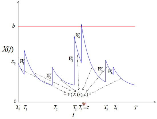
Figure 1. Illustration of process ${\left\{X(t)\right\}}_{t\ge 0}$ (blue curve), with presentations of first passage time $\tau$ (red arrow) and congestion threshold b (red line).

3.1. Performance Characteristics of Time Needed for Free Flow Recovery Process ${\left\{X(t)\right\}}_{t\ge 0}$

We derive in this subsection some performance characteristics defined above for the process ${\left\{X(t)\right\}}_{t\ge 0}$ as given in (3). Specifically, these performance characteristics are determined for the two specific cases where the incident occurrence process ${\left\{N(t)\right\}}_{t\ge 0}$ follows a non-homogeneous Poisson distribution with intensity $\lambda (t)>0,\forall t\ge 0$, and the increases in the time needed for free flow recovery after incident occurrences ${(W_i)}_{i\in {\mathbb{N}}^{\ast }}$ are independent and identically distributed, with exponential distribution of intensity $\mu$ and gamma distribution with parameters $\alpha$ and $\beta$.

3.1.1. The Probability Distribution of the Time Needed for Free Flow Recovery Process ${\left\{X(t)\right\}}_{t\ge 0}$

We give as follows the cumulative distribution function (cdf) and the probability density function (pdf) denoted, respectively, by $F_X$ and $f_X$ for the time needed for free flow recovery process ${\left\{X(t)\right\}}_{t\ge 0}$:

$$\begin{array}{cc}\hfill {\displaystyle F_X(x,t)}& {\displaystyle =P(X(t)\le x)=P(x_0{e}^{-ct}+\sum _{i=1}^{N(t)}{W}_i{e}^{-c(t-T_i)}\le x)}\hfill \\ \hfill & {\displaystyle =\sum _{n=0}^{\infty }P\left(\sum _{i=1}^{N(t)}{W}_i{e}^{-c(t-T_i)}\le x-x_0{e}^{-ct}\mid N(t)=n\right)P(N(t)=n)}\hfill \\ \hfill {\displaystyle }& {\displaystyle =\sum _{n=0}^{\infty }{H}_{W,T}^{\ast n}(x-x_0{e}^{-ct})P(N(t)=n),}\hfill \end{array}$$

(8)

and

$$\begin{array}{cc}\hfill {\displaystyle f_X(x,t)}& {\displaystyle =\frac{\partial F_X(x,t)}{\partial x}=\sum _{n=0}^{\infty }{h}_{W,T}^{\ast n}(x-x_0{e}^{-ct})P(N(t)=n).}\hfill \end{array}$$

(9)

For the calculated $f_X$ and $F_X$, we use and assume the following:

• $f_W$ and $F_W$ denote, respectively, the probability density and the cumulative distribution functions of the random variables ${(W_i)}_{i\in {\mathbb{N}}^{\ast }}$, which are assumed to be independent and identically distributed.
• ${\left\{N(t)\right\}}_{t\ge 0}$ is a non-homogeneous Poisson process; hence, $P(N(t)=n)={\displaystyle \frac{{(\Lambda (t))}^n}{n!}}{e}^{-\Lambda (t)}$, with $\Lambda (t)={\int }_0^t\lambda (s)ds$.
• The conditional probability density function of the random variables ${(T_i)}_{i\in {\mathbb{N}}^{\ast }}$ is $k_T(s)={\displaystyle \frac{\lambda (s)}{\Lambda (t)}}$.
• The joint cumulative distribution function ${\displaystyle H_{W,T}^{\ast n}}$ (for $n\ge 2$) is the n-fold convolution of the joint cumulative distribution function ${\displaystyle H_{W,T}^{\ast 1}=H_{W,T}}$. Then, ${\displaystyle H_{W,T}}$ is as follows:

  $$\begin{array}{cc}\hfill H_{W,T}(x-x_0{e}^{-ct})& ={\int }_0^{t}P\left(W_i{e}^{-c(t-T_i)}\le x-x_0{e}^{-ct}\mid T_i=s\right)k_T(s)ds\hfill \\ \hfill & ={\int }_0^{t}P(W_i\le \left((x{e}^{ct}-x_0)e^{-cs}\right)k_T(s)ds\hfill \\ \hfill & ={\displaystyle \frac{t}{\Lambda (t)}}{\int }_0^1{F}_W\left((x{e}^{ct}-x_0)e^{-cty}\right)\lambda (yt)dy.\hfill \end{array}$$

  (10)
  We obtain the last Formula (10) by considering a change of variable defined as follows:

  $$y={\displaystyle \frac{s}{t}},\mathrm{which}\mathrm{implies}dy={\displaystyle \frac{1}{t}}ds.$$
  Under this transformation:
  • When $s=0$, $y=0$;
  • When $s=t$, $y=1$.
• The joint probability density function ${\displaystyle h_{W,T}^{\ast n}}$ (for $n\ge 2$) is the n-fold convolution of the joint probability density function ${\displaystyle h_{W,T}^{\ast 1}=h_{W,T}}$. Then, ${\displaystyle h_{W,T}}$ is as follows:

  $$\begin{array}{cc}\hfill h_{W,T}\left(x-x_0{e}^{-ct}\right)& ={\displaystyle \frac{\partial H_{W,T}(x-x_0{e}^{-ct})}{\partial x}}={\displaystyle \frac{t}{\Lambda (t)}}{\int }_0^1{f}_W\left((x{e}^{ct}-x_0)e^{-cty}\right)\lambda (yt)dy.\hfill \end{array}$$

  (11)

For detailed derivations of the cumulative distribution function (cdf) and the probability density function (pdf) $F_X$ (given in (8)) and $f_X$ (given in (9)) for the time needed for free flow recovery process ${\left\{X(t)\right\}}_{t\ge 0}$ in our two specific cases where the incident occurrences process ${\left\{N(t)\right\}}_{t\ge 0}$ follows a homogeneous Poisson with intensity $\lambda$, (i.e., $\lambda (t)=\lambda ,\forall t\ge 0$), and the increases in the time needed for free flow recovery after incident occurrences ${(W_i)}_{i\in {\mathbb{N}}^{\ast }}$ are independent and identically distributed, with an exponential distribution of intensity $\mu$ and a gamma distribution with parameters $\alpha$ and $\beta$, refer to Appendix A.

3.1.2. The Expected and Variance Values of the Time Needed for the Free Flow Recovery Process

We give in this subsection the expected and the variance values of the time needed for free flow recovery process ${\left\{X(t)\right\}}_{t\ge 0}$:

$$\begin{array}{cc}\hfill {\displaystyle m_X(t)}& {\displaystyle =\mathbb{E}(X(t))=\mathbb{E}\left(x_0{e}^{-ct}+\sum _{i=1}^{N(t)}{W}_i{e}^{-c(t-T_i)}\right)=x_0{e}^{-ct}+\mathbb{E}\left(\sum _{i=1}^{N(t)}{W}_i{e}^{-c(t-T_i)}\right),}\hfill \end{array}$$

and

$$\begin{array}{cc}\hfill {\sigma }_X^2(t)& {\displaystyle =\mathbb{V}(X(t))=\mathbb{V}\left(x_0{e}^{-ct}+\sum _{i=1}^{N(t)}{W}_i{e}^{-c(t-T_i)}\right)=\mathbb{V}\left(\sum _{i=1}^{N(t)}{W}_i{e}^{-c(t-T_i)}\right).}\hfill \end{array}$$

In the following, we use items 1, 2, and 3 from Section 3.1.1. According to [22], the moment generating function (mgf) of the process ${\displaystyle {\left\{Y(t)\right\}}_{t\ge 0}}$ defined by ${\displaystyle Y(t)=\sum _{i=1}^{N(t)}{W}_i{e}^{-c(t-T_i)}}$ is written as follows:

$$\begin{array}{c}\hfill {\displaystyle \mathbb{E}\left(e^{uY(t)}\right)=e^{-\Lambda (t)}\sum _{n=0}^{\infty }\frac{{(M(u,t)\Lambda (t))}^n}{n!}=e^{\Lambda (t)(M(u,t)-1)},}\end{array}$$

where ${\displaystyle M(u,t)={\int }_0^t{k}_T(s)\psi (u{e}^{-c(t-s)})ds}$, and ${\displaystyle \psi (u{e}^{-c(t-s)})={\int }_{-\infty }^{+\infty }{e}^{uw{e}^{-c(t-s)}}{f}_W(w)dw}$. Finally, the expected and the variance values for the time needed for the free flow recovery process are as follows:

$$\begin{array}{cc}\hfill {\displaystyle m_X(t)}& =x_0{e}^{-ct}+{\left|{\displaystyle \frac{{\displaystyle \partial \mathbb{E}\left(e^{uY(t)}\right)}}{\partial u}}\right|}_{u=0}=x_0{e}^{-ct}+\mathbb{E}(W_i){\int }_0^t\lambda (s)e^{-c(t-s)}ds,\hfill \end{array}$$

and

$$\begin{array}{cc}\hfill {\displaystyle {\sigma }_X^2(t)}& ={\left|{\displaystyle \frac{{\displaystyle {\partial }^2\mathbb{E}\left(e^{uY(t)}\right)}}{{\partial }^{2}u}}\right|}_{u=0}-{\left|{\displaystyle \frac{{\displaystyle \partial \mathbb{E}\left(e^{uY(t)}\right)}}{\partial u}}\right|}_{u=0}^2=\mathbb{E}(W_i^2){\int }_0^t\lambda (s)e^{-2c(t-s)}ds.\hfill \end{array}$$

Refer to Appendix B for detailed derivations of the expected and variance values of the time needed for the free flow recovery process in the two particular cases considered in Section 3.1.1.

3.1.3. The Probability Distribution of the First Passage Time for Process ${\left\{X(t)\right\}}_{t\ge 0}$ to Exceed a Given Congestion Threshold

In this part, we propose a method that approximates the probability distribution of the first passage time for our process ${\left\{X(t)\right\}}_{t\ge 0}$ to exceed a given congestion threshold, defined in (6) and (7). According to [23], this method is based on a martingale families technique. Let us first give some definitions.

Definition 1. 

We define several functions and quantities as follows (see [23]):

• Let ${\displaystyle K:=sup\{u\ge 0:\mathbb{E}{e}^{uZ(1)}<\infty \}}$, where $\mathbb{E}{e}^{uZ(1)}=e^{\lambda (m_W(u)-1)}$ is the moment generating function of $Z(t)$. Here, $Z(t)$ represents the cumulative increase in the time needed for free flow recovery after incident occurrences evaluated at $t=1$, and $m_W(u)$ is the moment generating function of the random variables ${(W_i)}_{i\in {\mathbb{N}}^{\ast }}$ of the increases in the time needed for free flow recovery after incident occurrences.
• For $u<K$, we let $\varphi (u):=log(\mathbb{E}{e}^{uZ(1)})$, and ${\displaystyle g(u)=\frac{1}{c}{\int }_0^u{y}^{-1}\varphi (y)dy}$.
• Let ${\Delta }_b(c):=X(\tau )-b$ generally be with an unknown distribution and assumed to be independent of τ. We can see that $X(\tau )$ corresponds to the value of the process ${\left\{X(t)\right\}}_{t\ge 0}$ at $t=\tau$, which is also influenced by the rate c; see (3). Then, under these conditions ($b\to \infty$, $c\to 0$), we have ${\Delta }_b(c)\to {\Delta }_b(0)$ as $c\to 0$ and ${\Delta }_b(0)\to R_{\infty }$ as $b\to \infty$.

Proposition 1. 

The probability distribution of the first passage time for our process ${\left\{X(t)\right\}}_{t\ge 0}$ to exceed a given congestion threshold is approximated as follows [23]:

$$F_{\tau }(t):=P\left(\tau \le t\right)\approx H_{\tau }(t):=1-exp\left(-{\displaystyle \frac{t}{{\mathbb{E}}_{x_0}(\tau )}}\right),$$

(12)

where ${\displaystyle {\mathbb{E}}_{x_0}(\tau )}$ is the expected value of the first passage time for our process ${\left\{X(t)\right\}}_{t\ge 0}$ to exceed a given congestion threshold ${\displaystyle {\mathbb{E}}_{x_0}(\tau )}$, which is given as follows:

$${\displaystyle {\mathbb{E}}_{x_0}(\tau )=\frac{1}{c}{\int }_0^K\left({\mathbb{E}}_{x_0}(e^{u{\Delta }_b(c)})-e^{u(x_0-b)}\right)u^{-1}{e}^{ub-g(u)}du.}$$

(13)

We can also write ${\displaystyle {\mathbb{E}}_{x_0}(\tau )}$ as follows:

$${\displaystyle {\mathbb{E}}_{x_0}(\tau )=\frac{1}{c}{\int }_0^K\left({\mathbb{E}}_{x_0}(e^{u{R}_{\infty }})-e^{u(x_0-b)}\right)u^{-1}{e}^{ub-g(u)}du,}$$

(14)

where Definition 1 covers all necessary parameters and functions used in this proposition.

Proof. 

We refer the reader to Section 3 of  [23] (and the references cited therein), which can be viewed as a technical proof of Proposition 1.    □

Remark 1. 

Let us consider the case where the incident occurrences process is Poisson with intensity λ, and the increases in the time needed for free flow recovery after incident occurrences ${(W_i)}_{i\in {\mathbb{N}}^{\ast }}$ are gamma distributed with two parameters α and β. In this specific case, we denote the function g by ${\displaystyle g^{(P,G)}}$, the expected value of the first passage time for our process ${\left\{X(t)\right\}}_{t\ge 0}$ to exceed a given congestion threshold by ${\mathbb{E}}_{x_0}^{(P,G)}(\tau )$, and the exponential approximation probability of the first passage time for our process ${\left\{X(t)\right\}}_{t\ge 0}$ to exceed a given congestion threshold by $H_{\tau }^{(P,G)}(t)$. Then, we have the following.

• The function ${\displaystyle g^{(P,G)}}$ is given as follows:

  $${\displaystyle g^{(P,G)}(u):=\frac{\lambda }{c}{\int }_0^u\frac{{(1-\beta y)}^{-\alpha }-1}{y}dy=\frac{\lambda }{c}\beta \alpha u{}_{3}F_2(1,1,\alpha +1;2,2;\beta u),u<\frac{1}{\beta },}$$

  (15)

  where ${\displaystyle {}_{3}F_2(1,1,1+\alpha ;2,2;\beta u)=\sum _{n=0}^{\infty }\frac{{(1)}_n{(1)}_n{(1+\alpha )}_n}{{(2)}_n{(2)}_n}\frac{{(\beta u)}^n}{n!}}$ is the specific function of the generalized hyper-geometric function, and ${(.)}_n={\displaystyle \frac{\Gamma (.+n)}{\Gamma (.)}}$, where ${(.)}_n$ is the Pochhammer symbol, and $\Gamma (.)$ is the gamma function.
• The expected value of the first passage time for our process ${\left\{X(t)\right\}}_{t\ge 0}$ to exceed a given congestion threshold ${\mathbb{E}}_{x_0}^{(P,G)}(\tau )$ is given as follows:

  $$\begin{array}{cc}\hfill {\displaystyle }& \hfill {\mathbb{E}}_{x_0}^{(P,G)}(\tau )={\displaystyle \frac{1}{c}}{\int }_0^K\left(M_{\alpha ,\beta }(u)-e^{u(x_0-b)}\right)u^{-1}exp\left(ub-{\displaystyle \frac{\lambda }{c}}\beta \alpha u{}_{3}F_2(1,1,\alpha +1;2,2;\beta u)\right)\\ & \hfill du,K={\displaystyle \frac{1}{\beta }},u<K,\end{array}$$

  (16)

  where ${\displaystyle {\mathbb{E}}_{x_0}(e^{u{R}_{\infty }}):=\sum _{n=0}^{\infty }\frac{u^n}{n!}\mathbb{E}(R_{\infty }^n)=\sum _{n=0}^{\infty }\frac{u^n}{n!}\frac{\mathbb{E}(W_i^{n+1})}{(n+1)\mathbb{E}(W_i)}}$.
  Specifically for this case, we have

  $${\displaystyle {\mathbb{E}}_{x_0}(e^{u{R}_{\infty }})=M_{\alpha ,\beta }(u)=\sum _{n=0}^{\infty }\frac{{(\beta u)}^n}{(n+1)!}{(\alpha +1)}_n=\frac{{(1-\beta u)}^{-\alpha }-1}{\alpha \beta u}.}$$
  By putting $\beta u=v$, and $\beta du=dv$, we obtain

  $$\begin{array}{cc}\hfill {\displaystyle }& {\mathbb{E}}_{x_0}^{(P,G)}(\tau )={\displaystyle \frac{1}{c}}{\int }_0^K\left({\displaystyle \frac{{(1-v)}^{-\alpha }-1}{\alpha v}}-e^{{\displaystyle \frac{v}{\beta }}(x_0-b)}\right)v^{-1}\hfill \\ & exp\left({\displaystyle \frac{v}{\beta }}b-{\displaystyle \frac{\lambda }{c}}\alpha v{}_{3}F_2(1,1,\alpha +1;2,2;v)\right)dv,K=1,v<K.\hfill \end{array}$$

  (17)
• The exponential approximation probability of the first passage time for our process ${\left\{X(t)\right\}}_{t\ge 0}$ to exceed a given congestion threshold $H_{\tau }^{(P,G)}(t)$ is given as follows:

  $$H_{\tau }^{(P,G)}(t)=1-exp\left(-{\displaystyle \frac{t}{{\displaystyle {\mathbb{E}}_{x_0}^{(P,G)}(\tau )}}}\right).$$

  (18)

Remark 2. 

Let us consider the case where the incident occurrences process is Poisson with intensity λ, and the increases in the time needed for free flow recovery after incident occurrences ${(W_i)}_{i\in {\mathbb{N}}^{\ast }}$ are exponentially distributed with intensity μ (and hence $\alpha =1$ and $\beta =1/\mu$). In this specific case, we denote the function g by ${\displaystyle g^{(P,E)}}$, the expected value of the first passage time for our process ${\left\{X(t)\right\}}_{t\ge 0}$ to exceed a given congestion threshold by ${\mathbb{E}}_{x_0}^{(P,E)}(\tau )$, and the exponential approximation probability of the first passage time for our process ${\left\{X(t)\right\}}_{t\ge 0}$ to exceed a given congestion threshold by $H_{\tau }^{(P,E)}(t)$. Then, we have the following:

• The function $g^{(P,E)}$ is given as follows (by taking from (15) $\alpha =1$ and $\beta =1/\mu$; see [23]):

  $${\displaystyle g^{(P,E)}(u):=-\frac{\lambda }{c}log\left(1-\frac{u}{\mu }\right),u<\mu .}$$

  (19)
• The expected value of the first passage time for our process ${\left\{X(t)\right\}}_{t\ge 0}$ to exceed a given congestion threshold ${\mathbb{E}}_{x_0}^{(P,E)}(\tau )$ is given as follows:

  $${\displaystyle {\mathbb{E}}_{x_0}^{(P,E)}(\tau )=\frac{1}{c}{\int }_0^K\left({\left(1-\frac{u}{\mu }\right)}^{-1}-e^{u(x_0-b)}\right)u^{-1}{e}^{ub}{\left(1-\frac{u}{\mu }\right)}^{\frac{\lambda }{c}}du,K=\mu ,u<K,}$$

  (20)

  where ${\displaystyle {\mathbb{E}}_{x_0}(e^{u{R}_{\infty }})=M_{\alpha =1,\beta =\frac{1}{\mu }}(u)=\sum _{n=0}^{\infty }\frac{{(\frac{u}{\mu })}^n}{(n+1)!}{(2)}_n={\left(1-\frac{u}{\mu }\right)}^{-1}}$.
  Then, by putting $\mu v=u\to \mu dv=du$, we obtain a similar formula to (12), from reference [23], as follows:

  $${\mathbb{E}}_{x_0}^{(P,E)}(\tau )={\displaystyle \frac{1}{c}}{\int }_0^K\left(e^{\mu bv}-e^{\mu x_{0}v}(1-v)\right)v^{-1}{(1-v)}^{{\displaystyle \frac{\lambda }{c}}-1}dv,K=1,v<K.$$

  (21)
• The exponential approximation probability of the first passage time of our process ${\left\{X(t)\right\}}_{t\ge 0}$ to exceed a given congestion threshold $H_{\tau }^{(P,E)}(t)$ is given as follows:

  $$H_{\tau }^{(P,E)}(t)=1-exp\left(-{\displaystyle \frac{t}{{\mathbb{E}}_{x_0}^{(P,E)}(\tau )}}\right),$$

  (22)

  where ${\displaystyle {\mathbb{E}}_{x_0}^{(P,E)}(\tau )}$ is given by the equivalent Formulas (20), (21), and (A1) from Appendix C.

4. Numerical Simulation

We first give in this section an algorithm (Algorithm 1) that allows us to perform the steps of a numerical simulation of the time needed for free flow recovery process ${\left\{X(t)\right\}}_{t\ge 0}$, for the two specific cases where the incident occurrences process ${\left\{N(t)\right\}}_{t\ge 0}$ follows a non-homogeneous Poisson with intensity $\lambda (t)>0,\forall t\ge 0$, and the increases in the time needed for free flow recovery after incident occurrences ${(W_i)}_{i\in {\mathbb{N}}^{\ast }}$ are independent and identically distributed, with an exponential distribution of intensity $\mu$ and a gamma distribution with parameters $\alpha$ and $\beta$.

Algorithm 1 Steps of numerical simulation of the time needed for free flow recovery process ${\left\{X(t)\right\}}_{t\ge 0}$

Specify parameters of the model: $X(0)=x_0$: initial state; c: intensity of the traffic flow recovery; T: time of simulation. Calculate $\tilde{\lambda }={max}_{0\le t\le T}\lambda (t)$. Initialize $T_0=0$, $i=1$. While $T_{i-1}<T$: Generate $u\sim unif(0,1)$. Set ${\displaystyle T_i=T_{i-1}-log(u)/\tilde{\lambda }}$. Generate $K\sim unif(0,1)$. Test accepting instant of incident occurrence $T_i$ with probability ${\displaystyle \lambda (T_i)/\tilde{\lambda }}$. Verify the condition of test ${\displaystyle K\le \lambda (T_i)/\tilde{\lambda }}$. $i=i+1$. End while. Save incident occurrence times $T_i$ with $T_0=0$. Generate for each incident occurrence time $T_i$ the increase in the time needed for free flow recovery $W_i$. This is performed using the probability distribution $F_W$ (e.g., Exponential($\mu$), Gamma($\alpha ,\beta$)). Simulate the time needed for free flow recovery $X(T_i)=X(T_{i-1})e^{-c\Delta T_i}+W_i$, for $1\le i\le N(t)$.

Figure 2 illustrates the simulation of the time needed for the free flow recovery process, where we consider two cases: (1) the incident occurrences process is homogeneous Poisson with intensity $\lambda$ (i.e., $\lambda (t)=\lambda ,\forall t\ge 0$), and the increases in the time needed for free flow recovery after incident occurrences ${(W_i)}_{i\in {\mathbb{N}}^{\ast }}$ are independent and identically distributed with a gamma distribution with two parameters $\alpha$ and $\beta$, and (2) the incident occurrences process is homogeneous Poisson with intensity $\lambda$ (i.e., $\lambda (t)=\lambda ,\forall t\ge 0$), and the increases in the time needed for free flow recovery after incident occurrences ${(W_i)}_{i\in {\mathbb{N}}^{\ast }}$ are independent and identically distributed with an exponential distribution with intensity $\mu$.

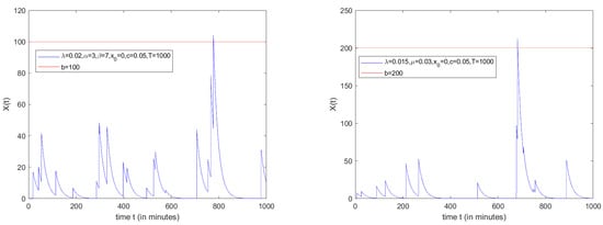
Figure 2. Left side: Numerical simulation of the process ${\left\{X(t)\right\}}_{t\ge 0}$, where $\lambda =0.02, \alpha =3,$ $\beta =7,$ $x_0=0,c=0.05$, $T=1000,$ (blue color), and congestion threshold $b=100$ (red color). Right side: Numerical simulation of the process ${\left\{X(t)\right\}}_{t\ge 0}$, where $\lambda =0.015, \mu =0.03, x_0=0,c=0.05, T=1000$ (blue color), and congestion threshold $b=200$ (red color).

Figure 3 gives a 3D illustration of the probability of the first passage time for our process ${\left\{X(t)\right\}}_{t\ge 0}$ to exceed a given congestion threshold with an exact simulation method, and a 3D illustration of the exponential approximation probability of the first passage time for our process ${\left\{X(t)\right\}}_{t\ge 0}$ to exceed a given congestion threshold. The simulations involved varying the incident clearance rate c and the time t. For the two specific cases given above, we have the following:

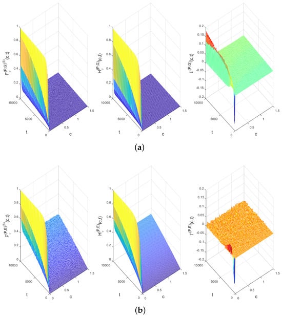
Figure 3. 3D illustration of the probability of the first passage time for our process to exceed a given congestion threshold using two methods (exact simulation and exponential approximation), with their deviations. (a) Numerical calculus of $F_{\tau }^{{(P,G)}^{(S)}}(c,t)$, $H_{\tau }^{(P,G)}(c,t)$ and ${\displaystyle {\Gamma }^{(P,G)}(c,t)}$, where $x_0=0, \lambda =0.02,$ $\alpha =3, \beta =7,$ $b=100$. (b) Numerical calculus of $F_{\tau }^{{(P,E)}^{(S)}}(c,t)$, $H_{\tau }^{(P,E)}(c,t)$ and ${\displaystyle {\Gamma }^{(P,E)}(c,t)}$, where $x_0=0, \lambda =0.015,$ $\mu =0.03, b=200$.

• Instead of $F_{\tau }^{{(P,G)}^{(S)}}(t)$ and $F_{\tau }^{{(P,E)}^{(S)}}(t)$, we denote, respectively, $F_{\tau }^{{(P,G)}^{(S)}}(c,t)$ and $F_{\tau }^{{(P,G)}^{(S)}}(c,t)$.
• Instead of $H_{\tau }^{(P,G)}(t)$ (see (18)) and $H_{\tau }^{(P,E)}(t)$ (see (22)), we denote, respectively, $H_{\tau }^{(P,G)}(c,t)$ and $H_{\tau }^{(P,E)}(c,t)$.

We then present the deviation between the calculation of the probabilities with the 3D illustrations, and those presented by the calculation of ${\displaystyle {\Gamma }^{(P,G)}(c,t)=F_{\tau }^{{(P,G)}^{(S)}}(c,t)-H_{\tau }^{(P,G)}(c,t)}$ and ${\displaystyle {\Gamma }^{(P,E)}(c,t)=F_{\tau }^{{(P,E)}^{(S)}}(c,t)-H_{\tau }^{(P,E)}(c,t)}$.

5. Applications

In this part, we give some interesting applications for the time needed for the free flow recovery process on a part of a road network. We consider that $b>max(x_0,m_X)$, where ${\displaystyle m_X=\frac{\lambda }{c}\mathbb{E}(W_i)}$ is the expected value of time needed for free flow recovery on infinite time-horizon (stationary expected value), and hence, $c\to 0$ and $b\to \infty$; see Definition 1.

5.1. Determination of Approximate Minimum Value of Incident Clearance Rate Needed to Limit Congestion Level with Respect to Given Probability

We do not provide in this work the exact expression of the probability of the first passage time for our process ${\left\{X(t)\right\}}_{t\ge 0}$ to exceed a given congestion threshold $F_{\tau }(t)$. Instead, we propose an analytic approximation, denoted as $H_{\tau }(t)$; see Proposition 1. We determine in this subsection the approximate minimum value of the incident clearance rate needed to limit a given congestion level with respect to a given probability. To obtain this approximate minimum value, we rely on historical data sets where the incident occurrence process follows a homogeneous Poisson distribution with intensity $\lambda$, and the increases in the time needed for free flow recovery after incident occurrences are gamma distributed with two parameters $\alpha$ and $\beta$, or exponentially distributed with intensity $\mu$. In order to place greater emphasis on the incident clearance rate, noted c, we emphasize its central role in the following analysis: Instead of the two probabilities $F_{\tau }(t)$ (see (6) or (7)) and $H_{\tau }(t)$ (see (12) in Proposition 1), we denote, respectively, $F_{\tau }(x_0,b,c,t)$ and $H_{\tau }(x_0,b,c,t)$. We also denote ${\displaystyle {\mathbb{E}}_{x_0,b,c}(\tau )}$ instead of ${\mathbb{E}}_{x_0}(\tau )$. Instead of the two specific approximate probabilities $H_{\tau }^{(P,G)}(t)$ (see (18) in Remark 1) and $H_{\tau }^{(P,E)}(t)$ (see (22) in Remark 2), we denote, respectively, $H_{\tau }^{(P,G)}(x_0,b,c,t)$ and $H_{\tau }^{(P,E)}(x_0,b,c,t)$. Also, instead of the two specific approximate expected values ${\mathbb{E}}_{x_0}^{(P,G)}(\tau )$ (see (16) in Remark 1) and ${\mathbb{E}}_{x_0}^{(P,E)}(\tau )$ (see for example (21)) in Remark 2), we denote, respectively, ${\mathbb{E}}_{x_0,b,c}^{(P,G)}(\tau )$ and ${\mathbb{E}}_{x_0,b,c}^{(P,E)}(\tau )$. Therefore, we have the following proposition:

Proposition 2. 

The probabilities $F_{\tau }(x_0,b,c,t)$ and $H_{\tau }(x_0,b,c,t)$ are decreasing with respect to c.

Proof. 

For $F_{\tau }(x_0,b,c,t)$, we have the following: By adopting the same direct proof of Proposition 2 from [1] (with the only difference here being consideration of the process ${\left\{X(t)\right\}}_{t\ge 0}$ (given by (3) or (4))).

For $H_{\tau }(x_0,b,c,t)$, we have

$${\displaystyle \frac{\partial H_{\tau }(x_0,b,c,t)}{\partial c}}=-{\displaystyle \frac{t}{{\displaystyle {\mathbb{E}}_{x_0,b,c}{(\tau )}^2}}}{\displaystyle \frac{{\displaystyle \partial {\mathbb{E}}_{x_0,b,c}(\tau )}}{\partial c}}exp\left(-{\displaystyle \frac{t}{{\displaystyle {\mathbb{E}}_{x_0,b,c}(\tau )}}}\right)<0,$$

where ${\displaystyle \frac{{\displaystyle \partial {\mathbb{E}}_{x_0,b,c}(\tau )}}{\partial c}>0}$ with the fact that $c>{\displaystyle \frac{\lambda }{b}}\mathbb{E}(W_i)$, and as $b\to \infty ,c\to 0$; see Definition 1.

Specifically, for the approximate probabilities $H_{\tau }^{(P,G)}(x_0,b,c,t)$ and $H_{\tau }^{(P,E)}(x_0,b,c,t)$, we have the following:

• ${\displaystyle \frac{\partial H_{\tau }^{(P,G)}(x_0,b,c,t)}{\partial c}<0}$ where ${\displaystyle \frac{{\displaystyle \partial {\mathbb{E}}_{x_0,b,c}^{(P,G)}(\tau )}}{\partial c}>0}$ with particular regard to the fact that $c>{\displaystyle \frac{\lambda }{b}}\alpha \beta$, and as $b\to \infty ,c\to 0$; see Definition 1.
• ${\displaystyle \frac{\partial H_{\tau }^{(P,E)}(x_0,b,c,t)}{\partial c}<0}$ where ${\displaystyle \frac{{\displaystyle \partial {\mathbb{E}}_{x_0,b,c}^{(P,E)}(\tau )}}{\partial c}>0}$, with particular regard to the fact that $c>{\displaystyle \frac{\lambda }{b\mu }}$, and as $b\to \infty ,c\to 0$; see Definition 1.

□

5.1.1. Analysis over Finite Time Horizon

The purpose of the analysis in this subsection is to determine the approximate minimum value of the incident clearance rate needed to avoid a given congestion threshold b with a given probability p. This minimum value is approximated as ${\displaystyle \tilde{c}(x_0,b,p,t)}$ and is given as follows:

$${\displaystyle \tilde{c}(x_0,b,p,t)=H_{\tau }^{-1}(x_0,b,p,t):=min\left\{c>\frac{\lambda }{b}\mathbb{E}(W_i),H_{\tau }(x_0,b,c,t)\le 1-p\right\},}$$

(23)

where ${\displaystyle H_{\tau }^{-1}(x_0,b,p,t)}$ is the pseudo-inverse of $H_{\tau }(x_0,b,c,t)$.

Two specific cases are presented as follows, where the following hold:

• The incident occurrences process is Poisson with intensity $\lambda$ and the increases in the time needed for free flow recovery after incident occurrences are gamma distributed with two parameters $\alpha$ and $\beta$. In this specific case, the approximate value of the minimum incident clearance rate is denoted by ${\displaystyle {\tilde{c}}^{(P,G)}(x_0,b,p,t)}$ and is given as follows:

  $${\displaystyle {\tilde{c}}^{(P,G)}(x_0,b,p,t)=H_{\tau }^{{-1}_{(P,G)}}(x_0,b,p,t):=min\left\{c>\frac{\lambda \alpha \beta }{b},H_{\tau }^{(P,G)}(x_0,b,c,t)\le 1-p\right\},}$$

  (24)

  where ${\displaystyle H_{\tau }^{{-1}_{(P,G)}}(x_0,b,p,t)}$ is the pseudo-inverse of $H_{\tau }^{(P,G)}(x_0,b,c,t)$.
• The incident occurrences process is Poisson with intensity $\lambda$ and the increases in the time needed for free flow recovery after incident occurrences are exponential distributed with intensity $\mu$. In this specific case, the approximate value of the minimum incident clearance rate is denoted by ${\displaystyle {\tilde{c}}^{(P,E)}(x_0,b,p,t)}$, and is as follows:

  $${\displaystyle {\tilde{c}}^{(P,E)}(x_0,b,p,t)=H_{\tau }^{{-1}_{(P,E)}}(x_0,b,p,t):=min\left\{c>\frac{\lambda }{b\mu },H_{\tau }^{(P,E)}(x_0,b,c,t)\le 1-p\right\},}$$

  (25)

  where $H_{\tau }^{{-1}_{(P,E)}}(x_0,b,p,t)$ is the pseudo-inverse of $H_{\tau }^{(P,E)}(x_0,b,c,t)$.

The analytic formula of the approximate minimum value ${\displaystyle \tilde{c}(x_0,b,p,t)}$ is not derived. Specifically, the analytic formulas approximate minimum values ${\displaystyle {\tilde{c}}^{(P,G)}(x_0,b,p,t)}$ and ${\displaystyle {\tilde{c}}^{(P,E)}(x_0,b,p,t)}$ are not derived. However, $H_{\tau }(x_0,b,c,t)$ is decreasing with respect to c; $(c>{\displaystyle \frac{\lambda }{b}}\mathbb{E}(W_i)$. This also applies to two special cases: (1) $H_{\tau }^{(P,G)}(x_0,b,c,t)$ is decreasing with respect to c; ($c>{\displaystyle \frac{\lambda }{b}}\alpha \beta$), and (2) $H_{\tau }^{(P,E)}(x_0,b,c,t)$ is decreasing with respect to c ($c>{\displaystyle \frac{\lambda }{b\mu }}$); see Proposition 2. We propose here to calculate numerically the two approximate minimum values ${\displaystyle {\tilde{c}}^{(P,G)}(x_0,b,p,t)}$ and ${\displaystyle {\tilde{c}}^{(P,E)}(x_0,b,p,t)}$ by employing one of the following algorithms: dichotomy, Fibonnacci, or the gold number.

5.1.2. Description of Data Sets

We present in this subsection two data sets:

• For the first data set, we describe the incident data collected in [24] for the morning and evening peak periods (7:00–10:00 a.m. and 4:00–7:00 p.m.), from 1 January 2003 to 30 April 2003, on the southbound I-405, Seattle, Washington. We present some data metrics in Table 1 concerning the number of incidents and the increases in the time needed for free flow recovery after incident occurrences. Various continuous and discrete distributions were tested to fit the increases in the time needed for free flow recovery after incident occurrences and the number of incidents, respectively. Parameters were obtained using Maximum Likelihood Estimation (MLE). Goodness-of-fit tests (Kolmogorov-Smirnov, Anderson-Darling, and Chi-squared) indicate that a gamma distribution with parameters $\alpha =2.14026$ and $\beta =7.83599$ best fits the increases in the time needed for free flow recovery after incident occurrences, while a Poisson distribution with parameter $\lambda =5.0119$ per 6 h of time period best fits the number of incident occurrences. These results are shown in Figure 4.
  Table 1. Summary of metrics for the number of incidents and the increases in the time needed for free flow recovery after incident occurrences data.

  Data Types
  Number of incidents data		Increases in the time needed for free flow recovery after incident occurrences data
  Metrics	Value	Metrics	Value
  Sample size	84	Sample size	84
  Min	1	Min	1
  Mean	5.0119	Mean	16.7710
  Std. Deviation	2.8770	Std. Deviation	10.7241
  Coef. of variation	0.5740	Coef. of variation	0.6394
  Std. Error	0.3139	Std. Error	1.1701
  Skewness	1.2493	Skewness	1.0395
  Max	15	Max	54

  

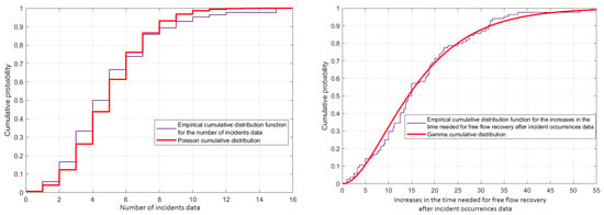  Figure 4. Left side: Empirical cumulative distribution function for the number of incidents data fitted by a Poisson cumulative distribution function with intensity $\lambda =5.0119$ per 6 h of the time period. Right side: Empirical cumulative distribution function for the increases in the time needed for free flow recovery after incident occurrences data fitted by a gamma cumulative distribution function with the two parameters $\alpha =2.14026$ and $\beta =7.83599$.
• For the second data set, it is described in [1] for a 1 km freeway segment of I-880 located in Hayward, Alameda County, California, USA, during the spring of 1993. The incident occurrences follow a homogeneous Poisson process with an intensity of $\lambda =0.00833$, and the increases in the time needed for free flow recovery after incident occurrences are modeled by an exponential distribution with an intensity of $\mu =0.04$.

5.1.3. Numerical Results

In this subsection, we give some significant numerical results from Example 1 and graphical illustrations. Two specific cases are discussed.

Example 1. 

From the two data sets described above, the following is considered:

• For the first case ${\tilde{c}}^{(P,G)}(x_0,b,p,t)$:
  • We take $\lambda =0.014$ (the intensity of incident occurrences process) and $\alpha =2.14026$ and $\beta =7.83599$ (the two parameters estimated for the gamma distribution of the increases in the time needed for free flow recovery after incident occurrences). By using Formula (24), we calculate the approximate values for the minimum clearance rate needed to avoid the congestion threshold b with respect to the probability p for the finite time horizons $t=7500$ and $t=15,000$. For instance, Figure 5a shows ${\tilde{c}}^{(P,G)}({\displaystyle \frac{b}{5}},b,p,t)$. Then, we have, for example, ${\tilde{c}}^{(P,G)}(20,100,0.85,7500)=0.016$ and ${\tilde{c}}^{(P,G)}(20,100,0.85,15,000)=0.0213$.
    

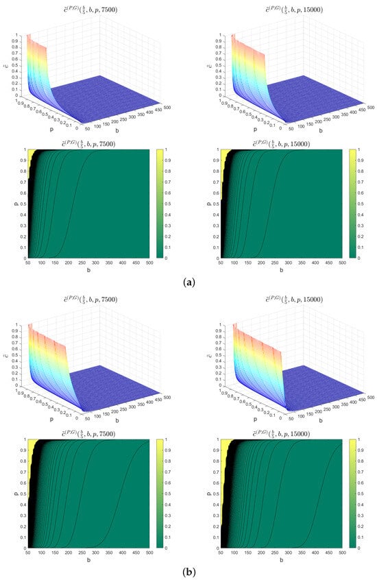    Figure 5. 3D illustration and contour lines of ${\tilde{c}}^{(P,G)}(x_0,b,p,t)$. (a) 3D illustration of ${\tilde{c}}^{(P,G)}(x_0={\displaystyle \frac{b}{5}},b,p,t=7500)$ (top left) with its contour lines (bottom left), and 3D illustration of ${\tilde{c}}^{(P,G)}(x_0={\displaystyle \frac{b}{5}},b,p,t=15,000)$ (top right) with its contour lines (bottom right), for $\lambda =0.014$, $\alpha =2.14026$ and $\beta =7.83599$. (b) 3D illustration of ${\tilde{c}}^{(P,G)}(x_0={\displaystyle \frac{b}{5}},b,p,t=7500)$ (top left) with its contour lines (bottom left), and 3D illustration of ${\tilde{c}}^{(P,G)}(x_0={\displaystyle \frac{b}{5}},b,p,t=15,000)$ (top right) with its contour lines (bottom right), for $\lambda =0.03$, $\alpha =2.14026$ and $\beta =7.83599$.
  • Instead of $\lambda =0.014$ (the intensity of incident occurrences process), we take $\lambda =0.03$. Similarly, we calculate the approximate values for the minimum clearance rate needed to avoid the congestion threshold b with respect to the probability p, for the finite time horizons $t=7500$ and $t=15,000$. Figure 5b shows ${\tilde{c}}^{(P,G)}({\displaystyle \frac{b}{5}},b,p,t)$. Then we have, for example, ${\tilde{c}}^{(P,G)}(20,100,0.85,7500)=0.0470$, and ${\tilde{c}}^{(P,G)}(20,100,0.85,15,000)=0.0642$.
• For the second case ${\tilde{c}}^{(P,E)}(x_0,b,p,t)$:
  • We take $\lambda =0.00833$ (the intensity of incident occurrences process) and $\mu =0.04$ (the intensity of the increases in the time needed for free flow recovery after incident occurrences). Using Formula (25), we calculate the approximate values for the minimum clearance rate needed to avoid the congestion threshold b with respect to the probability p for the finite time horizons $t=10,000$ and $t=20,000$. In Figure 6a, we present ${\tilde{c}}^{(P,E)}(0,b,p,10,000)$ and ${\tilde{c}}^{(P,E)}(0,b,p,20,000)$. Then, for example, we have ${\tilde{c}}^{(P,E)}(0,190,0.80,10,000)=0.0095$ and ${\tilde{c}}^{(P,E)}(0,180,0.8,20,000)=0.0180$.
    

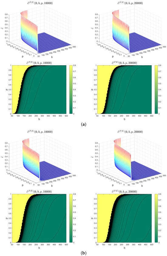    Figure 6. 3D illustration and contour lines of ${\tilde{c}}^{(P,E)}(x_0,b,p,t)$. (a) 3D illustration of ${\tilde{c}}^{(P,E)}(x_0=0,b,p,t=10,000)$ (top left) with its contour lines (bottom left), and 3D illustration of ${\tilde{c}}^{(P,E)}(x_0=0,b,p,t=20,000)$ (top right) with its contour lines (bottom right), for $\lambda =0.00833$, $\mu =0.04$. (b) 3D illustration of ${\tilde{c}}^{(P,E)}(x_0=0,b,p,t=10,000)$ (top left) with its contour lines (bottom left), and 3D illustration of ${\tilde{c}}^{(P,E)}(x_0=0,b,p,t=20,000)$ (top right) with its contour lines (bottom right), for $\lambda =0.02$, $\mu =0.04$.
  • Instead of $\lambda =0.00833$ (the intensity of incident occurrences process), we take $\lambda =0.02$. In the same way as the above instance, we calculate the approximate values for the minimum clearance rate needed to avoid the congestion threshold b with respect to the probability p for the finite time horizons $t=10,000$ and $t=20,000$. In Figure 6b, we show ${\tilde{c}}^{(P,E)}(0,b,p,10,000)$ and ${\tilde{c}}^{(P,E)}(0,b,p,20,000)$. Then, for example, we have ${\tilde{c}}^{(P,E)}(0,190,0.80,10,000)=0.0545$ and ${\tilde{c}}^{(P,E)}(0,180,0.8,20,000)=0.4443$.

5.1.4. Interpretation of Results

Figure 5 and Figure 6 show a 3D illustration and contour lines for two specific cases of the numerical presentation of the approximate minimum values of incident clearance rate, which we denoted, respectively, by ${\displaystyle {\tilde{c}}^{(P,G)}(x_0,b,p,t)}$ and ${\displaystyle {\tilde{c}}^{(P,E)}(x_0,b,p,t)}$. These approximate minimum values of the incident clearance rate are given as a function of the traffic congestion threshold b and the probability p. Following from Figure 5 and Figure 6 for the two specific cases presented with fixed two different finite times and initial states, we have the following comments: First, we observe that the approximate minimum values ${\displaystyle {\tilde{c}}^{(P,G)}(x_0,b,p,t)}$ and ${\displaystyle {\tilde{c}}^{(P,E)}(x_0,b,p,t)}$ increase with respect to the probability p, which can be interpreted as the fact that road operators prioritize a high level of assurance (reflected by a high value of p) in ensuring that the congestion threshold b is not surpassed; thus, they need to guarantee prompt incident resolution, and it is essential to step up efforts by allocating additional resources such as equipment, personnel, and other necessary means. Second, we can see that the approximate minimum values ${\displaystyle {\tilde{c}}^{(P,G)}(x_0,b,p,t)}$ and ${\displaystyle {\tilde{c}}^{(P,E)}(x_0,b,p,t)}$ decrease with respect to the congestion threshold b. This means that if road operators do not intend to exceed the low-level of congestion threshold b, they need to promptly address incidents by enhancing their efforts, such as deploying additional equipment, increasing staff numbers, etc. Third, we can see that the approximate minimum values ${\displaystyle {\tilde{c}}^{(P,G)}(x_0,b,p,t)}$ and ${\displaystyle {\tilde{c}}^{(P,E)}(x_0,b,p,t)}$ increase with respect to t. Similarly, if road operators aim to prevent the congestion threshold b from being exceeded for extended periods of time t, they must promptly address incidents by intensifying their efforts, which may involve deploying additional equipment, increasing staff numbers, and implementing other appropriate measures. Fourth, we can see that the approximate minimum values ${\displaystyle {\tilde{c}}^{(P,G)}(x_0,b,p,t)}$ and ${\displaystyle {\tilde{c}}^{(P,E)}(x_0,b,p,t)}$ increase due to an increase in the intensity of incident occurrences process and fixed parameters of the known distribution of the increases in the time needed for free flow recovery due to the incident occurrences (gamma or exponential distributions). The increase in these minimum values can be interpreted as the need for high level of assurance from the road operators that the congestion threshold b will not be reached. In order to achieve this, they must significantly increase their efforts in resolving incidents promptly. This could involve multiplying their resources, such as equipment and staff, dedicated to effectively managing and resolving incidents in a timely manner.

5.2. Determination of Approximate Maximum Intensity of Incident Occurrences Process Needed to Limit Congestion Level with Respect to Given Probability

As in Section 5.1, we do not provide the exact expression of the probability of the first passage time for our process ${\left\{X(t)\right\}}_{t\ge 0}$ to exceed a given congestion threshold $F_{\tau }(t)$. Instead, we propose an analytic approximation, denoted as $H_{\tau }(t)$; see Proposition 1. We determine in this subsection the approximate maximum intensity of the incident occurrences process needed to limit a given congestion level with a given probability. In order to determine the approximate maximum value of this intensity, our approximations will be based on historical data sets and the average values of the incident clearance rate. We estimate the parameters of the distributions of the increases in the time needed for free flow recovery after incident occurrences (gamma distributed with two parameters $\alpha$ and $\beta$, and exponential distribution with intensity $\mu$). As in Section 5.1, and in order to highlight the intensity of the incident occurrences process, denoted by $\lambda$, we consider the following: (1) Instead of the two probabilities $F_{\tau }(t)$ (see (6) or (7)) and $H_{\tau }(t)$ (see (12) in Proposition 1), we denote, respectively, $F_{\tau }(x_0,b,\lambda ,t)$ and $H_{\tau }(x_0,b,\lambda ,t)$. Instead of the two specific approximation probabilities $H_{\tau }^{(P,G)}(t)$ and $H_{\tau }^{(P,E)}(t)$ (see (18) in Remark 1 and (22) in Remark 2, respectively), we denote $H_{\tau }^{(G,c)}(x_0,b,\lambda ,t)$ instead of $H_{\tau }^{(P,G)}(t)$ and $H_{\tau }^{(E,c)}(x_0,b,\lambda ,t)$ instead of $H_{\tau }^{(P,E)}(t)$. We also denote ${\displaystyle {\mathbb{E}}_{x_0,b,\lambda }(\tau )}$ instead of ${\mathbb{E}}_{x_0}(\tau )$. We denote the expected values ${\displaystyle {\mathbb{E}}_{x_0,b,\lambda }^{(G,c)}(\tau )}$ and ${\displaystyle {\mathbb{E}}_{x_0,b,\lambda }^{(E,c)}(\tau )}$ instead of ${\displaystyle {\mathbb{E}}_{x_0}^{(P,G)}(\tau )}$ and ${\displaystyle {\mathbb{E}}_{x_0}^{(P,E)}(\tau )}$. Therefore, we have the following proposition:

Proposition 3. 

The two probabilities $F_{\tau }(x_0,b,\lambda ,t)$ and $H_{\tau }(x_0,b,\lambda ,t)$ are increasing with respect to λ.

Proof. 

For $F_{\tau }(x_0,b,\lambda ,t)$, we adopt the same proof of Proposition 4 from [1] (with consideration of the process ${\left\{X(t)\right\}}_{t\ge 0}$ (given (3) or (4)) here).

For $H_{\tau }(x_0,b,\lambda ,t)$, we have the following:

$${\displaystyle \frac{\partial H_{\tau }(x_0,b,\lambda ,t)}{\partial \lambda }}=-{\displaystyle \frac{t}{{\displaystyle {\mathbb{E}}_{x_0,b,\lambda }{(\tau )}^2}}}{\displaystyle \frac{{\displaystyle \partial {\mathbb{E}}_{x_0,b,\lambda }(\tau )}}{\partial \lambda }}exp\left(-{\displaystyle \frac{t}{{\displaystyle {\mathbb{E}}_{x_0,b,\lambda }(\tau )}}}\right)>0,$$

where ${\displaystyle \frac{{\displaystyle \partial {\mathbb{E}}_{x_0,b,\lambda }(\tau )}}{\partial \lambda }<0}$, with the fact that $0<\lambda <{\displaystyle \frac{cb}{\mathbb{E}(W_i)}}$, and as $b\to \infty ,c\to 0$; see Definition 1.

Specifically, for the approximate probabilities $H_{\tau }^{(G,c)}(x_0,b,\lambda ,t)$ and $H_{\tau }^{(E,c)}(x_0,b,\lambda ,t)$, we have the following:

• ${\displaystyle \frac{\partial H_{\tau }^{(G,c)}(x_0,b,\lambda ,t)}{\partial \lambda }>0}$ where ${\displaystyle \frac{{\displaystyle \partial {\mathbb{E}}_{x_0,b,\lambda }^{(G,c)}(\tau )}}{\partial \lambda }<0}$ with the fact that $0<\lambda <{\displaystyle \frac{cb}{\alpha \beta }}$, and as $b\to \infty ,c\to 0$; see Definition 1.
• ${\displaystyle \frac{\partial H_{\tau }^{(E,c)}(x_0,b,\lambda ,t)}{\partial \lambda }>0}$ where ${\displaystyle \frac{{\displaystyle \partial {\mathbb{E}}_{x_0,b,\lambda }^{(E,c)}(\tau )}}{\partial \lambda }<0}$ with the fact that $0<\lambda <cb\mu$, and as $b\to \infty ,c\to 0$; see Definition 1.

□

5.2.1. Analysis over Finite Time Horizon

The aim of the analysis in this subsection is to find the approximate maximum value of the incident occurrences process needed to avoid a given congestion threshold b with a given probability p. The approximate maximum value of the incident occurrences process is defined as ${\displaystyle \tilde{\lambda }(x_0,b,p,t)}$ and is given as follows:

$${\displaystyle \tilde{\lambda }(x_0,b,p,t)=H_{\tau }^{-1}(x_0,b,p,t):=max\left\{0<\lambda <\frac{bc}{\mathbb{E}(W_i)},H_{\tau }(x_0,b,\lambda ,t)\le 1-p\right\},}$$

(26)

where ${\displaystyle H_{\tau }^{-1}(x_0,b,p,t)}$ is the pseudo-inverse of $H_{\tau }(x_0,b,\lambda ,t)$.

Two cases are distinguished:

• The increases in the time needed for free flow recovery after incident occurrences are gamma distributed with two parameters $\alpha$ and $\beta$, and the incident clearance rate is modeled with the constant c. In this specific case, the approximate maximum value is denoted by ${\displaystyle {\tilde{\lambda }}^{(G,c)}(x_0,b,p,t)}$, and is as follows:

  $$\begin{array}{cc}\hfill {\displaystyle {\tilde{\lambda }}^{(G,c)}(x_0,b,p,t)}& =H_{\tau }^{{-1}_{(G,c)}}(x_0,b,p,t)\hfill \\ \hfill & :=max\left\{0<\lambda <{\displaystyle \frac{bc}{\alpha \beta }},H_{\tau }^{(G,c)}(x_0,b,\lambda ,t)\le 1-p\right\},\hfill \end{array}$$

  (27)

  where ${\displaystyle H_{\tau }^{{-1}_{(G,c)}}(x_0,b,p,t)}$ is the pseudo-inverse of $H_{\tau }^{(G,c)}(x_0,b,\lambda ,t)$.
• The increases in the time needed for free flow recovery after incident occurrences are exponentially distributed with intensity $\mu$, and the incident clearance rate is modeled with the constant c. In this specific case, the approximate maximum value is denoted by ${\displaystyle {\tilde{\lambda }}^{(E,c)}(x_0,b,p,t)}$, and is as follows:

  $$\begin{array}{cc}\hfill {\displaystyle {\tilde{\lambda }}^{(E,c)}(x_0,b,p,t)}& =H_{\tau }^{{-1}_{(E,c)}}(x_0,b,p,t)\hfill \\ & :=max\left\{0<\lambda <bc\mu ,H_{\tau }^{(E,c)}(x_0,b,\lambda ,t)\le 1-p\right\},\hfill \end{array}$$

  (28)

  where $H_{\tau }^{{-1}_{(E,c)}}(x_0,b,p,t)$ is the pseudo-inverse of $H_{\tau }^{(E,c)}(x_0,b,\lambda ,t)$.

The analytic formula of approximate maximum value ${\displaystyle \tilde{\lambda }(x_0,b,p,t)}$ is not derived. Specifically, the analytic formulas of approximate maximum values ${\displaystyle {\tilde{\lambda }}^{(G,c)}(x_0,b,p,t)}$ and ${\displaystyle {\tilde{\lambda }}^{(E,c)}(x_0,b,p,t)}$ are not derived. However, $H_{\tau }(x_0,b,\lambda ,t)$ is increasing with respect to $\lambda$; ($0<\lambda <{\displaystyle \frac{cb}{\mathbb{E}(W_i)}}$). This also applies to two special cases: (1) $H_{\tau }^{(G,c)}(x_0,b,\lambda ,t)$ is increasing with respect to $\lambda$—$0<\lambda <{\displaystyle \frac{cb}{\alpha \beta }}$; and (2) $H_{\tau }^{(E,c)}(x_0,b,\lambda ,t)$ is increasing with respect to $\lambda$; ($0<\lambda <cb\mu$) (see Proposition 3). We propose here to compute the two approximate maximum values ${\displaystyle {\tilde{\lambda }}^{(G,c)}(x_0,b,p,t)}$ and ${\displaystyle {\tilde{\lambda }}^{(E,c)}(x_0,b,p,t)}$ numerically, using algorithms such as dichotomy, Fibonnacci, or the gold number.

5.2.2. Numerical Results

We propose in this part for this second application Example 2 accompanied by graphical illustrations. Two special cases are dealt with.

Example 2. 

• For the first specific case ${\tilde{\lambda }}^{(G,c)}(x_0,b,p,t)$:

  1. 

  We take $c=0.1$ (the incident clearance rate), and $\alpha =5$ and $\beta =8$ (the two parameters for the gamma distribution of the increases in the time needed for free flow recovery after incident occurrences). By using Formula (27), we calculate the approximate values for the maximum intensity of the incident occurrences process needed to avoid the congestion threshold b with respect to the probability p, for the finite time horizons $t=7500$ and $t=15,000$. Figure 7a presents ${\tilde{\lambda }}^{(G,c)}(0,b,p,7500)$ and ${\tilde{\lambda }}^{(G,c)}(0,b,p,15,000)$. We also have ${\tilde{\lambda }}^{(G,c)}(0,180,0.99,7500)=0.0228$ and ${\tilde{\lambda }}^{(G,c)}(0,180,0.99,15,000)=0.0188$.

  

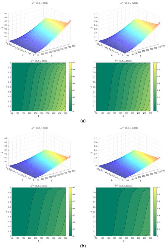  Figure 7. 3D illustration and contour lines of ${\tilde{\lambda }}^{(G,c)}(x_0,b,p,t)$. (a) 3D illustration of ${\tilde{\lambda }}^{(G,c)}(x_0=0,b,p,t=7500)$ (top left) with its contour lines (bottom left), and 3D illustration of ${\tilde{\lambda }}^{(G,c)}(x_0=0,b,p,t=15,000)$ (top right) with its contour lines (bottom right), for $c=0.1$, $\alpha =8$, and $\beta =5$. (b) 3D illustration of ${\tilde{\lambda }}^{(G,c)}(x_0=0,b,p,t=7500)$ (top left) with its contour lines (bottom left), and 3D illustration of ${\tilde{\lambda }}^{(G,c)}(x_0=0,b,p,t=15,000)$ (top right) with its contour lines (bottom right), for $c=0.05$, $\alpha =8$, and $\beta =5$.

  2. 

  Instead of $c=0.1$ (the incident clearance rate), we take $c=0.05$. In the same way as in the first instance, we calculate the approximate values for the maximum intensity of the incident occurrences process needed to avoid the congestion threshold b with respect to the probability p, for the finite time horizons $t=7500$ and $t=15,000$. Figure 7b illustrates ${\tilde{\lambda }}^{(G,c)}(0,b,p,7500)$ and ${\tilde{\lambda }}^{(G,c)}(0,b,p,15,000)$. We also have ${\tilde{\lambda }}^{(G,c)}(0,180,0.99,7500)=0.0137$ and ${\tilde{\lambda }}^{(G,c)}(0,180,0.99,15,000)=0.0114$.

• For the second specific case ${\tilde{\lambda }}^{(E,c)}(x_0,b,p,t)$:

  1. 

  We take $c=1/7$ (the incident clearance rate) and $\mu =1/30$ (the intensity of the increases in the time needed for free flow recovery after incident occurrences). By using Formula (28), we calculate the approximate values for the maximum intensity of the incident occurrences process needed to avoid the congestion threshold b with respect to the probability p, for the finite time horizons $t=10,000$ and $t=20,000$. In Figure 8a, we present ${\tilde{\lambda }}^{(E,c)}(b/5,b,p,10,000)$ and ${\tilde{\lambda }}^{(E,c)}(b/5,b,p,20,000)$. Then, for example, we have ${\tilde{\lambda }}^{(E,c)}(50,250,0.85,10,000)=0.0368$, and ${\tilde{\lambda }}^{(E,c)}(50,250,0.85,20,000)=0.0229$.

  

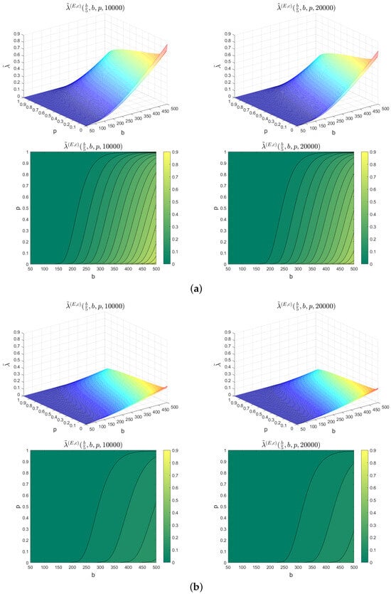  Figure 8. 3D illustration and contour lines of ${\tilde{\lambda }}^{(E,c)}(x_0,b,p,t)$. (a) 3D illustration of ${\tilde{\lambda }}^{(E,c)}(x_0={\displaystyle \frac{b}{5}},b,p,t=10,000)$ (top left) with its contour lines (bottom left), and 3D illustration of ${\tilde{\lambda }}^{(E,c)}(x_0={\displaystyle \frac{b}{5}},b,p,t=20,000)$ (top right) with its contour lines (bottom right), for $c=1/7$, $\mu =1/30$. (b) 3D illustration of ${\tilde{\lambda }}^{(E,c)}(x_0={\displaystyle \frac{b}{5}},b,p,t=10,000)$ (top left) with its contour lines (bottom left), and 3D illustration of ${\tilde{\lambda }}^{(E,c)}(x_0={\displaystyle \frac{b}{5}},b,p,t=20,000)$ (top right) with its contour lines (bottom right), for $c=0.03$, $\mu =1/30$.

  2. 

  Instead of $c=1/7$ (the incident clearance rate), we take $c=0.03$. In the same way as in the second instance, we calculate the approximate values for the maximum intensity of incident occurrences process needed to avoid the congestion threshold b with respect to the probability p, for the finite time horizons $t=10,000$ and $t=20,000$. In Figure 8b, we also present for this instance ${\tilde{\lambda }}^{(E,c)}(b/5,b,p,10,000)$ and ${\tilde{\lambda }}^{(E,c)}(b/5,b,p,20,000)$. Then, for example, we have ${\tilde{\lambda }}^{(E,c)}(50,250,0.85,10,000)=0.0182$ and ${\tilde{\lambda }}^{(E,c)}(50,250,0.85,20,000)=0.0129$.

5.2.3. Interpretation of Results

Figure 7 and Figure 8 show 3D illustrations and contour lines for two specific cases of the numerical approximations of the maximum values of the intensity of the incident occurrences process, which we denoted, respectively, by ${\displaystyle {\tilde{\lambda }}^{(G,c)}(x_0,b,p,t)}$ and ${\displaystyle {\tilde{\lambda }}^{(G,c)}(x_0,b,p,t)}$. These approximate maximum values of the intensity of the incident occurrences process are given as functions of the traffic congestion threshold b and probability p for the two specific cases presented with two different finite horizon times and initial states. Then, we have the following comments: First, we observe that the approximate maximum values ${\displaystyle {\tilde{\lambda }}^{(G,c)}(x_0,b,p,t)}$ and ${\displaystyle {\tilde{\lambda }}^{(E,c)}(x_0,b,p,t)}$ decrease with respect to the probability p, which implies that for road operators, in order to have a high level of assurance (represented with a high value of p) that the congestion threshold b will not be surpassed, they should aim for low values of the approximate maximum intensity of the incident occurrences process. Lower values of the approximate maximum average incident count will contribute to maintaining the desired level of assurance. Second, we observe that the approximate maximum values ${\displaystyle {\tilde{\lambda }}^{(G,c)}(x_0,b,p,t)}$ and ${\displaystyle {\tilde{\lambda }}^{(E,c)}(x_0,b,p,t)}$ increase with respect to the congestion threshold b, which indicates that for road operators, in order to have a high level of assurance that the congestion threshold b will not be exceeded, it is necessary to reduce the approximate maximum intensity of the incident occurrences process. By decreasing the approximate maximum average values of the incident count, road operators can enhance their level of assurance. Third, we observe that the approximate maximum values ${\displaystyle {\tilde{\lambda }}^{(G,c)}(x_0,b,p,t)}$ and ${\displaystyle {\tilde{\lambda }}^{(E,c)}(x_0,b,p,t)}$ decrease with respect to time t. Similarly, if road operators aim to guarantee that the congestion threshold b is not surpassed for extended periods of time t, they should also strive for a low approximate intensity of the incident occurrence process. By achieving a lower approximate maximum value of the incident count, road operators can enhance their ability to prevent the congestion threshold from being exceeded over longer times. Fourth, we observe that the approximate maximum values ${\displaystyle {\tilde{\lambda }}^{(G,c)}(x_0,b,p,t)}$ and ${\displaystyle {\tilde{\lambda }}^{(E,c)}(x_0,b,p,t)}$ increase due to the increase in the incident clearance rate c and fixed the intensity of the increases in the time needed for free flow recovery after incident occurrences $\mu$. This means that for road operators to have a high level of assurance that the congestion threshold b will not be exceeded, they should increase their efforts in incident resorption, for example, by increasing the incident clearance rate. This will lead to higher values of the approximate maximum intensity of the incident occurrence process for the two specific cases. Consequently, the approximate maximum values of the resorted incident count will also be high.

5.3. Determination of Approximate Minimum Value of Intensity of Increases in Time Needed for Free Flow Recovery After Incident Occurrences $\mu$ Needed to Limit Given Congestion Level with Respect to Given Probability

As in Section 5.1 and Section 5.2, we use in this subsection the analytic approximation probability of the first passage time for our process ${\left\{X(t)\right\}}_{t\ge 0}$ to exceed a given congestion threshold (which we denoted by $H_{\tau }(t)$; see Proposition 1). We determine the approximate minimum intensity of the increases in the time needed for free flow recovery after incident occurrences while avoiding a given congestion threshold with respect to a given probability. In order to find this minimum value, we base our approximation on historical data sets. The incident occurrences process is homogeneous Poisson with intensity $\lambda$, while the average value of the incident clearance rate is modeled with a constant c. In order to place greater emphasis on the intensity of the increases in the time needed for free flow recovery after incident occurrences, noted $\mu$, we emphasize its central role in the following analysis: Instead of denoting the two probabilities $F_{\tau }(t)$ (see (6) or (7)) and $H_{\tau }(t)$ (see (12) in Proposition 1), we denote, respectively, $F_{\tau }(x_0,b,\mu ,t)$ and $H_{\tau }(x_0,b,\mu ,t)$. In addition, instead of denoting the probability $H_{\tau }^{P,E}(t)$ (see (22) in Remark 2), we denote $H_{\tau }^{(P,c)}(x_0,b,\mu ,t)$. Instead of denoting ${\mathbb{E}}_{x_0}^{(P,E)}(\tau )$ (see, for example, (21) in Remark 2) we denote ${\displaystyle {\mathbb{E}}_{x_0,b,\mu }^{(P,c)}(\tau )}$. Therefore, we have the following proposition:

Proposition 4. 

The probabilities $F_{\tau }(x_0,b,\mu ,t)$ and, $H_{\tau }(x_0,b,\mu ,t)$ (i.e., $H_{\tau }^{(P,c)}(x_0,b,\mu ,t)$) are decreasing with respect to μ.

Proof. 

For $F_{\tau }(x_0,b,\mu ,t)$, we adopt the proof of Proposition 6 from [1] (with consideration of the process ${\left\{X(t)\right\}}_{t\ge 0}$ (given (3) or (4)) here).

For $H_{\tau }^{P,c}(x_0,b,\mu ,t)$, we have

$${\displaystyle \frac{\partial H_{\tau }^{(P,c)}(x_0,b,\mu ,t)}{\partial \mu }}=-{\displaystyle \frac{t}{{\displaystyle {\mathbb{E}}_{x_0,b,\mu }^{(P,c)}{(\tau )}^2}}}{\displaystyle \frac{{\displaystyle \partial {\mathbb{E}}_{x_0,b,\mu }^{(P,c)}(\tau )}}{\partial \mu }}exp\left(-{\displaystyle \frac{t}{{\displaystyle {\mathbb{E}}_{x_0,b,\mu }^{(P,c)}(\tau )}}}\right)<0,$$

where ${\displaystyle \frac{{\displaystyle \partial {\mathbb{E}}_{x_0,b,\mu }^{(P,c)}(\tau )}}{\partial \mu }>0}$, by bearing in mind that $0<\mathbb{E}(W_i)={\displaystyle \frac{1}{\mu }}<{\displaystyle \frac{cb}{\lambda }}$, and as $b\to \infty ,c\to 0$; see Definition 1. □

5.3.1. Analysis over Finite Time Horizon

The aim of the analysis in this subsection is to determine the approximate minimum intensity of the increases in the time needed for free flow recovery after incident occurrences, denoted ${\displaystyle \tilde{\mu }(x_0,b,p,t)}$, necessary to avoid a given congestion threshold b with a given probability p. We consider the case where the incident occurrences process is Poisson, and the incident clearance rate is modeled with a constant c. In this specific case, the approximate value of the minimum intensity of the increases in the time needed for free flow recovery after incident occurrences is denoted by ${\displaystyle {\tilde{\mu }}^{(P,c)}(x_0,b,p,t)}$, and is given as follows:

$$\begin{array}{cc}\hfill {\displaystyle {\tilde{\mu }}^{(P,c)}(x_0,b,p,t)}& =H_{\tau }^{{-1}_{(P,c)}}(x_0,b,p,t)\hfill \\ & :=min\left\{0<\mathbb{E}(W_i)={\displaystyle \frac{1}{\mu }}<{\displaystyle \frac{bc}{\lambda }},H_{\tau }^{(P,c)}(x_0,b,\mu ,t)\le 1-p\right\},\hfill \end{array}$$

(29)

where ${\displaystyle H_{\tau }^{{-1}_{(P,c)}}(x_0,b,p,t)}$ is the pseudo-inverse of $H_{\tau }^{(P,c)}(x_0,b,\mu ,t)$.

The approximate minimum ${\displaystyle {\tilde{\mu }}^{(P,c)}(x_0,b,p,t)}$ is not given analytically. However, as $H_{\tau }^{(P,c)}(x_0,b,\mu ,t)$ is decreasing with respect to $\mu$; ($0<{\displaystyle \frac{1}{\mu }}<{\displaystyle \frac{cb}{\lambda }}$) (see Proposition 4), we can compute numerically ${\displaystyle {\tilde{\mu }}^{(P,c)}(x_0,b,p,t)}$ using one of the following algorithms: dichotomy, Fibonnacci, or the gold number.

5.3.2. Numerical Results

We propose in this part for this third application Example 3 accompanied by graphical illustrations, where we take the same values given in Table 3 (from [12] the two values f and r). Only one special case is covered.

Example 3. 

For ${\tilde{\mu }}^{(P,c)}(x_0,b,p,t)$:

• We take $c=0.3$ (the incident clearance rate) and $\lambda =0.012$ (the intensity of the incident occurrences process). By using Formula (29), we calculate the approximate values for the minimum intensity of the increases in the time needed for free flow recovery after incident occurrences needed to avoid the congestion threshold b with respect to probability p for the finite time horizons $t=10,000$, and $t=20,000$. Figure 9a presents ${\tilde{\mu }}^{(P,c)}(0,b,p,10,000)$ and ${\tilde{\mu }}^{(P,c)}(0,b,p,20,000)$. We also have ${\tilde{\mu }}^{(P,c)}(0,120,0.70,10,000)=0.0492$ and ${\tilde{\mu }}^{(P,c)}(0,120,0.70,20,000)=0.0550$.
  

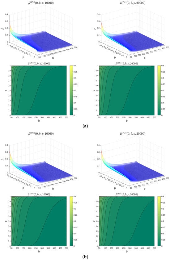  Figure 9. 3D illustration and contour lines of ${\tilde{\mu }}^{(P,c)}(x_0,b,p,t)$. (a) 3D illustration of ${\tilde{\mu }}^{(P,c)}(x_0=0,b,p,t=10,000)$ (top left) with its contour lines (bottom left), and 3D illustration of ${\tilde{\mu }}^{(P,c)}(x_0=0,b,p,t=20,000)$ (top right) with its contour lines (bottom right), for $c=0.3$, $\lambda =0.012$. (b) 3D illustration of ${\tilde{\mu }}^{(P,c)}(x_0=0,b,p,t=10,000)$ (top left) with its contour lines (bottom left), and 3D illustration of ${\tilde{\mu }}^{(P,c)}(x_0=0,b,p,20,000)$ (top right) with its contour lines (bottom right), for $c=0.015$, $\lambda =0.012$.
• Let us take $c=0.015$ instead of $c=0.3$ (the incident clearance rate). Figure 9b illustrates ${\tilde{\mu }}^{(P,c)}(0,b,p,10,000)$ and ${\tilde{\mu }}^{(P,c)}(0,b,p,20,000)$. We also have ${\tilde{\mu }}^{(P,c)}(0,120,0.70,10,000)=0.0612$ and ${\tilde{\mu }}^{(P,c)}(0,120,0.70,20,000)=0.0678$.

5.3.3. Interpretation of Results

Figure 9 shows 3D illustrations and contour lines for the approximate minimum value of the intensity of the increases in the time needed for free flow recovery after incident occurrences, which we denoted by ${\displaystyle {\tilde{\mu }}^{(P,c)}(x_0,b,p,t)}$. This approximate minimum value is given as a function of the traffic congestion threshold b and the probability p. From Figure 9, and for the case presented with two different finite horizon times and initial states, we have the following comments: First, we can observe that the approximate minimum value ${\tilde{\mu }}^{(E,c)}(x_0,b,p,t)$ increases with respect to probability p, which implies that, in order for road operators to have a high level of assurance that the congestion threshold b will not be surpassed, they must have a high value of the approximate minimum intensity of the increases in the time needed for free flow recovery after incident occurrences. Second, we can observe that the approximate minimum value ${\tilde{\mu }}^{(E,c)}(x_0,b,p,t)$ decreases with respect to the congestion threshold b, which means that the road operators need to maintain low values of the congestion threshold b to ensure that it is not exceeded. They must also have a high value of the approximate minimum intensity of the increases in the time needed for free flow recovery after incident occurrences. Third, we can observe that the approximate minimum value ${\tilde{\mu }}^{(E,c)}(x_0,b,p,t)$ increases with respect to the time t, which means that the road operators must have a high level of assurance, represented by a high value of p, to ensure that the congestion threshold b is not exceeded; in particular, when considering longer times, they must have a high value of the approximate minimum intensity of the increases in the time needed for free flow recovery after incident occurrences. Fourth, by decreasing the incident clearance rate, and fixing the intensity of the incident occurrences process, we can observe that the approximate minimum value ${\tilde{\mu }}^{(E,c)}(x_0,b,p,t)$ increases with the decreasing of the incident clearance rate c. In order for road operators to guarantee a high level of assurance that the congestion threshold b is not exceeded, they must decrease the approximate minimum value of the intensity of the increases in the time needed for free flow recovery after incident occurrences with respect to increases in the incident clearance rate.

6. Conclusions

Within road networks, a multitude of incidents, including accidents, roadwork, and vehicle breakdowns, exert a significant toll on road capacity, inevitably leading to subsequent congestion. These incidents stand as prominent contributors to extensions of the free flow recovery period, thereby compounding challenges. In this article, we presented a mathematical model for the progression of incident frequency and duration. This model built upon an established stochastic risk framework [1], thereby expanding its applicability and effectiveness. Using a shot noise process, we introduced a novel reconfiguration of the prevailing linear model governing the temporal requirements for free flow recovery. Through this extension, we established an exponential decay pattern between successive incident occurrences.

Our article encompassed an array of essential performance metrics, including the probability of the first time that the process exceeds a given congestion threshold. Two distinct methods were used to determine the previous probability, including an analytical approximation approach and a numerical simulation approach. This probability was computed for two distinct cases: Firstly, when the incident occurrence process follows a Poisson distribution and the increases in the time needed for free flow recovery after incident occurrences follow a gamma distribution; and second, when the incident occurrences process follows a Poisson distribution, accompanied with an exponential distribution for the increases in the time needed for free flow recovery after incident occurrences.

Based on the exponential approximation probability for the first time that the process exceeds a given congestion threshold, we presented a range of applications spanning diverse traffic conditions and scenarios. Within this context, we established the approximate minimum value of the incident clearance rate and the approximate minimum intensity of the increases in the time needed for free flow recovery after incident occurrences, and identified the approximate maximum intensity of the incident occurrences process; all of these steps were necessary to preempt a designated congestion threshold at a specified probability.

In practical implementation, our findings serve as valuable tools, empowering road operators to adeptly manage congestion levels while upholding desired guarantees. This entails ensuring the availability of sufficient personnel and equipment to quickly clear incidents and recover normal traffic flow, a focal point underscored in the first application, which addresses two distinct cases concerning incident frequency and duration. Furthermore, to confine congestion within predetermined assurances, the imperative lies in maintaining minimal values for the approximate peak incident count. This specific concern is explicitly tackled in the second application, which delves into two particular cases centered on the mean incident clearance rate and the impact on the time-to-occurrence of incidents. Conversely, our third application centers on congestion prevention with a designated degree of certainty. Here, the crux lies in attaining diminished values for the approximate peak average augmentation in time needed for free flow recovery after incident events. This application ties in with the mean incident clearance rate and a constant incident occurrence frequency.

In the trajectory of our research, forthcoming endeavors should encompass an extension of the model to include secondary incidents, thus broadening the focus beyond primary occurrences exclusively. The future work should also consider the spread of incidents and correlations among traffic flows on adjacent roads, providing a more comprehensive understanding of the dynamics within transportation networks. Additionally, it should be interesting to develop a traffic flow model that offers both behavioral interpretation and empirical validation. This would involve incorporating a detailed analysis of driver behaviors during incidents and clearance operations.

References

- Mouhous, F.; Aissani, D.; Farhi, N. A stochastic risk model for incident occurrences and duration in road networks. Transp. A Transp. Sci. 2023, 19, 2077469. [Google Scholar] [CrossRef]
- Golob, T.F.; Recker, W.W.; Leonard, J.D. An analysis of the severity and incident duration of truck-involved freeway accidents. Accid. Anal. Prev. 1987, 19, 375–395. [Google Scholar] [CrossRef] [PubMed]
- Chung, Y. Development of an accident duration prediction model on the Korean Freeway Systems. Accid. Anal. Prev. 2010, 42, 282–289. [Google Scholar] [CrossRef] [PubMed]
- Li, R.; Guo, M. Competing risks analysis on traffic accident duration time. J. Adv. Transp. 2015, 49, 402–415. [Google Scholar] [CrossRef]
- Alkaabi, A.M.S.; Dissanayake, D.; Bird, R. Analyzing clearance time of urban traffic accidents in Abu Dhabi, United Arab Emirates, with hazard-based duration modeling method. Transp. Res. Rec. 2011, 2229, 46–54. [Google Scholar] [CrossRef]
- Wang, S.; Li, R.; Guo, M. Application of nonparametric regression in predicting traffic incident duration. Transport 2018, 33, 22–31. [Google Scholar] [CrossRef]
- He, Q.; Kamarianakis, Y.; Jintanakul, K.; Wynter, L. Incident duration prediction with hybrid tree-based quantile regression. In Advances in Dynamic Network Modeling in Complex Transportation Systems; Springer: Berlin/Heidelberg, Germany, 2013; pp. 287–305. [Google Scholar]
- Park, H.; Haghani, A.; Zhang, X. Interpretation of Bayesian neural networks for predicting the duration of detected incidents. J. Intell. Transp. Syst. 2016, 20, 385–400. [Google Scholar] [CrossRef]
- Hamad, K.; Khalil, M.A.; Alozi, A.R. Predicting freeway incident duration using machine learning. Int. J. Intell. Transp. Syst. Res. 2020, 18, 367–380. [Google Scholar] [CrossRef]
- Wei, C.H.; Lee, Y. Sequential forecast of incident duration using Artificial Neural Network models. Accid. Anal. Prev. 2007, 39, 944–954. [Google Scholar] [CrossRef]
- Saracoglu, A.; Ozen, H. Estimation of traffic incident duration: A comparative study of decision tree models. Arab. J. Sci. Eng. 2020, 45, 8099–8110. [Google Scholar] [CrossRef]
- Baykal-Gürsoy, M.; Xiao, W.; Ozbay, K. Modeling traffic flow interrupted by incidents. Eur. J. Oper. Res. 2009, 195, 127–138. [Google Scholar] [CrossRef]
- Sheu, J.B.; Chou, Y.H.; Chen, A. Stochastic modeling and real-time prediction of incident effects on surface street traffic congestion. Appl. Math. Model. 2004, 28, 445–468. [Google Scholar] [CrossRef]
- Sheu, J.B. Stochastic modeling of the dynamics of incident-induced lane traffic states for incident-responsive local ramp control. Phys. A Stat. Mech. Its Appl. 2007, 386, 365–380. [Google Scholar] [CrossRef]
- Xu, C.; Liu, P.; Wang, W.; Li, Z. Evaluation of the impacts of traffic states on crash risks on freeways. Accid. Anal. Prev. 2012, 47, 162–171. [Google Scholar] [CrossRef]
- Zheng, Q.; Xu, C.; Liu, P.; Wang, Y. Investigating the predictability of crashes on different freeway segments using the real-time crash risk models. Accid. Anal. Prev. 2021, 159, 106213. [Google Scholar] [CrossRef]
- Skabardonis, A.; Varaiya, P.; Petty, K.F. Measuring Recurrent and Nonrecurrent Traffic Congestion. Transp. Res. Rec. 2003, 1856, 118–124. [Google Scholar] [CrossRef]
- Luan, S.; Ke, R.; Huang, Z.; Ma, X. Traffic congestion propagation inference using dynamic Bayesian graph convolution network. Transp. Res. Part C Emerg. Technol. 2022, 135, 103526. [Google Scholar] [CrossRef]
- Davis, M.H. Piecewise-deterministic Markov processes: A general class of non-diffusion stochastic models. J. R. Stat. Soc. Ser. B (Methodol.) 1984, 46, 353–376. [Google Scholar] [CrossRef]
- Bertail, P.; Clémençon, S.; Tressou, J. Statistical analysis of a dynamic model for dietary contaminant exposure. J. Biol. Dyn. 2010, 4, 212–234. [Google Scholar] [CrossRef]
- Cox, D.R.; Isham, V. Point Processes; CRC Press: Boca Raton, FL, USA, 1980; Volume 12. [Google Scholar]
- Smith, P.L. Corrigendum to “From Poisson shot noise to the integrated Ornstein–Uhlenbeck process: Neurally principled models of information accumulation in decision-making and response time” [J. Math. Psychol. 54 (2010) 266–283]. J. Math. Psychol. 2010, 54, 464–465. [Google Scholar] [CrossRef]
- Novikov, A.; Melchers, R.; Shinjikashvili, E.; Kordzakhia, N. First passage time of filtered Poisson process with exponential shape function. Probabilistic Eng. Mech. 2005, 20, 57–65. [Google Scholar] [CrossRef]
- Systematics, C. Traffic Congestion and Reliability: Trends and Advanced Strategies for Congestion Mitigation; Technical Report; Federal Highway Administration: Washington, DC, USA, 2005. [Google Scholar]
Disclaimer/Publisher’s Note: The statements, opinions and data contained in all publications are solely those of the individual author(s) and contributor(s) and not of MDPI and/or the editor(s). MDPI and/or the editor(s) disclaim responsibility for any injury to people or property resulting from any ideas, methods, instructions or products referred to in the content. |
© 2025 by the authors. Licensee MDPI, Basel, Switzerland. This article is an open access article distributed under the terms and conditions of the Creative Commons Attribution (CC BY) license (https://creativecommons.org/licenses/by/4.0/).