A Rotational Speed Sensor Based on Flux-Switching Principle

Abstract

This study proposes a rotational speed measurement machine based on the flux-switching principle with a 6-stator-slot/19-rotor-pole (6s/19p) topology. With a rotor shape similar to a variable reluctance sensor (VRS), the proposed machine features a simple and robust structure while ensuring the same output frequency as VRS. Additionally, compared to the conventional 12s/10p topology, the 6s/19p configuration reduces permanent magnet (PM) consumption by half while maintaining high induced voltage characteristics. A nonlinear analytical model (NAM), which incorporates the harmonic modeling (HM) technique and an iterative process, is presented. This model more accurately captures the rectangular shape of the PM and stator teeth while accounting for core saturation effects. Based on this model, the optimal dimensions of the proposed machine are investigated to achieve the best performance for speed measurement applications. A coupling FEA simulation between Ansys Maxwell and Twin Builder further analyzes the machine’s performance. Compared to a commercial product of the same size, the proposed machine achieves 31.5% higher output voltage while ensuring lower linearity errors. Moreover, superior load characteristics are observed, with a voltage drop of only 1.58% at 1500 rpm and 30 mA. The proposed machine and NAM provide an improved solution and analytical tool for speed measurement applications.

1. Introduction

Accurate rotational speed measurement plays a vital role in various industrial, automotive, and aerospace applications, ensuring efficient control, monitoring, and fault detection of rotating machinery [1,2]. Speed sensors are essential for field-oriented control (FOC) and direct torque control (DTC) strategies, where real-time rotational speed data are used to regulate torque and flux linkage [3]. Any deviation or error in speed measurement can lead to performance degradation, increased energy consumption, and potential system instability, making robust and accurate speed-sensing technologies critical.

Over the years, various speed-sensing technologies have been developed, each offering distinct advantages and limitations. Optical encoders, which use light-based detection to determine rotational speed, provide high accuracy and resolution. However, their performance is significantly affected by environmental conditions such as dust, dirt, oil, and vibrations, making them less reliable in harsh industrial environments [4]. Another common approach is sensorless speed estimation [5], where the rotational speed is inferred from machine parameters such as back electromotive force (EMF) or motor current signals. While sensorless techniques reduce hardware complexity, their drawbacks include low fault tolerance and low dynamic response due to complex signal processing. Additionally, Hall-effect sensors are widely used and provide contactless operation. However, they typically generate low output voltages and can be affected by electromagnetic interference.

Recently, speed sensors based on the eddy current effect have been extensively studied. These sensors operate on the principle of eddy current induction in a moving conductive object, which causes an asymmetric magnetic flux density distribution and then induces a voltage in the pick-up winding [6,7,8]. However, the output voltage is very low, and some configurations require external excitation, leading to higher power consumption and increased system complexity. Moreover, eddy current effects are influenced by multiple factors, making it challenging to predict sensor behavior, thereby reducing overall effectiveness accurately.

In parallel, variable reluctance sensors (VRS) have emerged as reliably magnetic sensors [9]. With permanent magnet (PM) excitation, they offer self-excitation and low linearity errors. However, they generate non-sinusoidal signals and relatively low output voltages, necessitating advanced signal processing techniques. Some VRS designs feature solid rotors, which intensify eddy current effects and degrade measurement accuracy [2,10]. Moreover, Magneto-resistive (MR) sensors, including Giant MR, Anisotropic MR, and Tunnel MR [11,12] offer excellent resolution, compact form factors, and stable operation under mechanical stress and vibration. MR sensors employ a PM to create the predefined magnetic field pattern, and a semiconductor detector tracks the variation in the field as a function of the rotor angle. Most MR-based angle sensors require the magnet to be mounted on the rotating part, making them less suitable for through-shaft sensing. In addition, the usage constraints of these sensors emerge from different reasons such as sensitivity to external interference, the influence of parasitics that arise due to IC layouts, and large power requirements in electro-magnet-based design [13].

To address these challenges, this paper proposes a novel speed sensor based on the flux-switching principle [14]. The proposed sensor features a 6-stator-slot/19-rotor-pole (6s/19p) topology, as illustrated in Figure 1. Its rotor structure is identical to a VRS but is laminated to minimize eddy current effects, ensuring a robust design. The multi-pole configuration and the presence of a stator yoke contribute to sinusoidal waveforms and high output voltage, overcoming the limitations of conventional VRS. Moreover, like VRS, the output frequency is also proportional to the number of rotor teeth. Additionally, compared to the conventional 12s/10p topology [15,16], the proposed 6s/19p structure reduces PM consumption by half, making it a more cost-effective solution [17,18].

In addition, conventional subdomain methods (SDMs) with infinite permeability consumptions [19] have commonly been used for analytical models (AM). Recently, the harmonic modeling (HM) technique [20,21], which accounts for the nonlinear behavior of magnetic materials, has been considered an alternative tool for SDMs and finite element analysis (FEA). Consequently, this study proposes an improved nonlinear analytical model (NAM) employing HM to predict machine performance accurately. This model considers core saturation effects and precisely represents the rectangular PM and stator tooth geometry, enhancing analytical accuracy. The validity of this model is confirmed by comparing it with FEA. Using this model, the optimal design parameters of the machine are identified to achieve the best speed measurement performance.

To validate the performance of the optimized design, test scenarios are implemented under fixed and varying load conditions using Ansys Maxwell and Twin Builder. In the ideal constant load, the results demonstrate that the proposed sensor achieves 31.5% higher output voltage than a commercial product and a low linearity error of 0.63%, ensuring improved signal clarity and sensitivity. Moreover, it exhibits superior load characteristics, with only a 1.58% voltage drop at 1500 rpm and 30 mA load current, ensuring reliable operation under various conditions.

The proposed speed sensor presents a promising solution for high-precision rotational speed measurement, offering superior robustness, accuracy, and efficiency compared to conventional sensors. The developed nonlinear analytical model is also a powerful tool for future optimization and designing next-generation speed sensors.

2. Machine Topology and Working Principle

2.1. Machine Topology

The structure utilized in this study is based on a 6s/19p C-core flux-switching permanent magnet machine (FSPMM), as shown in Figure 1. Herein, six poles are sandwiched between six segments of the C-shape magnetic cores. Compared to the E-core structure [22], the C core eliminates fault-tolerant teeth, resulting in a larger slot area, improved cooling capability, and material savings. Meanwhile, a double-layer concentrated winding is employed to achieve a short end-winding configuration, reducing both winding resistance and end-winding inductance. The permanent magnets (PMs) are magnetized in alternating directions, as indicated by the arrows in Figure 1. Unlike the conventional 12s/10p combination, the number of rotor poles $N_r$ for the C-core design is not strictly constrained to be close to the number of stator slots $N_s$ as typically different by $\pm 2$. As demonstrated in [23], the 6s/13p C-core type has been shown to deliver significantly better performance than the conventional 12s/10p machine. The selection of $N_s$ and $N_r$ follows the criteria outlined in [24].

$$N_s=2mK; N_r=\left(n{N}_s\pm 1\right)K$$

(1)

$$1.6N_s<N_r<4N_s; \mathrm{mod} (N_r,m) \ne 0$$

(2)

where $m$ is the number of phases, $n$, $K$ are integer values. Therefore, a machine with six stator slots has several stator/rotor pole combinations including, 6/11, 6/13, 6/17, and 6/19 for balance electromotive force. Since more rotor poles generally result in better performance [24], the 6/19 combination is chosen for the speed sensor.

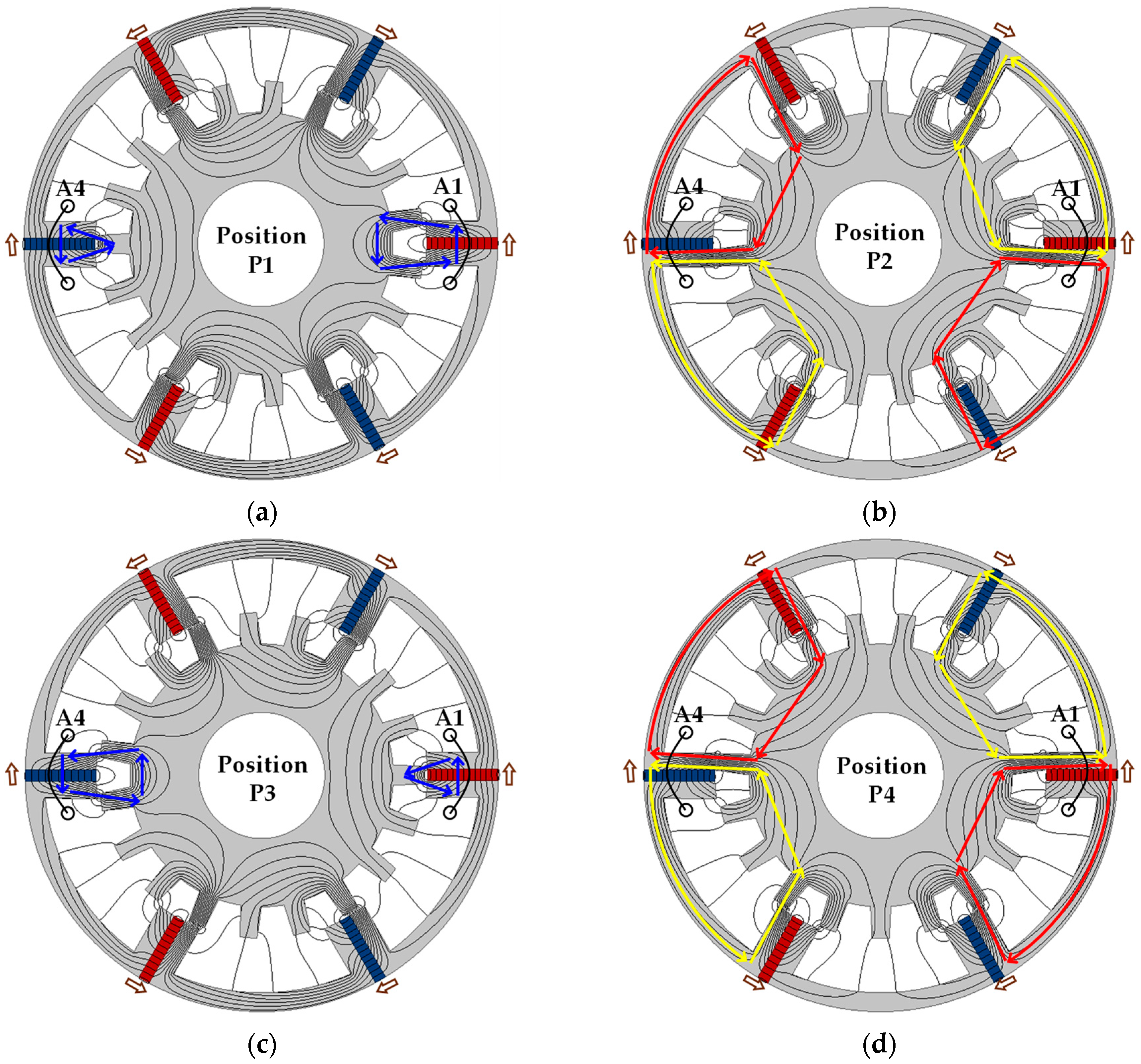
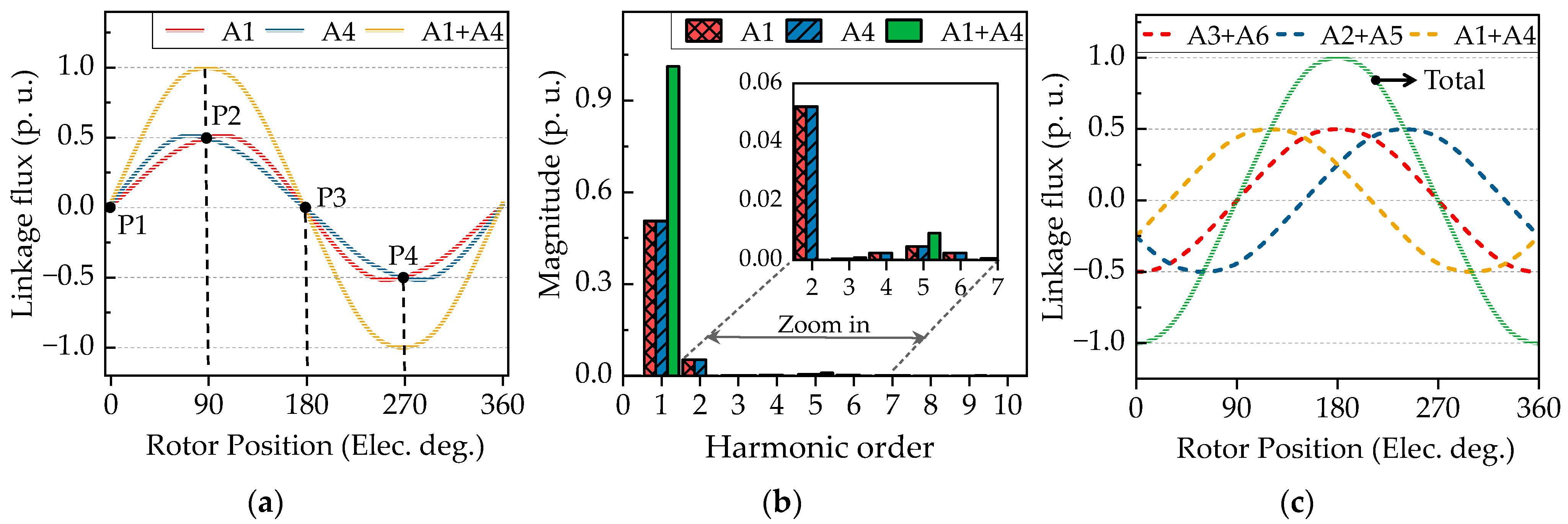
2.2. Working Principle

Figure 2 illustrates the operating principle of the proposed machine through the flux line distribution at four rotor positions, denoted as P1–P4: (P1) ${\theta }_e=0°$, (P2) ${\theta }_e=90°$, (P3) ${\theta }_e=180°$, and (P4) ${\theta }_e=270°$. At positions P1 and P3, the flux passing through coils A1 and A4 is short-circuited, resulting in zero effective flux. In contrast, at positions P2 and P4, the effective flux splits into two symmetric paths, represented by the red and yellow lines, flowing through two adjacent poles. This behavior differs from that of the E-core structure [24], where the flux primarily links only one side of the coil axis and flows dominantly through a fault-tolerant tooth. As the rotor rotates, the linkage flux alternates between maximum and minimum values, known as “flux-switching”.

Figure 3 illustrates the flux waveform of coils A1, A4, and their series-connection A1 + A4. As shown in Figure 3b, although the linkage flux in an individual coil contains significant even harmonics (second, fourth, and sixth harmonics), the flux waveform of the series-connected coils consists exclusively of odd harmonics, resulting in a highly pure sinusoidal flux waveform. This occurs because the even-order harmonics in individual coils have a phase shift of 180°, causing them to cancel each other out when connected in series [25], as confirmed by the Fourier analysis in Figure 3b.

Similarly, the fluxes induced in coil pairs A2 + A5 and A3 + A6 exhibit the same characteristics. Compared to pair A1 + A4, the flux generated by pair A2 + A5 leads by 120° due to its spatial position. Meanwhile, despite the leading spatial position, the flux of pair A3 + A6 lags behind that of A2 + A5 by 60° due to its inverted wound direction. When these three pairs are connected in series, the resulting flux has twice the magnitude of an individual coil pair, as illustrated in Figure 3c. The frequency of this flux varies linearly with rotor speed, generating a voltage at the winding terminal that is also proportional to rotation, making it suitable for speed measurement.

3. Analytical Modeling of Proposed Machine

3.1. Linear Analytical Model

3.1.1. Simplification and Layer Division

To construct a mathematical model for the proposed machine, several assumptions and simplifications are made to ease the analysis [20,21,26].

Since the rotor yoke size is typically designed to avoid saturation, its permeability is assumed to be infinite.

The stator yoke is considered isotropic, with constant magnetic permeability corresponding to the linear region of the $B\left(H\right)$ curve.

In each region, permeability is variable in the tangential direction but constant in the radial direction.

End effects and eddy effects are neglected.

The PMs have uniform magnetization, and their relative permeability is constant.

Mathematically, the machine is divided into five regions in the 2D cylindrical coordinate system illustrated in Figure 4, and the symbols utilized in this section are shown in

Table 1. Nomenclature.

Symbol	Explanation	Symbol	Explanation
$r/\theta /z$	Radius/tangential and axial directions	${\mu }_i^{rt}$	$\mathrm{Permeability} \mathrm{of} \mathrm{the} i$th rotor tooth
$j$	Imaginary unit	${\theta }_r^{ini}$	Initial rotor position
$\overrightarrow{A}$	Magnetic vector potential	$\mathit{A}$	Matrix form of magnetic vector potential
$\overrightarrow{B}$	Magnetic flux density	$\mathit{B}$	Matrix form of magnetic flux density
$\overrightarrow{H}$	Magnetic field strength	$\mathit{H}$	Matrix form of magnetic field strength
$\overrightarrow{J_z}$	Current density vector	${\mathit{M}}_r$	Matrix form of radial component of magnetization
$\mu$	Permeability	${\mathit{M}}_{\theta }$	Matrix form of tangential component of magnetization
${\widehat{\mu }}_n$	CFS coefficient of nth harmonic	${\mathit{A}}^T$	$\mathrm{Transpose} \mathrm{matrix} \mathrm{of} \mathrm{matrix} \mathit{A}$
${\widehat{\mu }}_n^{rec}$	Inverse coefficient of nth harmonic	${\mathit{\mu }}_{c,r}$	Permeability convolution matrix in radial direction
${\mu }_0$	Vacuum permeability	${\mathit{\mu }}_{c,\theta }$	Permeability convolution matrix in tangential direction
${\beta }_{st}$	Span angle of stator teeth	${\mathit{K}}_{\theta }$	$\mathrm{Diagonal} \mathrm{matrix} \mathrm{of} N$
${\beta }_{rt}$	Span angle rotor teeth	$\mathit{G}$	Particular solution of Poisson’s equation
${\beta }_m$	Span angle of PM	${\mathit{W}}^k$	$\mathrm{Eigenvector} \mathrm{matrix} \mathrm{of} \mathrm{matrix} {\left({\mathit{V}}^k\right)}^{0.5}$
$K$	Number of subregions	${\mathit{\lambda }}^k$	$\mathrm{Diagonal} \mathrm{eigenvalue} \mathrm{of} \mathrm{matrix} {\left({\mathit{V}}^k\right)}^{0.5}$
$N$	Highest harmonic order	$k$	Region index
$R_g$	Radius at the middle of airgap	$L_{stk}$	Stack length of the sensor
$T_{cog}$	Cogging torque	${\phi }_{i,j}$	$\mathrm{Flux} \mathrm{passing} \mathrm{through} \mathrm{one} \mathrm{coil} \mathrm{side} \mathrm{in} \mathrm{the} i$$\mathrm{th} \mathrm{slot}, j$th layer
$\psi ,E$	Flux linkage and EMF of the winding	${\psi }_j$	$\mathrm{Total} \mathrm{flux} \mathrm{passing} \mathrm{through} j$th layer
$L$	Winding inductance	$C_i$	$\mathrm{Winding} \mathrm{connecting} \mathrm{matrix} \mathrm{of} j$th layer

. To account for the rectangular shape of the stator teeth and PMs, the stator slot region (III) is divided into multiple subregions. For rotor teeth, discretization of this region is not required because of the short radial length and the absence of PMs. The equivalent dimensions in the simplified geometry are derived from the practical model as follows.

The radius of each subregion is

$$R_j^{III}=R_{is}+\left(j-1\right)\left(R_{sy}-R_{is}\right)/K$$

(3)

where $K$ is the number of subregions.

The arc pole angle corresponding to each subregion can be computed by

$${\beta }_{st,j}^{III}=2\arcsin \left(W_{st}/2/R_j^{III}\right); {\beta }_{m,j}^{III}=2\arcsin \left(W_m/2/R_j^{III}\right)$$

(4)

The other dimensions are given by

$${\beta }_{rt}=2\arcsin \left(W_{rt}/2/R_{or}\right)$$

(5)

$${\beta }_m^{IV}=2\arcsin \left(W_m/2/R_{sy}\right)$$

(6)

3.1.2. Rotor Slot (I), Airgap (II) and External Regions (VI)

The vector potential under matrix form ${\mathit{A}}_z$ satisfies the following Poisson’s equation.

$${\displaystyle \frac{{\mathsf{\partial }}^2{\mathit{A}}_z^k}{\mathsf{\partial }{r}^2}}+{\displaystyle \frac{1}{r}} {\displaystyle \frac{\mathsf{\partial }{\mathit{A}}_z^k}{\mathsf{\partial }r}}-{\displaystyle \frac{1}{r^2}}{{\mathit{V}}^k\mathit{A}}_z^k=0;k=\left(\mathrm{I}\right),\left(\mathrm{I}\mathrm{I}\right),(\mathrm{V})$$

(7)

where ${\mathit{V}}^k={\mathit{\mu }}_{c,\theta }{\mathit{K}}_{\theta }{\mathit{\mu }}_{c,r}^{-1}{\mathit{K}}_{\theta }$, ${\mathit{K}}_{\theta }$ is the diagonal matrix of the greatest harmonic number N. ${\mathit{\mu }}_{c,\theta }$, ${\mathit{\mu }}_{c,r}$ are permeability convolution matrices of Fourier series coefficients (FSCs) in the considered region $k$, given by.

$${\mathit{\mu }}_{c,r}=\left[\begin{array}{ccc}{\widehat{\mu }}_0& \cdots & {\widehat{\mu }}_{-2N}\\ ⋮& \ddots & ⋮\\ {\widehat{\mu }}_{2N}& \cdots & {\widehat{\mu }}_0\end{array}\right]; {\mathit{\mu }}_{c,\theta }=\left[\begin{array}{ccc}{\widehat{\mu }}_0^{rec}& \cdots & {\widehat{\mu }}_{-2N}^{rec}\\ ⋮& \ddots & ⋮\\ {\widehat{\mu }}_{2N}^{rec}& \cdots & {\widehat{\mu }}_0^{rec}\end{array}\right]$$

(8)

where ${\widehat{\mu }}_n^{rec}$ is the inverse coefficient of the $n$th harmonic.

Using the method of separation of variables to solve Equation (7), the general solution is expressed as

$${\mathit{A}}_z^k={{\mathit{W}}^k\left({\displaystyle \frac{r}{R_{outer}^k}}\right)}^{{\mathit{\lambda }}^k}{\mathit{a}}^k+{{\mathit{W}}^k\left({\displaystyle \frac{r}{R_{inner}^k}}\right)}^{-{\mathit{\lambda }}^k }{\mathit{b}}^k; k=(\mathrm{I}),(\mathrm{I}\mathrm{I}),(\mathrm{V})$$

(9)

where $\mathit{a}$, $\mathit{b}$ are unknown coefficients, $R_{outer}^k,R_{inner}^k$ are outer and inner radii of region $k$, ${\mathit{W}}^k$, ${\mathit{\lambda }}^k$ are eigenvector matrix and diagonal eigenvalue of ${\left({\mathit{V}}^k\right)}^{0.5}$.

The convolution matrices for regions (II) and (V) are given by

$${\mathit{\mu }}_{c,\theta }; {\mathit{\mu }}_{c,r}={\mu }_0\mathit{I};$$

(10)

where $\mathit{I}$ is the unit matrix.

From the permeability distribution in Figure 5, FSCs for region (I) are computed by.

$${\widehat{\mu }}_0^I={\displaystyle \frac{1}{2\pi }}\sum _{i=1}^{N_r}{\mu }_0{\beta }_{rl}+{\mu }_i^{rt}{\beta }_{rt}$$

(11)

$${\widehat{\mu }}_n^I={\displaystyle \frac{1}{2\pi jn}}\sum _{i=1}^{N_r}{\mu }_0\left(e^{jn{\gamma }_i^r}-e^{jn\left({\theta }_i^r-{\displaystyle \frac{{\beta }_{rl}}{2}}\right)}\right)+{\mu }_i^{rt}\left(e^{jn\left({\gamma }_i^r+{\beta }_{rt}\right)}-e^{jn{\gamma }_i^r}\right)$$

(12)

where ${\beta }_{rl}=2\pi /N_r-{\beta }_{rt}$, ${\gamma }_i^r={\theta }_i^r+{\beta }_{rl}/2$, ${\theta }_i^r=\left(i-1\right)2\pi /N_r+{\theta }_r^{ini}$, ${\mu }_i^{rt}$ is the permeability of the $i$th rotor tooth, and ${\theta }_r^{ini}$ is the initial rotor position.

3.1.3. Stator Slot and Stator Yoke Regions (III), (IV)

The magnetic vector potential ${\mathit{A}}_z$ satisfies the following Poisson’s equation.

$${\displaystyle \frac{{\mathsf{\partial }}^2{\mathit{A}}_z^k}{\mathsf{\partial }{r}^2}}+{\displaystyle \frac{1}{r}} {\displaystyle \frac{\mathsf{\partial }{\mathit{A}}_z^k}{\mathsf{\partial }r}}-{\displaystyle \frac{1}{r^2}}{{\mathit{V}}^k\mathit{A}}_z^k=-{\displaystyle \frac{{\mu }_0}{r}}\left(j{\mathit{U}}^k{\mathit{M}}_r^k+{\mathit{M}}_{\theta }^k\right);k=\left(\mathrm{I}\mathrm{I}\mathrm{I}\right),\left(\mathrm{I}\mathrm{V}\right)$$

(13)

where ${\mathit{U}}^k={\mathit{\mu }}_{c,\theta }{\mathit{K}}_{\theta }{\mathit{\mu }}_{c,r}^{-1}$. The general solution of (13) is given by

$${\mathit{A}}_z^k={{\mathit{W}}^k\left({\displaystyle \frac{r}{R_{outer}^k}}\right)}^{{\mathit{\lambda }}^k}{\mathit{a}}^k+{{\mathit{W}}^k\left({\displaystyle \frac{r}{R_{inner}^k}}\right)}^{-{\mathit{\lambda }}^k }{\mathit{b}}^k+r{\mathit{G}}^k; k=(\mathrm{I}\mathrm{I}\mathrm{I}),(\mathrm{I}\mathrm{V})$$

(14)

where ${\mathit{G}}^k$ is the particular solution of (13), defined by

$${\mathit{G}}^{\mathit{k}}=j{\mu }_0{\left[{\mathit{V}}^k-\mathit{I}\right]}^{-1}{\mathit{U}}^k{\mathit{M}}_r^k+{\mu }_0{\left[{\mathit{V}}^k-\mathit{I}\right]}^{-1}{\mathit{M}}_{\theta }^k$$

(15)

where ${\mathit{M}}_r^k$ and ${\mathit{M}}_{\theta }^k$ are the magnetization matrices of radial and tangential components of the magnetization vector $M$.

$${\mathit{M}}_r^k=\left[{\widehat{M}}_{r,-N}^k\dots {\widehat{M}}_{r,N}^k\right];{\mathit{M}}_{\theta }^k=\left[{\widehat{M}}_{\theta ,-N}^k\dots {\widehat{M}}_{\theta ,N}^k\right];k=\left(\mathrm{I}\mathrm{I}\mathrm{I}\right),\left(\mathrm{I}\mathrm{V}\right)$$

(16)

$${\widehat{M}}_{\theta ,n}^k={\displaystyle \frac{1}{2\pi jn}}\sum _{i=1}^{N_s}{\displaystyle \frac{B_r{\left(-1\right)}^{i+1}}{{\mu }_0}}{e}^{jn\left({\theta }_i^k+{\displaystyle \frac{{\beta }_{sl}^k}{2}}+{\beta }_{st}^k\right)}\left(e^{jn{\beta }_m^k}-1\right); {\widehat{M}}_{r,n}^k=0$$

(17)

From the permeability distribution shown in Figure 5, FSCs for subregion $j$ in Region (III) are derived from

$${\widehat{\mu }}_0^j={\displaystyle \frac{1}{2\pi }}\sum _{i=1}^{N_s}{\mu }_0{\beta }_{sl,j}^{III}+{\mu }_m{\beta }_{m,j}^{III}+\left({\mu }_{i,j}^{lst}+{\mu }_{i,j}^{rst}\right){\beta }_{st,j}^{III}; {\widehat{\mu }}_n^{III,j}={\displaystyle \frac{1}{2\pi jn}}\sum _{i=1}^{N_s}{P}_i^j+Q_i^j$$

(18)

$$P_i^j={\mu }_0\left(e^{jn{\gamma }_i^j}-e^{jn\left({\theta }_i^j-{\displaystyle \frac{{\beta }_{sl}^j}{2}}\right)}\right)+{\mu }_m\left(e^{jn\left({\tau }_i^j+{\beta }_m^j\right)}-e^{jn{\tau }_i^j}\right)$$

(19)

$$Q_i^j={\mu }_{i,j}^{lst}\left(e^{jn{\tau }_i^j}-e^{jn{\gamma }_i^j}\right)+{\mu }_{i,j}^{rst}\left(e^{jn\left({\tau }_i^j+{\beta }_{m,j}^{III}+{\beta }_{st,j}^{III}\right)}-e^{jn\left({\tau }_i^j+{\beta }_{m,j}^{III}\right)}\right)$$

(20)

where ${\gamma }_i^j={\theta }_i^s+{\beta }_{sl,j}^{III}/2$, ${\tau }_i^j={\theta }_i^s+{\beta }_{sl,j}^{III}/2+{\beta }_{st,j}^{III}$, and ${\theta }_i^s=\left(i-1\right)2\pi /N_s$. ${\mu }_{i,j}^{lst}$ and ${\mu }_{i,j}^{rst}$ are the permeability values of the iron parts at the left- and right-hand side of a magnet.

For Region IV, because the saturation is focused on the parts closing to the airgap, such as teeth [27,28], the stator yoke is usually in the linear range of $B\left(H\right)$ curve. A finite permeability value, such as ${\mu }_{sy}=3000$, can be set for all iron parts in this region. The FSCs for the convolution matrices in this region are derived by

$${\widehat{\mu }}_0^{IV}={\displaystyle \frac{1}{2\pi N_s}}\left({\mu }_m{\beta }_m^{IV}+{\mu }_{sy}\left({\displaystyle \frac{2\pi }{N_s}}-{\beta }_m^{IV}\right)\right)$$

(21)

$${\widehat{\mu }}_n^{IV}={\displaystyle \frac{1}{2\pi jn}}\sum _{i=1}^{N_r}{\mu }_m\left(e^{jn\left({\gamma }_i^{IV}+{\beta }_m^{IV}\right)}-e^{jn{\gamma }_i^{IV}}\right)+{\mu }_{sy}\left(e^{jn{\gamma }_i^{IV}}-e^{jn\left({\tau }_i^{IV}+{\displaystyle \frac{{\beta }_m^{IV}}{2}}\right)}\right)$$

(22)

where ${\gamma }_i^{IV}={\theta }_i^s+\pi /N_s-{\beta }_m^{IV}/2$, ${\tau }_i^{IV}={\theta }_i^s-\pi /N_s$.

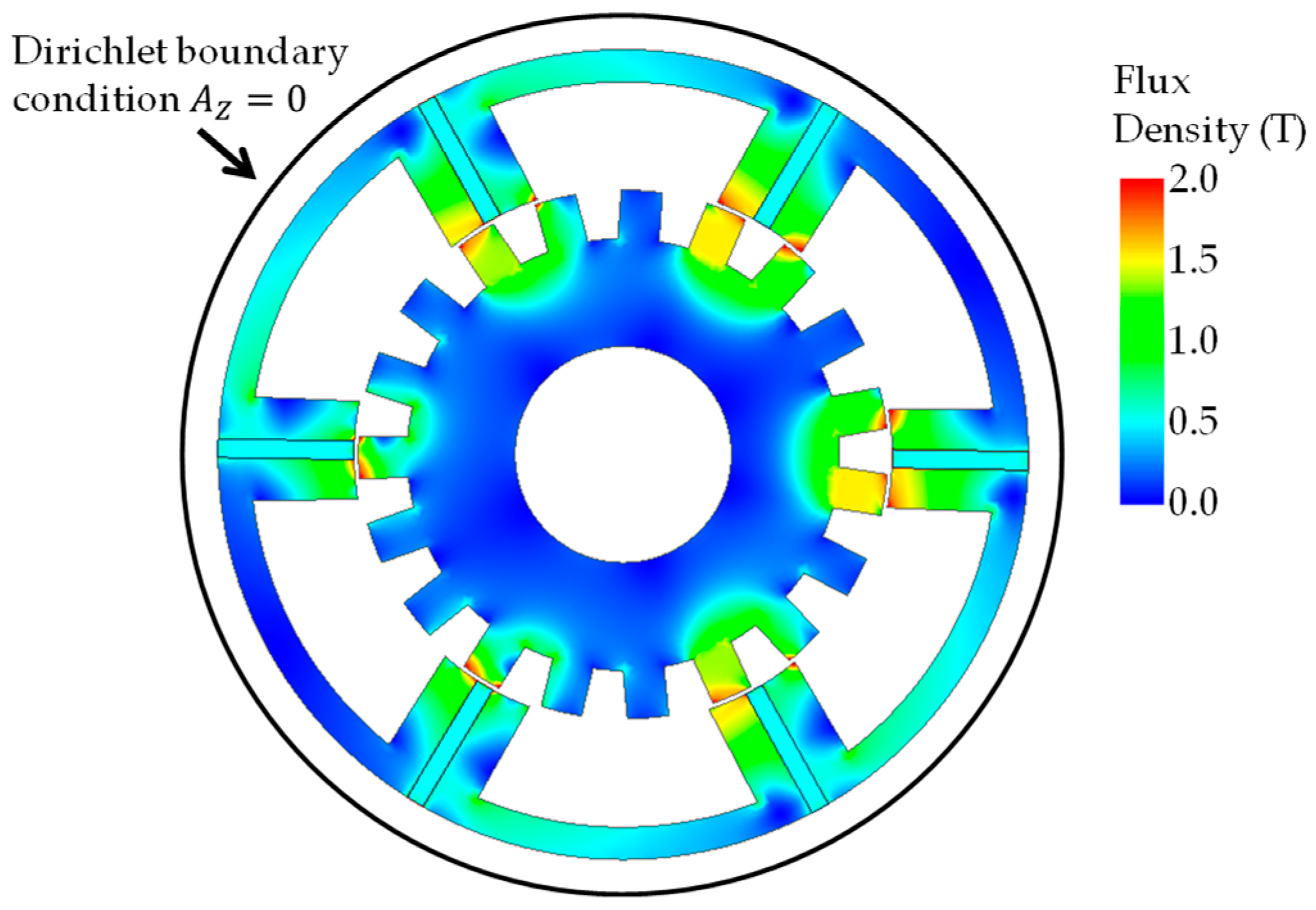
3.1.4. Boundary Conditions (BCs)

The BCs of the continuity of magnetic vector potential and magnetic field strength are applied to interfaces at $R_{or}$, $R_j^{III}$, $R_{sy}$, and $R_{os}$. Additionally, at $R_{ir}$, the Neumann condition is employed due to the assumption of infinite permeability, and at $R_{ext}$ the Dirichlet condition is used. $R_{ext}$ is assumed to be a considerable distance where the magnetic field is negligible compared to the machine field. The resulting boundary conditions are expressed as follows.

$${\mathit{H}}_{\theta }^I{|}_{r=R_{ir}}=0; {\mathit{A}}_z^V{|}_{r=R_{ext}}=0$$

(23)

$${\mathit{A}}_z^I{|}_{r=R_{or}}-{\mathit{A}}_z^{II}{|}_{r=R_{or}}=0; {\mathit{H}}_z^I{|}_{r=R_{or}}-{\mathit{H}}_z^{II}{|}_{r=R_{or}}=0$$

(24)

$${\mathit{A}}_z^{II}{|}_{r=R_{is}}-{\mathit{A}}_z^{III,1}{|}_{r=R_{is}}=0; {\mathit{H}}_z^{II}{|}_{r=R_{is}}-{\mathit{H}}_z^{III,1}{|}_{r=R_{is}}=0$$

(25)

$${\mathit{A}}_z^{III,j}{|}_{r=R_{j+1}^{III}}-{\mathit{A}}_z^{III,j+1}{|}_{r=R_{j+1}^{III}}=0; {\mathit{H}}_z^{III,j}{|}_{r=R_{j+1}^{III}}-{\mathit{H}}_z^{III,j+1}{|}_{r=R_{j+1}^{III}}=0$$

(26)

$${\mathit{A}}_z^{III,j}{|}_{r=R_{sy}}-{\mathit{A}}_z^{IV}{|}_{r=R_{sy}}=0; {\mathit{H}}_z^{III,j}{|}_{r=R_{sy}}-{\mathit{H}}_z^{IV}{|}_{r=R_{sy}}=0$$

(27)

$${\mathit{A}}_z^{IV}{|}_{r=R_{os}}-{\mathit{A}}_z^V{|}_{r=R_{os}}=0; {\mathit{H}}_z^{IV}{|}_{r=R_{os}}-{\mathit{H}}_z^V{|}_{r=R_{os}}=0$$

(28)

Finally, the unknown coefficients in (9) and (14) are determined by solving the system of (23)–(28).

3.1.5. Nonlinear Solution Derivation

After constructing a linear model with permeability as an input, the flux density obtained in the stator and rotor teeth is used to update the permeability of these iron parts based on the $B\left(H\right)$ curve of the material. This iterative process is applied using the relaxation method to find the converged solution of the magnetic field. The detailed iterative process has been thoroughly presented in [20,21] and therefore is not repeated in this paper. The magnetic material used for the core is 35PN440 steel, with the characteristic curves illustrated in Figure 6.

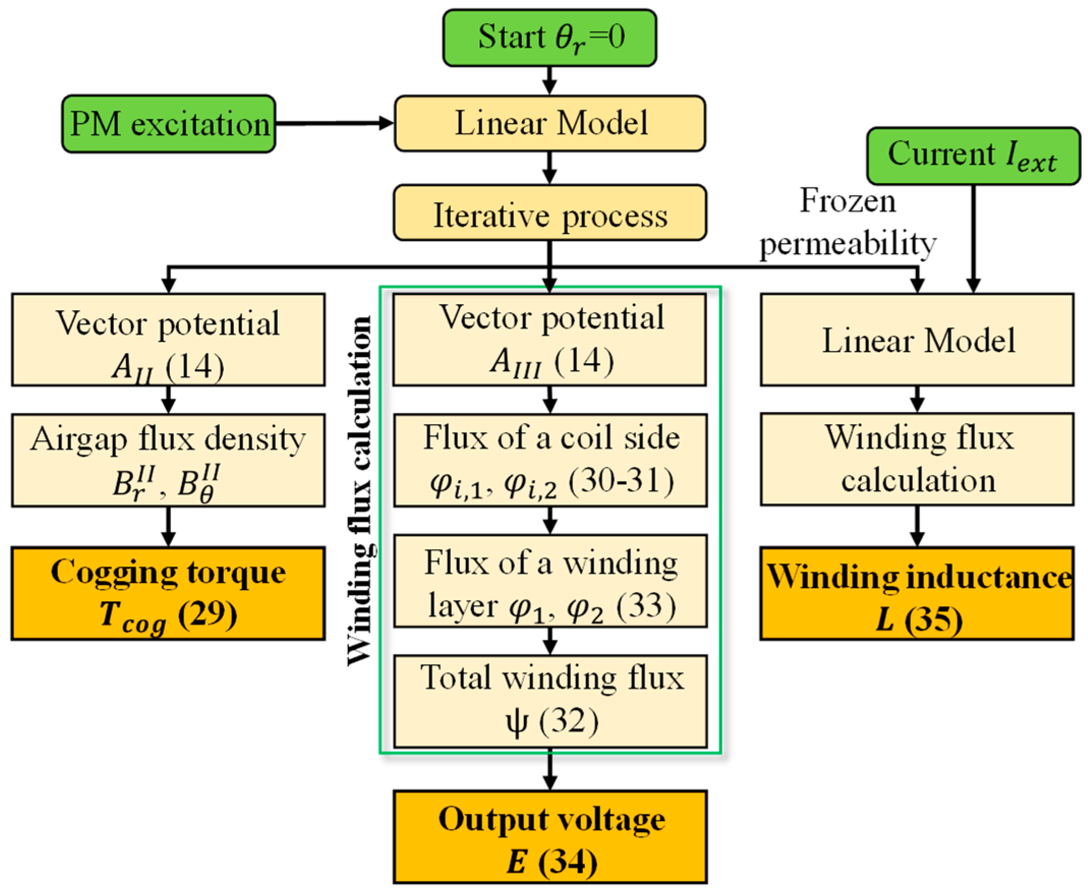
3.2. Performance Derivation

The proposed analytical model calculates several performance criteria, including cogging torque, output voltage, and winding inductance, which are calculated using Equations (29)–(35). For clarity, the overall computation process is illustrated in the flowchart shown in Figure 7.

The cogging torque is computed by

$$T_{cog}={\displaystyle \frac{l_{stk}{R}_g^2}{{\mu }_0}}{\int }_0^{2\pi }{B}_{\theta }^{II}\left(R_g,\theta \right)B_r^{II}\left(R_g, \theta \right)d\theta$$

(29)

The output voltage can be deducted as follows.

First, the flux passing through one coil side in the $i$th slot is expressed as

$${\phi }_{i,1}^{III,j}={\displaystyle \frac{L_{stk}}{A_{slot}^{III,j}}}{\int }_{{\theta }_i^s-{\displaystyle \frac{{\beta }_{sl}^k}{2}}}^{{\theta }_i^s}{\int }_{R_{inner}}^{R_{outer}}{A}_z^{III,j}(\theta ,r)rdrd\theta$$

(30)

$${\phi }_{i,2}^{III,j}={\displaystyle \frac{L_{stk}}{A_{slot}^{III,j}}}{\int }_{{\theta }_i^s}^{{\theta }_i^s+{\displaystyle \frac{{\beta }_{sl}^k}{2}}}{\int }_{R_{inner}}^{R_{outer}}{A}_z^{III,j}(\theta ,r)rdrd\theta$$

(31)

where $A_{slot}^{III,j}$ is the slot area in the $j$th subregion and $L_{stk}$ is the stack length.

The total flux passing through the winding is written as

$$\psi =\sum _{k=1\to j}{N}_t\left({\phi }_1^{III,j}+{\phi }_2^{III,j}\right)$$

(32)

where $N_t$ is the number of turns per coil.

$${\phi }_1^{III,j}=C_1{\left[{\phi }_{i,1}^{III,j},\dots ,{\phi }_{N_s,1}^{III,j}\right]}^T; {\phi }_2^{III,j}=C_2{\left[{\phi }_{i,2}^{III,j},\dots ,{\phi }_{N_s,2}^{III,j}\right]}^T$$

(33)

$$C_1=\left[\begin{array}{cc}\begin{array}{ccc}-1& 1& -1\end{array}& \begin{array}{ccc}-1& 1& -1\end{array}\end{array}\right]; C_2=\left[\begin{array}{cc}\begin{array}{ccc}1& 1& -1\end{array}& \begin{array}{ccc}1& 1& -1\end{array}\end{array}\right]$$

Then the output voltage of the winding is derived as

$$E=-d\psi /dt$$

(34)

After nonlinear solutions are found, the PM excitation is extruded and replaced by a small current $I$, the obtained linkage flux is used to calculate the winding inductance as

$$L={\psi }_I/I$$

(35)

4. FEA Verification

To demonstrate the accuracy of the proposed model and investigate the effects of the stator teeth layer number, three cases corresponding to one, two, and three layers are analyzed in this section. In each case, the results from analytical models are compared with those from a 2D finite element (FE) model in Ansys Maxwell. Since the proposed sensor operates under permanent magnet excitation, no external current source is applied to the windings. The simulation domain includes the stator, rotor, air gap, and external space with the Dirichlet boundary condition ($A_z=0$) applied to the outer boundary of the problem space. The rotor is assigned a mechanical rotational speed, and transient simulation is used to observe the induced voltage waveform, flux density distribution, and other field quantities over time. The main parameters of the benchmark model are detailed in

Table 2. Initial design parameters.

Parameter	Symbol	Value
Stack length (mm)	$L_{stk}$	43.0
Outer/inner stator radius (mm)	$R_{os}$	37.5/24.9
Outer/inner rotor radius (mm)	$R_{or}$	24.4/20.0
Stator/Rotor teeth width (mm)	$W_{rt}$	3.70/3.85
PM width (mm)	$W_{PM}$	1.75
Stator yoke thickness (mm)	$H_{ys}$	3.0
PM remanence (T)	$B_r$	1.28
Number of turns per coil	$N_t$	63

, where the outer stator diameter and stack length are selected based on a commercial AC tachogenerator [29]. Figure 8 illustrates the flux density distribution of the FE model under PM excitation. The results show that mild saturation occurs at the stator and rotor teeth, reaching approximately 1.6 T. In contrast, the highest flux density in the yoke is around 1.0 T, significantly lower than that in the teeth and well below the saturation threshold. This supports the assumption of infinite permeability made in Section 3.1.1.

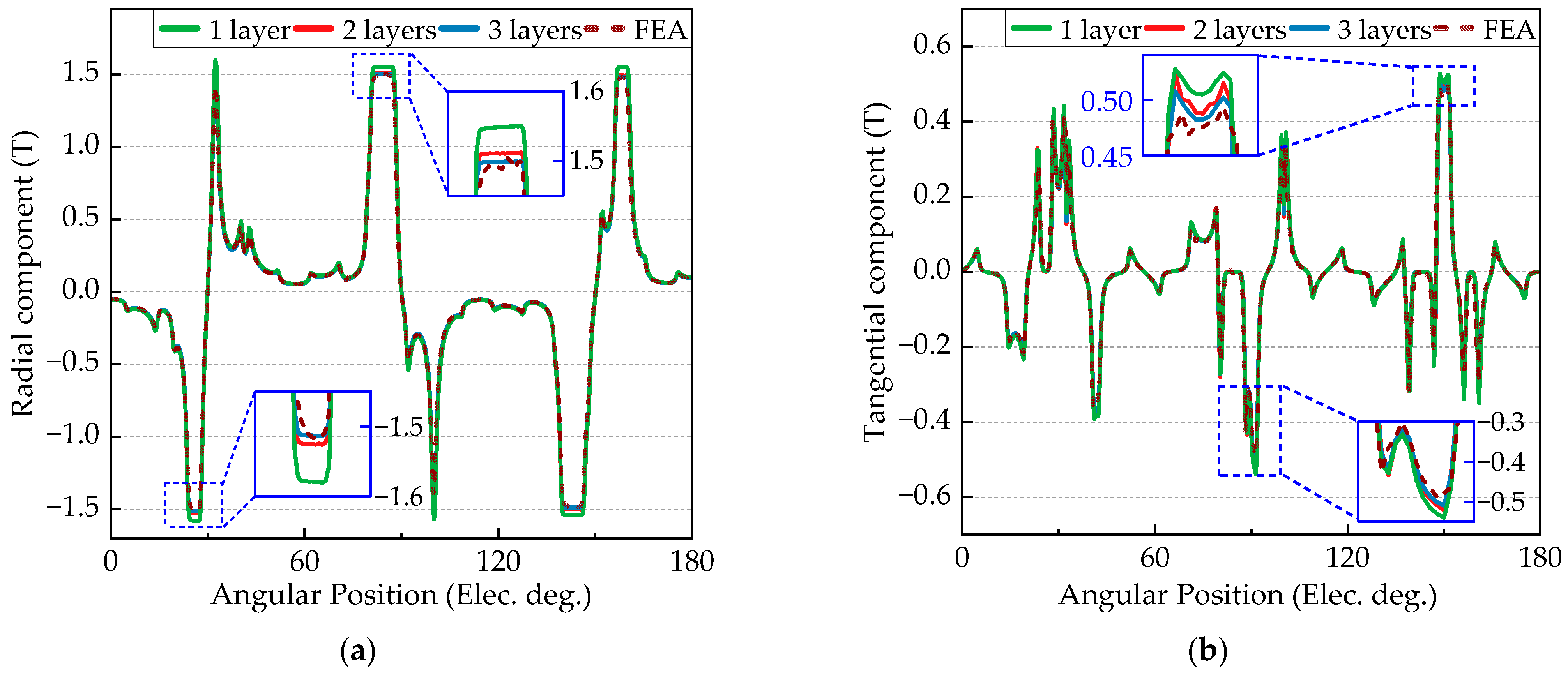
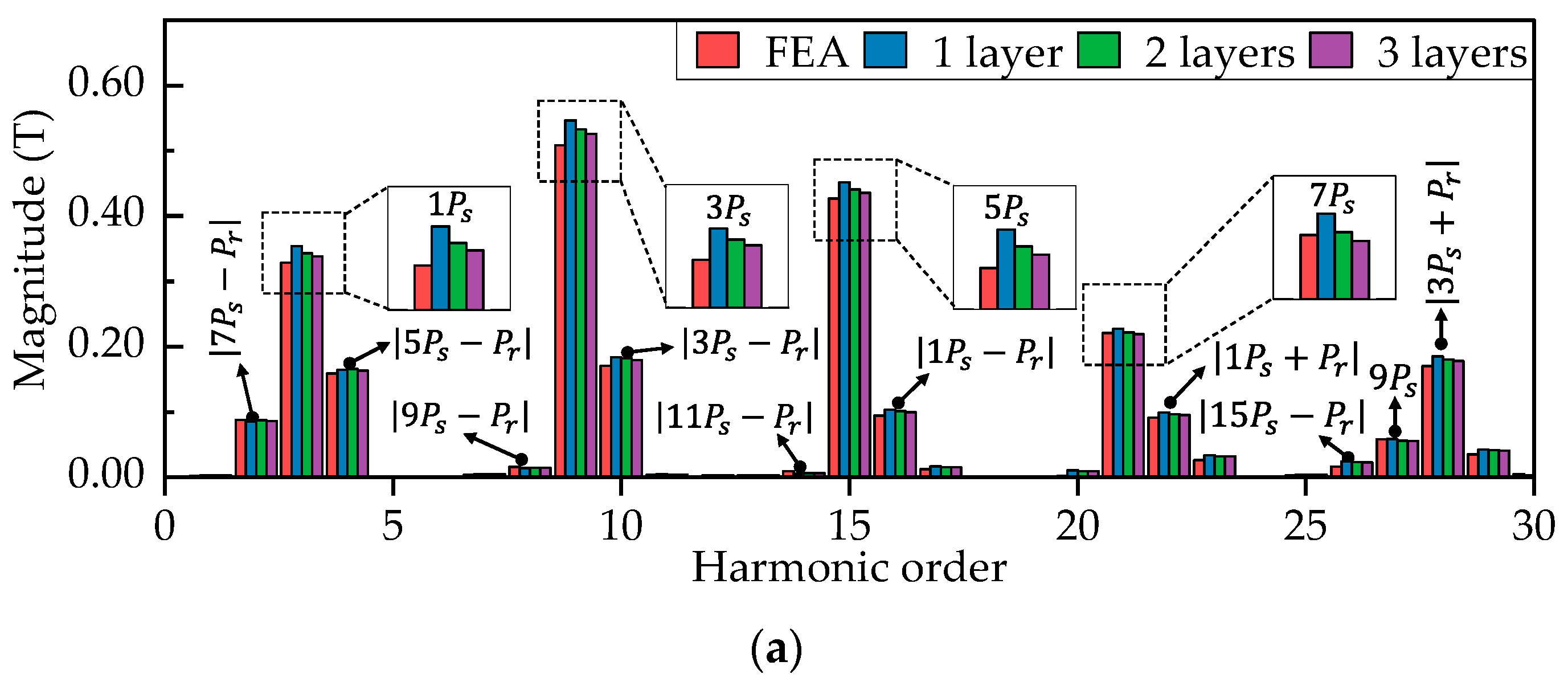
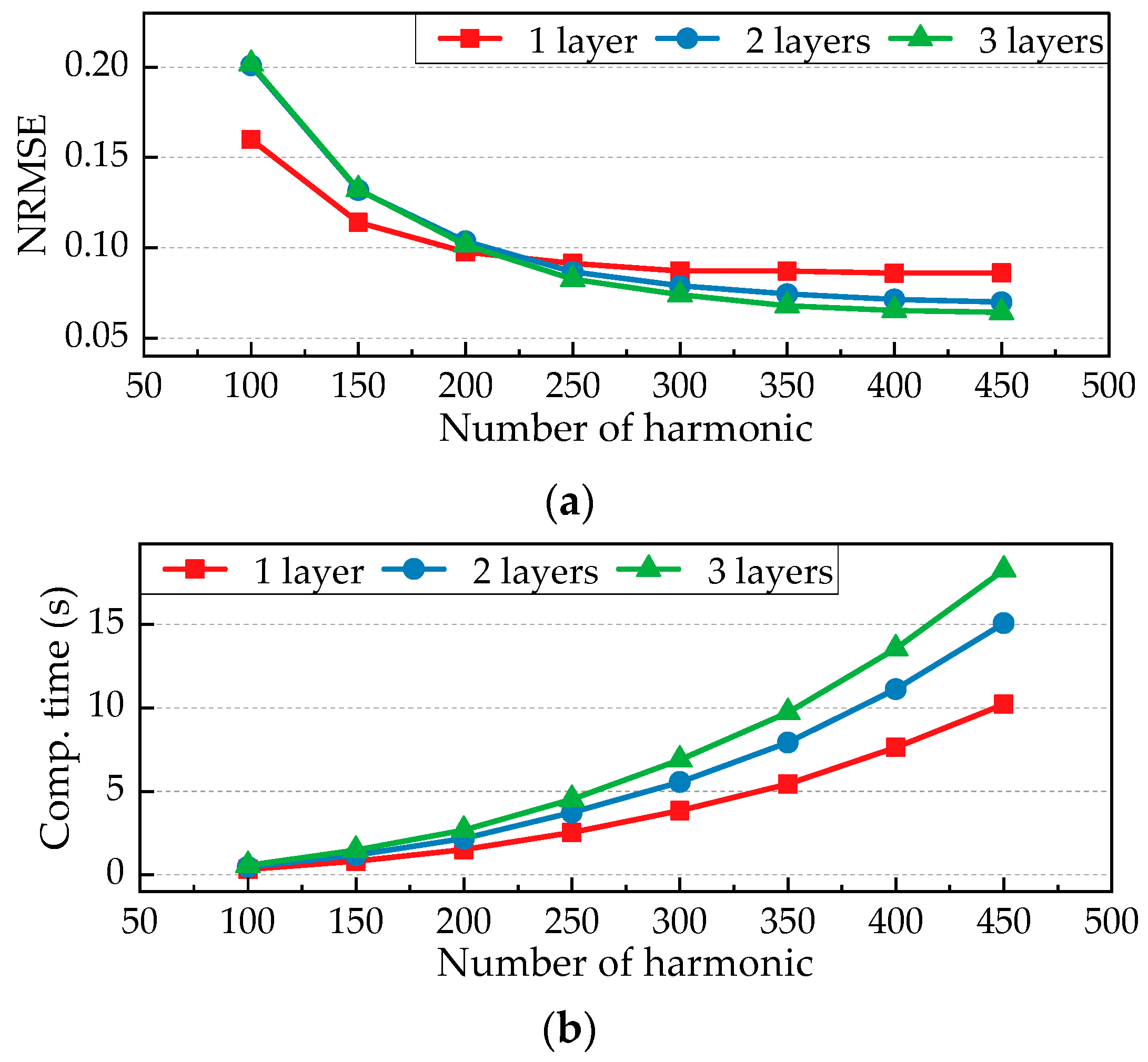
4.1. Magnetic Field Analysis

Figure 9 shows the magnetic field distributions (MFD) at the airgap, obtained from analytical and FE models, in radial and tangential directions, respectively. Overall, all three cases agree acceptably with the FE model. However, the accuracy of the analytical results improves as the number of stator teeth layers increases. Specifically, the largest deviations occur when only one stator teeth layer is used, as this configuration introduces the most significant differences in the PM area. Whereas, with three layers, the analytical model more accurately approximates the geometry of the stator teeth and the PMs, resulting in excellent consistency between the analytical and FE models.

Furthermore, the Fast Fourier Transform (FFT) analysis of the MFD is illustrated in Figure 10. Unlike conventional machine types such as surface-mounted permanent magnet (SPM) or interior permanent magnet (IPM) machines, the air-gap flux of FSPMM contains various harmonics due to the flux modulation effect [30,31]. First, the dominant harmonics are the odd multiples of the stator pole pair number (PPN), or PPN of PMs, $P_s$, which is determined by

$$P_s=N_s/2$$

(36)

The PPN of armature winding is defined by.

$$P_w=\left|P_r-P_s\right|$$

(37)

Meanwhile, multiple working harmonics exist in the air gap flux. These harmonics contribute to EMF generation by ensuring that the PPN of the magnetic field excited by the PMs under rotor modulation, denoted as $P_{i,j}^s$, matches that of the magnetic field excited by the armature winding, denoted as $P_{m,k}^w$, and that both fields rotate at the same speed [32].

$$P_{i,j}^s=\left|i{P}_s\pm j{P}_r\right|;P_{m,k}^w=\left|m{P}_w\pm k{P}_r\right|$$

(38)

where $P_r=N_r$, $i,m=\mathrm{1,3},5,\dots ,\mathrm{\infty }$, and $j,k=\mathrm{0,1},2,\dots ,\mathrm{\infty }$;

FFT analysis reveals the same trend: as the number of layers increases, the AM results become closer to those obtained from the FE model. Notably, while the single-layer case exhibits the largest deviation from the FE results, the two-layer model significantly improves accuracy and shows only a minor difference compared to the three-layer case.

To further evaluate the effects of the layer number on the AM, the computation time and normalized root mean square of error (NRMSE) [33] of the MFD for each case are recorded as a function of the number of harmonics, as illustrated in Figure 11. The accuracy of the proposed model is estimated by

$$\mathrm{N}\mathrm{R}\mathrm{M}\mathrm{S}\mathrm{E}=\sqrt{{\displaystyle \frac{\sum {\left[B_{ana}\left(i\right)-B_{FE}\left(i\right)\right]}^2}{\sum B_{FE}{\left(i\right)}^2}}}$$

(39)

where $B_{ana}\left(i\right)$ and $B_{FE}\left(i\right)$ are values of the $i$th estimation of magnetic flux density obtained by analytical and FE models, respectively.

The results indicate that the NRMSE of all cases begins to converge around $N=250$, with the deviation between the two-layer and three-layer cases being smaller than that between the one-layer and two-layer cases. Regarding computation time, it exhibits a direct proportionality to the number of harmonics, as an increase in harmonics leads to a larger matrix size in the Equation system (23)–(28). Moreover, in terms of computational efficiency, the two-layer case offers a significant reduction in computation time compared to the three-layer counterpart while maintaining high accuracy. Although the one-layer case has the shortest computation time, its NRMSE converges at a much higher value than the other cases, resulting in a notable loss of accuracy.

As a result, the two-layer solution presents the best trade-off between accuracy and computational efficiency. Therefore, this configuration is adopted for the subsequent analyses in this paper.

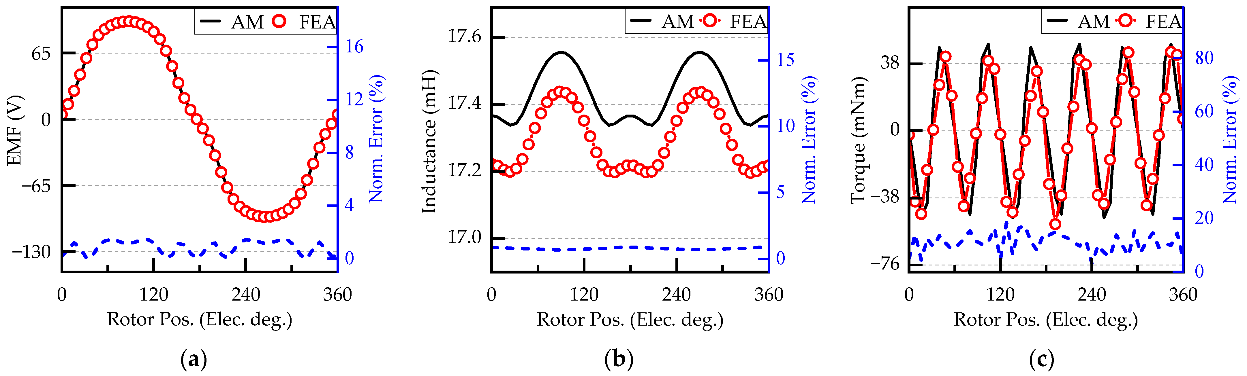
4.2. Performance Comparison

At a rotational speed of 1500 rpm, the EMF in the stator winding is illustrated in Figure 12a. Meanwhile, the stator winding inductance and cogging torque waveforms are shown in Figure 12b,c, respectively. It is observed that the EMF waveforms derived from both the AM and FEA show excellent agreement. A slight discrepancy is noted in the stator winding inductance, where the FEA result (17.32 mH) is lower than the AM prediction (17.49 mH), yielding a deviation of 0.81%.

Regarding cogging torque, a slight difference between the two models is observed. This deviation is primarily attributed to higher-order harmonics in the airgap flux, in which the AM is inherently limited due to its finite harmonic order N. Nevertheless, the AM still provides accurate and reliable predictions, making it suitable for further evaluations and design optimizations.

5. Parametric Optimization

In this section, the proposed AM is used to conduct parametric analyses and optimize the shape of the machine. Generally, the output voltage should be maximized while minimizing the cogging torque and winding inductance. A small cogging torque reduces machine vibration, while lower winding inductance leads to a smaller voltage drop in the winding when the output is connected to a load. Furthermore, the output voltage waveform is optimized to be as sinusoidal as possible, reducing noise by decreasing the total harmonic distortion (THD).

The initial machine parameters are listed in Table 2, where the split ratio $R_{is}/R_{os}$, the rotor teeth width $W_{rt}$, stator teeth width $W_{st}$, and PM width $W_{PM}$ are considered as the optimal variables. The optimal objectives include cogging torque, the magnitude of the first-order EMF, THD, and winding inductance. Refs. [16,27,34] show that the combinations of stator teeth, rotor teeth, and PM widths are more sensitive to the performance of FSPM machines. Therefore, the optimization of the proposed machine follows this procedure: first, the ratio $k_{rm}=W_{rt}/W_{PM}$ and split ratio are selected according to the four optimal objectives at a specific ratio of $k_{rs}=W_{rt}/W_{st}$. This process is repeated at different $k_{rs}$ ratios to determine the optimized machine geometry.

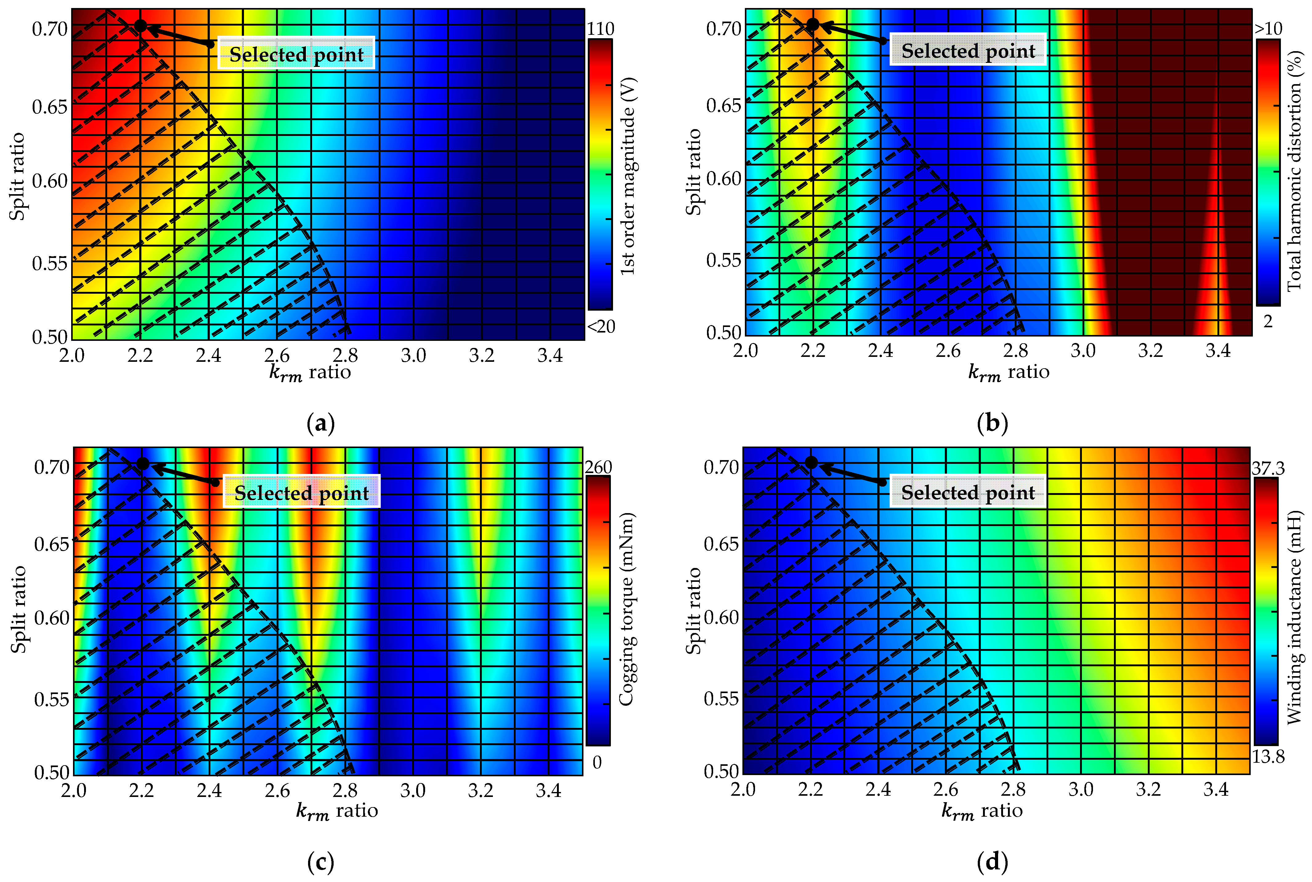
5.1. Split Ratio and Rotor Teeth Ratio

In this part, the two coefficients of split ratio and $k_{rm}$ ratio are considered as variables. Herein, the split ratio is changed by fixing the outer stator radius while the $k_{rm}$ is adjusted by changing the rotor teeth width $W_{rt}$. The $k_{rs}$ is set to 1.

First, the maximum teeth flux density limitation is chosen under saturation point 1.6 T of the materials. This value should be limited to minimize core losses and ensure computation efficiency. When the machine is more saturated, additional harmonics at the airgap are produced, which the analytical model cannot capture, causing a greater error in cogging torque prediction.

The maximum flux density on stator/rotor teeth is depicted in Figure 13, where the saturated range occurs mainly for small $k_{rm}$ and split ratios. When the split ratio gets smaller, the radial length of PM increases, producing more flux. As a result, a small tooth is insufficient for flux flow.

Figure 14 shows the variations of the 1st-order EMF, THD, cogging torque, and winding inductance, where the EMF and inductance improve with a greater split ratio and smaller $k_{rm}$. Cogging torque and THD are inversely proportional to the split ratio. Based on the feasible region, an optimal point is chosen at $k_{rm}=2.2$ and split ratio = 0.7, with 1st EMF = 98.3 V, THD = 8.14%, cogging torque = 32.4 mNm and inductance = 15.3 mH.

5.2. Stator and Rotor Teeth Width

The process in Section 4.1 is repeated in this part but with a different stator and rotor teeth ratio $k_{rs}={\beta }_{rt}/{\beta }_{st}$. Specifically, with a rotor teeth width ${\beta }_{rt}=k_{rm}{\beta }_m$, the stator teeth width is determined by ${\beta }_{st}=k_{rs}{\beta }_{rt}$. For each $k_{rs}$ value, an optimal solution is selected based on the optimal objectives, as illustrated in Figure 14. With the range of $k_{rs}=0.9$ to $1.4$, the obtained solutions are shown in Figure 15. From the results, a final solution is chosen with $k_{rs}=1.2$, $k_{rt}=2.1$, and split ratio $=0.7$ with the characteristics: 1st EMF = 111.6 V, THD = 3.3%, cogging torque = 61.4 mNm, and winding inductance = 12.95 mH. Although the cogging torque is higher than the case $k_{rs}=1$, the three remaining aspects have improved much. Using FEA to validate the final design, the obtained results are 1st EMF = 110.5 V, THD = 1.53%, cogging torque = 78.4 mNm, and winding inductance = 12.78 mH, demonstrating the effectiveness of the optimization.

6. Performance of Optimal Design

Because the analytical model cannot capture the eddy current effects of the PM on the stator, a FE coupling model between Ansys Maxwell 2D and Twinbuilder is built to extract the performance of the proposed speed sensor. Additionally, considering the low power of the speed sensor, the AWG (American wire gauge) 34 conductor with a 0.16 mm diameter is selected for the stator winding. Due to the small size of the conductor, the additional length of one turn caused by the end-winding height can be neglected. The stator resistance is determined by

$$R_{wind}={\rho }_{co}{L}_{wind}/S_{cond}$$

(40)

$$L_{wind}=N_s{N}_t\left[2\left(L_{stk}+2W_{st}+W_{PM}\right)\right]$$

(41)

where ${\rho }_{co}$ is the copper resistivity, and $L_{wind}$ is the total length of the winding. With the chosen conductor size and the design dimensions, the stator winding resistance is 40.25 Ω.

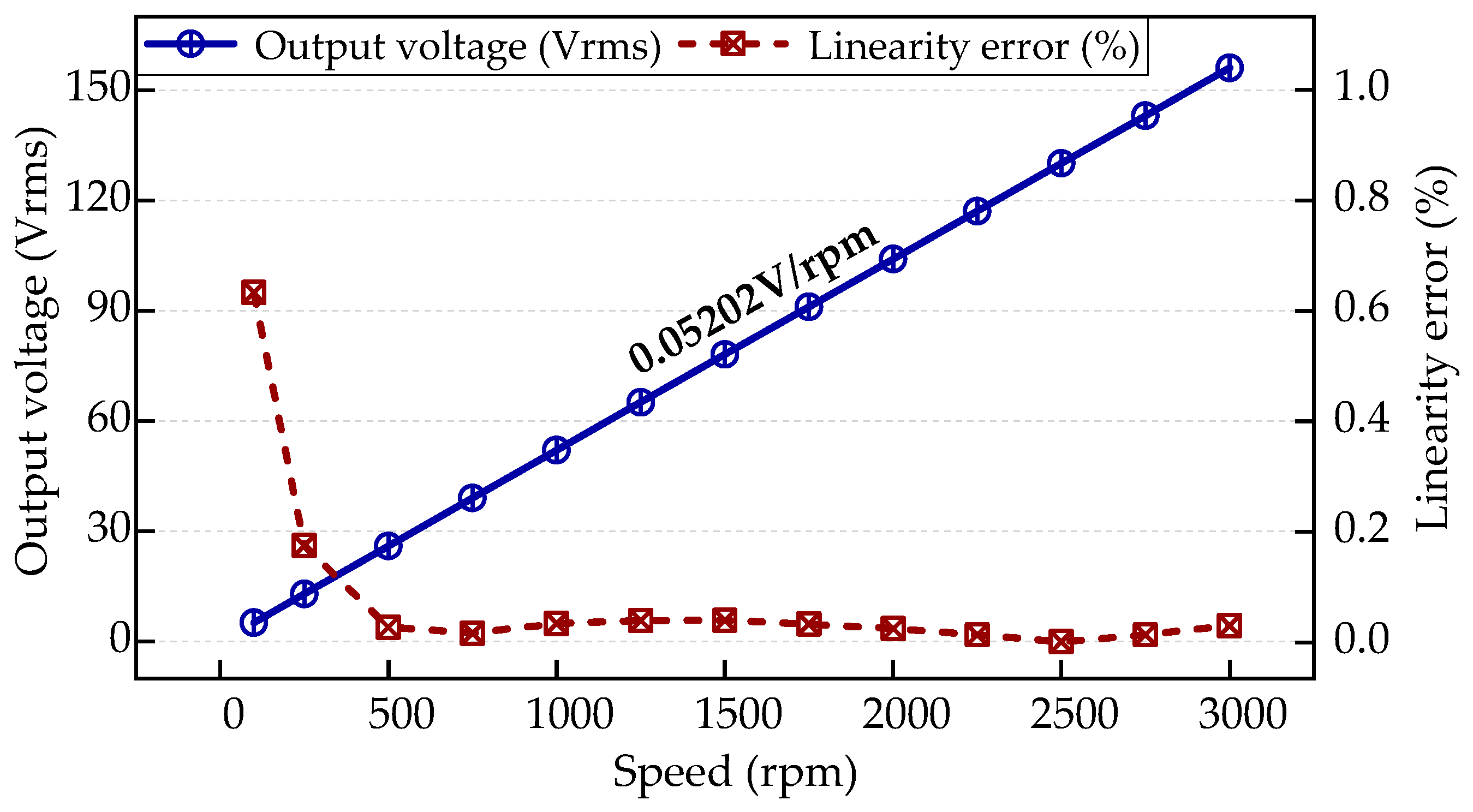
6.1. Voltage Characteristics (Constant Load Characteristics)

Figure 16 shows the output voltage characteristics against the speed from 100 rpm to 3000 rpm under a constant load of 1 mA. It is evident that the proposed design exhibits brilliant linearity and output voltage, with the output ranging from 5.16 to 156.0 Vrms. The maximum error recorded is 0.63% at 100 rpm. Compared to the product [29], the output voltage is 31.5% higher, while the maximum linearity error is smaller than that of the commercial product by 1%. It is noted that a higher voltage drop at stator resistance causes a higher deviation at low speeds. Compared to the design in [8], although the sensor volume is approximately three times larger, the proposed design achieves over 3000 times higher output sensitivity without requiring any external excitation source. Additionally, the linearity performance is comparable, with a maximum linearity error of 0.63% in the proposed model versus 0.67% in [8].

6.2. Varying Load Characteristics

Figure 17 shows the voltage drop of the proposed design according to the speed and load under two cases of load resistance: 2500 Ω and 5000 Ω. At the heavier load, the load current increases from 5 mA to 60 mA, and the voltage drop changes from 1.28% to 1.68%. Specifically, at 1500 rpm and 30 mA, the voltage drop is 1.58%, compared to 2.5% for the product [29], and this ratio changes negligibly despite the higher load current. At the lighter load, the voltage drop is much lower than at the first load across the speed range, with a maximum of 0.83%. These characteristics of the proposed design are comparable to commercial products.

7. Conclusions

This paper introduced a flux-switching-based speed sensor with a 6-stator-slot/19-rotor-pole (6s/19p) topology to provide a high-performance, cost-effective alternative to conventional speed measurement technologies. By leveraging the flux-switching principle, the proposed design achieves higher output voltage, improved linearity, and reduced permanent magnet (PM) consumption. To accurately model the sensor’s electromagnetic behavior, a nonlinear analytical model (NAM) based on harmonic modeling (HM) was developed. This model effectively accounts for core saturation effects and the rectangular geometry of PMs and stator teeth, ensuring better agreement with finite element analysis (FEA) results. Among the analytical models tested, the two-layer model was identified as the best trade-off between computational efficiency and accuracy, demonstrating high fidelity to FEA simulations. Performance evaluations confirmed that the optimal design achieves a 31.5% higher output voltage than a commercial product while maintaining a low linearity error (0.63%) and minimal voltage drop (1.58% at 1500 rpm, 30 mA). The sensor also demonstrated excellent sinusoidal output waveforms, reducing signal processing complexity and making it highly suitable for industrial, automotive, and aerospace applications requiring precise speed feedback. Future work will focus on experimental validation, investigating the effects of temperature variations, mechanical tolerances, and manufacturing constraints on the proposed design.

8. Discussion

While this study primarily focuses on electromagnetic design and simulation-based validation, several aspects have been considered to support its feasibility for practical applications. From a manufacturing perspective, the design incorporates a 0.5 mm air gap, with dimensional tolerances maintained within ±0.05 mm-values well within standard CNC machining and common fixture-based assembly capabilities. This demonstrates the feasibility of constructing the sensor using standard mechanical fabrication techniques. With a low current constraint of less than 50 mA, AWG-34 copper wire was chosen for the coil design. The resulting current density remains below 2.5 A/mm², which ensures thermal safety and supports long-term operation. Although fi-ne-gauge wire is more mechanically sensitive, encapsulating the winding with epoxy or potting compound effectively mitigates vibration and strain, improving durability. For applications demanding greater robustness, slightly thicker wire (e.g., AWG-32) may be used with minimal effect on electromagnetic performance or power efficiency.

The proposed design also offers several advantages that make it appealing for industrial applications. Its contactless and self-excited operation makes it particularly suitable for harsh environments, where contamination, vibration, and limited power availability may render optical or Hall-effect sensors impractical. In particular, the sensor shows strong potential for use in induction motor (IM) control systems, such as V/f control, where reliable and cost-effective speed feedback is required without requiring high-resolution encoders.

However, several areas require further investigation. First, no prototype has yet been fabricated, and future work is needed to evaluate the sensor’s mechanical, thermal, and long-term stability under real-world operating conditions. Second, the current electro-magnetic model assumes temperature-invariant material properties. In practical scenarios, temperature variations can affect magnet remanence and coil resistance, leading to output voltage drift and sensitivity degradation. Third, although the design performs well at moderate speeds, it is not optimized for high-speed applications. As speed increases, the corresponding rise in signal frequency leads to a greater voltage drop across the coil inductance, which attenuates the usable output signal and may affect linearity. Addressing this issue may require winding optimization or geometric redesign to mitigate frequency-dependent losses.

References

1. Feng, B.; Deng, K.; Xie, L.; Xie, S.; Kang, Y. Speed Measurement Method for Moving Conductors Based on Motion-Induced Eddy Current. IEEE Trans. Instrum. Meas. 2023, 72, 6005608. [Google Scholar] [CrossRef]
2. Addabbo, T.; Di Marco, M.; Fort, A.; Landi, E.; Mugnaini, M.; Vignoli, V.; Ferretti, G. Instantaneous Rotation Speed Measurement System Based on Variable Reluctance Sensors for Torsional Vibration Monitoring. IEEE Trans. Instrum. Meas. 2019, 68, 2363–2373. [Google Scholar] [CrossRef]
3. Nam, K.H. AC Motor Control and Electrical Vehicle Applications, 1st ed.; CRC Press: Boca Raton, FL, USA, 2010; pp. 109–126. [Google Scholar]
4. Sun, L. Analysis and improvement on the structure of variable reluctance resolvers. IEEE Trans. Magn. 2008, 44, 2002–2008. [Google Scholar]
5. Wang, H.; Zuo, Y.; Zheng, Y.; Lin, C.; Ge, X.; Feng, X.; Yang, Y.; Woldegiorgis, A.; Chen, D.; Li, S. A Delay-Based Frequency Estimation Scheme for Speed-Sensorless Control of Induction Motors. IEEE Trans. Ind. Appl. 2022, 58, 2107–2121. [Google Scholar] [CrossRef]
6. Mirzaei, M.; Ripka, P.; Grim, V. A Novel Structure of an Eddy Current Sensor for Speed Measurement of Rotating Shafts. IEEE Trans. Energy Convers. 2023, 38, 170–179. [Google Scholar] [CrossRef]
7. Tüysüz, A.; Flankl, M.; Kolar, J.W.; Mütze, A. Eddy-current-based contactless speed sensing of conductive surfaces. In Proceedings of the SPEC, Auckland, New Zealand, 5–8 December 2016. [Google Scholar]
8. Hoang, D.-T.; Nguyen, M.-D.; Kim, Y.-J.; Phung, A.-T.; Shin, K.-H.; Choi, J.-Y. Improved Design of an Eddy-Current Speed Sensor Based on Harmonic Modeling Technique. Mathematics 2025, 13, 844. [Google Scholar] [CrossRef]
9. Costello, J.J.; Pickard, A.C. A Novel Speed Measurement System for Turbomachinery. IEEE Sens. Lett. 2018, 2, 2501204. [Google Scholar] [CrossRef]
10. Ni, Z.; Wang, X.; Wu, R.; Du, L. Modeling and Characteristic Analysis of Variable Reluctance Signal Variation of Rolling Bearing Outer Ring Fault. IEEE Access. 2022, 10, 49542–49550. [Google Scholar] [CrossRef]
11. Djamal, M. Ramli Development of sensors based on giant magnetoresistance material. Procedia Eng. 2012, 32, 60–68. [Google Scholar] [CrossRef]
12. Kapsalis, V.C. Advances in Magnetic Field Sensors. J. Phys. Conf. Ser. 2017, 939, 1108–1116. [Google Scholar] [CrossRef]
13. Kumar, A.S.A.; George, B.; Mukhopadhyay, S.C. Technologies and Applications of Angle Sensors: A Review. IEEE Sens. J. 2021, 21, 7195–7206. [Google Scholar] [CrossRef]
14. Amara, Y.; Hoang, E.; Gabsi, M.; Lécrivain, M.; Allano, S. Design and comparison of different flux-switch synchronous machines for an aircraft oil breather application. Eur. Trans. Electr. Power 2005, 15, 497–511. [Google Scholar] [CrossRef]
15. Chen, J.T.; Zhu, Z.Q. Winding configurations and optimal stator and rotor pole combination of flux-switching PM brushless AC machines. IEEE Trans. Energy Convers. 2010, 25, 293–302. [Google Scholar] [CrossRef]
16. Hua, W.; Cheng, M.; Zhu, Z.Q.; Howe, D. Design of flux-switching permanent magnet machine considering the limitation of inverter and flux-weakening capability. In Proceedings of the 2006 IEEE IAS, Tampa, FL, USA, 8–12 October 2006. [Google Scholar]
17. Taras, P.; Li, G.J.; Zhu, Z.Q. Comparative Study of Fault-Tolerant Switched-Flux Permanent-Magnet Machines. IEEE Trans. Ind. Electron. 2017, 64, 1939–1948. [Google Scholar] [CrossRef]
18. Chen, J.T.; Zhu, Z.Q.; Iwasaki, S.; Deodhar, R.P. Influence of slot opening on optimal stator and rotor pole combination and electromagnetic performance of switched-flux PM brushless AC machines. IEEE Trans. Ind. Appl. 2011, 47, 1681–1691. [Google Scholar] [CrossRef]
19. Hoang, D.T.; Nguyen, M.D.; Woo, J.H.; Shin, H.S.; Shin, K.H.; Phung, A.T.; Choi, J.Y. Volume optimization of high-speed surface-mounted permanent magnet synchronous motor based on sequential quadratic programming technique and analytical solution. AIP Adv. 2024, 14, 025319. [Google Scholar] [CrossRef]
20. Hoang, D.T.; Nguyen, M.D.; Kim, S.M.; Jung, W.S.; Shin, K.H.; Kim, Y.J.; Choi, J.Y. Nonlinear Analytical Solution for Permanent Magnet Synchronous Machines Using Harmonic Modeling. In Proceedings of the ICEM, Torino, Italy, 1–4 September 2024. [Google Scholar]
21. Hoang, D.-T.; Nguyen, M.-D.; Kim, S.-M.; Bang, T.-K.; Kim, Y.-J.; Shin, K.-H.; Choi, J.-Y. Irreversible Demagnetization Prediction Due to Overload and High-Temperature Conditions in PMSM Based on Nonlinear Analytical Model. IEEE Trans. Energy Convers. 2024, in press.
22. Chen, J.T.; Zhu, Z.Q.; Iwasaki, S.; Deodhar, R.P. A novel E-core switched-flux PM brushless AC machine. IEEE Trans. Ind. Appl. 2011, 47, 1273–1282. [Google Scholar] [CrossRef]
23. Chen, J.T.; Zhu, Z.Q. Comparison of all and alternate poles wound flux-switching PM machines having different stator and rotor pole numbers. In Proceeding of the ECCE 2009, San Jose, CA, USA, 20–24 September 2009. [Google Scholar]
24. Xu, Z.; Cheng, M.; Tong, M. Design Consideration for E-Core Outer-Rotor Flux-Switching Permanent Magnet Machines From the Perspective of the Stator-Poles and Rotor-Teeth Combinations. IEEE Trans. Ind. Appl. 2025, 61, 161–171. [Google Scholar] [CrossRef]
25. Chen, J.T.; Zhu, Z.Q.; Howe, D. Stator and rotor pole combinations for multi-tooth flux-switching permanent-magnet brushless AC machines. IEEE Trans. Magn. 2008, 44, 4659–4667. [Google Scholar] [CrossRef]
26. Djelloul-Khedda, Z.; Boughrara, K.; Dubas, F.; Kechroud, A.; Souleyman, B. Semi-Analytical Magnetic Field Predicting in Many Structures of Permanent-Magnet Synchronous Machines Considering the Iron Permeability. IEEE Trans. Magn. 2018, 54, 1–21. [Google Scholar] [CrossRef]
27. Fei, W.; Luk, P.C.K.; Shen, J.X.; Wang, Y.; Jin, M. A novel permanent-magnet flux switching machine with an outer-rotor configuration for in-wheel light traction applications. IEEE Trans. Ind. Appl. 2012, 48, 1496–1506. [Google Scholar] [CrossRef]
28. Hua, W. An Outer-Rotor Flux-Switching Permanent-Magnet-Machine With Light Traction. IEEE Trans. Ind. Electron. 2017, 64, 69–80. [Google Scholar] [CrossRef]
29. GE1214–Mechanically Connected Tachogenerator with Alternating Voltage Output Signal. Available online: https://www.noris-group.com/products-and-systems/sensors/encoders-and-tachogenerators/ge1214 (accessed on 10 March 2025).
30. Li, D.; Qu, R.; Li, J. Topologies and analysis of flux-modulation machines. In Proceeding of the ECCE 2015, Montreal, QC, Canada, 20–24 September 2015. [Google Scholar]
31. Cheng, M.; Han, P.; Hua, W. General Airgap Field Modulation Theory for Electrical Machines. IEEE Trans. Ind. Electron. 2017, 64, 6063–6074. [Google Scholar] [CrossRef]
32. Shi, Y.; Jian, L.; Wei, J.; Shao, Z.; Li, W.; Chan, C.C. A New Perspective on the Operating Principle of Flux-Switching Permanent-Magnet Machines. IEEE Trans. Ind. Electron. 2016, 63, 1425–1437. [Google Scholar] [CrossRef]
33. Du, Y.; Huang, Y.; Guo, B.; Djelloul-Khedda, Z.; Peng, F.; Yao, Y.; Dong, J. Magnetic Field Prediction in Cubic Spoke-Type Permanent-Magnet Machine Considering Magnetic Saturation. IEEE Trans. Ind. Electron. 2024, 71, 2208–2219. [Google Scholar] [CrossRef]
34. Hua, W.; Cheng, M.; Zhu, Z.Q.; Howe, D. Analysis and optimization of back EMF waveform of a flux-switching permanent magnet motor. IEEE Trans. Energy Convers. 2008, 23, 727–733. [Google Scholar] [CrossRef]
Figure 1. Proposed machine for speed measurement.
Mathematics 13 01341 g001
Figure 2. No-load flux distributions at four rotor positions of the proposed machine: (a) θ e = 0 ° ; (b) θ e = 90 ° ; (c) θ e = 180 ° ; and (d) θ e = 270 ° .
Mathematics 13 01341 g002
Figure 3. No-load flux analysis of the proposed machine. (a,b) Flux waveforms and its Fourier analysis of the two opposite coils and their series connection, respectively. (c) Flux waveforms of three coil pairs and their series connection denoted by the green line.
Mathematics 13 01341 g003
Figure 4. Geometry simplification and layer division.
Mathematics 13 01341 g004
Figure 5. Permeability distribution in Region (I), Region (III), and Region (IV).
Mathematics 13 01341 g005
Figure 6. Magnetic properties of 35PN440. (a) B H curve; and (b) μ B curve.
Mathematics 13 01341 g006
Figure 7. Flowchart for performance derivation.
Mathematics 13 01341 g007
Figure 8. Flux density distribution of the FE model.
Mathematics 13 01341 g008
Figure 9. Airgap flux density waveform. (a) Radial component. (b) Tangential component.
Mathematics 13 01341 g009
Figure 10. Airgap FFT analysis. (a) Radial component. (b) Tangential component.
Mathematics 13 01341 g010aMathematics 13 01341 g010b
Figure 11. Effects of the number of harmonics on (a) RMSE of radial MFD and (b) computation time.
Mathematics 13 01341 g011
Figure 12. Comparison between analytical and FE models. (a) EMF waveform; (b) winding inductance; and (c) cogging torque.
Mathematics 13 01341 g012
Figure 13. Variation of maximum teeth flux density according to split ratio and k r m ratio.
Mathematics 13 01341 g013
Figure 14. Variations of (a) 1st EMF, (b) THD of EMF, (c) cogging torque, and (d) winding inductance according to split ratio and k r m ratio.
Mathematics 13 01341 g014
Figure 15. Best solutions at different k r s ratios.
Mathematics 13 01341 g015
Figure 16. Output voltage and linearity error according to speed.
Mathematics 13 01341 g016
Figure 17. Drop voltage and load current according to speed at (a) 2500 Ohm and (b) 5000 Ohm load resistance.
Mathematics 13 01341 g017