


Abstract
Three-dimensional images of multiphase natural and engineered materials obtained by X-ray micro-computed tomography require quantitative processing methods that can describe not only phase volume but also connectivity, spatial heterogeneity, and anisotropy. In this article, X-ray micro-computed tomography is abbreviated as X-CT. Scalar descriptors such as fractal dimension, Betti numbers, Euler characteristic, and Minkowski functionals provide compact phase-level summaries of segmented X-CT data, but they do not encode where structural heterogeneity occurs, whether connectivity is directionally spanning, how finite sample boundaries affect topological measurements, or how surface-normal orientation is distributed. We propose a unified methodological framework that extends scalar topological and Minkowski-functional analysis of segmented multiphase 3D images by adding cut-response analysis, including its boundary-sensitivity interpretation, directional connectivity and orientation descriptors, and the rank-two surface Minkowski tensor . The framework is demonstrated on a previously published segmented geological X-CT volume used as a benchmark multiphase geometry with four X-ray-density phases and on synthetic validation geometries with analytically known topology. The results show that the proposed extensions reveal spatial sensitivity, boundary-to-boundary connectivity, and surface fabric that are not captured by scalar phase-level invariants alone. The proposed framework can be used to analyze segmented 3D images of multiphase geological, porous, composite, and engineered samples, thereby expanding quantitative knowledge about their internal structure beyond scalar phase-level descriptors.
Keywords:
fractal dimension; Betti numbers; Minkowski functionals; Minkowski tensors; directional connectivity; topological data analysis; X-μCT; microstructure anisotropy; image-based geometry; multiphase structures MSC:
55N31; 57K33; 57N37; 28A80
1. Introduction
Multiphase three-dimensional microstructures occur in geological materials, porous media, biomaterials, composites, granular aggregates, and synthetic functional materials. Their internal organization is often not reducible to a small number of scalar parameters such as volume fraction or mean grain size. The same phase volume may correspond to a connected framework, a set of isolated grains, a perforated network, a population of enclosed domains, or a surface-dominated fragmented structure. X-ray micro-computed tomography (X-CT) provides a non-destructive way to observe such internal structure as a three-dimensional grayscale field, which can be segmented into discrete phases or classes for quantitative analysis [1,2,3,4]. Recent image-based workflows have further developed quantitative phase and particle characterization from X-CT data, reinforcing the need for reproducible descriptors of segmented three-dimensional domains [5,6,7]. Once the data are represented as a labeled volume, the object of study becomes a family of spatial subsets in a voxel lattice. This makes the problem naturally mathematical: one needs descriptors that summarize geometry, topology, scale-dependent filling, directional organization, and anisotropy.
Fractal dimension, algebraic-topological descriptors, and integral-geometric descriptors form a natural scalar baseline for such analysis. Fractal dimension characterizes scale-dependent filling or spatial complexity [8,9]. Three-dimensional box-counting remains actively used for voxelized pore and material structures, with recent work emphasizing the dependence of the estimate on image construction and scale selection [10,11,12]. Betti numbers describe the basic topology of a three-dimensional object: counts connected components, counts independent tunnels or cycles, and counts enclosed cavities [13,14,15]. When these counts are followed across a filtration, persistent homology separates long-lived topological features from short-lived changes; this principle has been used, for example, to characterize connectivity in complex networks [16]. The present work instead analyzes fixed segmented phase domains and does not introduce a filtration. The Euler characteristic combines these topological contributions into a single alternating sum. Minkowski functionals provide a complete family of additive, motion-invariant scalar measures for convex bodies and are widely used for image-based morphology, stereology, and multiphase structure characterization [17,18,19,20,21]. In three dimensions, is volume, is surface or interface area, is integrated mean curvature, and is proportional to the Euler characteristic up to conventional constants. A recent thin-film study illustrates how fractal and multifractal descriptors can be combined with Minkowski functionals and a threshold-dependent Euler characteristic to distinguish fragmented surface patterns from a percolation-like connectivity transition [22]. These descriptors are attractive because they are compact, interpretable, and largely independent of a single application domain.
However, scalar descriptors are necessarily global. A single value of indicates the number of tunnels or independent cycles, but it does not indicate whether these cycles are spatially localized, preferentially aligned with a given axis, or distributed homogeneously throughout the region of interest. Similarly, a scalar surface measure does not describe the orientation distribution of surface normals. A scalar Euler characteristic may indicate whether components, tunnels, or cavities dominate topologically, but it cannot say where a structure is most sensitive to being cut. In this article, a cut means an artificial partition of a phase domain by a coordinate plane normal to the x, y, or z axis, followed by recomputation of descriptors for the two resulting subdomains. In heterogeneous X-CT images, especially those obtained from natural or irregular samples, the loss of localization and directionality is a significant limitation.
Several established methodological traditions add localization or direction to phase-level morphology. Local Minkowski measures retain spatial information within a binary image [21]. Percolation analysis tests boundary-to-boundary connectivity, and topological persistence has been related to percolating length scales in X-CT images of porous materials [23,24,25]. Directional topological transforms provide a more formal shape-encoding route: the Persistent Homology Transform and Euler Characteristic Transform track topological summaries of directional height or half-space filtrations [26,27]. Component- and skeleton-based orientation analysis describes preferred geometric organization in 3D images [28,29]. Minkowski tensors extend scalar integral geometry to tensor-valued measures and quantify anisotropy of spatial structures, including voxelized microstructures and anisotropic random fields [30,31,32,33,34,35]. These methods establish that localization and direction can enrich scalar morphology, but they are commonly applied as separate analyses. The methodological gap addressed here is their integration into one phase-wise workflow, together with a two-sided, volume-weighted cut-response that differs from one-sided directional filtrations.
The present article proposes a unified framework that extends scalar 3D topological and Minkowski-functional analysis in three directions (Figure 1). First, we introduce a cut-response analysis in which a phase is repeatedly split by coordinate planes normal to the x, y, and z axes. For each cut, normalized topological quantities are recomputed on the two resulting subdomains. The resulting response profiles are not new topological invariants; rather, they are structural sensitivity descriptors that reveal where and along which axis the measured component, tunnel, cavity, and Euler-characteristic counts respond to partitioning. The same controlled cuts also motivate a boundary-sensitivity interpretation: because a finite sample mask may truncate components, tunnels, and cavities at its external surface, the response to artificially introduced internal boundaries can be viewed as a diagnostic of possible finite-boundary effects. Second, we define directional connectivity and orientation descriptors based on spanning components, directional spanning indicators, local skeleton orientation, and cavity-shape orientation. This umbrella term does not denote new homology groups: only are Betti numbers in the strict homological sense, whereas the directional quantities are derived descriptors. Third, we compute the rank-two surface Minkowski tensor , which measures the orientation distribution of surface normals and provides a rigorous tensorial descriptor of surface anisotropy.
Figure 1.
Conceptual workflow of the proposed framework. A segmented 3D label volume is decomposed into phase domains. Each phase is first characterized by scalar fractal, topological, and Minkowski descriptors. The scalar baseline is then extended by three additional modules: cut-response profiles, directional connectivity and orientation descriptors, and the rank-two surface Minkowski tensor . The output is a set of complementary descriptors of volume filling, fragmentation, tunnels, cavities, directional spanning, localized topological sensitivity, and surface-normal anisotropy.
The framework is demonstrated on a previously published X-CT dataset of a natural multiphase sample [36]. In the previous work, the volume was segmented into X-ray-density phases and analyzed using integral geometry and algebraic topology. Here, the same type of segmented volume is used as a benchmark for methodological extension rather than as the object of a new petrographic classification. Thus, a known and previously studied sample provides a controlled benchmark for testing the correctness and interpretability of a new descriptive method. The phase labels are treated as X-ray-density classes; geological names are used only as descriptive labels.
The novelty of the present work is not the invention of Minkowski tensors, percolation analysis, or skeleton orientation by themselves. The novelty is their integration with scalar Betti/Minkowski analysis into a unified phase-wise workflow, together with cut-response analysis and a conservative distinction between scalar topological invariants and directional connectivity and orientation descriptors. The proposed framework is intended for segmented multiphase 3D structures in the broad sense and can be transferred to porous media, composite materials, biomaterials, and other segmented tomographic datasets.
2. Materials and Methods
2.1. Benchmark X-CT Volume
The framework was demonstrated on a segmented X-CT volume from a previously published study of a geological sample [36]. The source tomographic data and phase-separated volumes were deposited as supplementary research data in the predecessor workflow and are available from Mendeley Data [37]. In that study, a meimechite sample from the Kontozero volcano-plutonic complex was scanned using high-resolution microfocus computed tomography and segmented into X-ray-density phases using multiOtsu thresholding [38,39]. The geological interpretation of the X-ray-density phases follows the previously published study; in the present work, these phases are used as benchmark segmented domains for methodological analysis.
MultiOtsu segmentation was used deliberately because it is simple, reproducible, and widely used for grayscale image partitioning. The aim of the present work is not to optimize mineralogical segmentation but to test the descriptor framework on a transparent and reproducible label-generation procedure. The original tomogram is a three-dimensional grayscale image in which brighter voxels correspond to higher X-ray attenuation. A representative central slice before and after segmentation, together with a 3D view of the segmented sample, is shown in Figure 2. Segmentation divides this grayscale field into a finite number of labels. In the present workflow, four X-ray-density phases are used. For readability, the same descriptive phase labels as in the computational outputs are retained: serpentine-density, olivine-density, matrix-density, and magnetite-density phases. These names should be understood as descriptive labels for attenuation-based phase classes. Independent mineralogical validation is outside the scope of the present methodological paper.
Figure 2.
Representative visualization of the benchmark volume with the background removed. (A) Original grayscale X-CT slice inside the sample mask at ; brighter voxels correspond to higher X-ray attenuation. (B) MultiOtsu segmented phase labels for the same slice, . (C) 3D view of the segmented sample outer surface. The phase colors are kept consistent throughout the manuscript: serpentine-density phase in blue, olivine-density phase in green, matrix-density phase in light gray, and magnetite-density phase in orange-red.
The input for all calculations is a 3D label volume and a sample mask. The analysis is performed in voxel units. The use of voxel units is sufficient for the methodological comparison because the main quantities reported here are normalized by phase volume or expressed as dimensionless orientation and anisotropy indices. If physical voxel spacing is available, the same definitions can be written with physical volume, area, and length units without changing the structure of the framework.
2.2. Synthetic Validation Geometries
Synthetic validation geometries were used to compare the computed descriptors with analytically known topological and tensorial expectations. These objects are not intended as geological models; they provide controlled binary domains for verifying the interpretation of the descriptor families. The validation set comprises a solid sphere, a solid torus, a hollow spherical shell, a z-oriented solid cylinder, a z-oriented hollow tube, and a localized cloud of mutually disconnected spheres. All controls were evaluated in a voxel domain using the same 26-connectivity convention as the benchmark calculation. The computed control values are reported in Section 3.7.
A solid sphere is contractible and therefore has and Euler characteristic . A solid torus has one connected component and one independent one-dimensional cycle, giving and . A hollow spherical shell is homotopy-equivalent to the two-dimensional sphere and has and . A cylinder extending between the two z-boundaries provides a directional spanning control with and .
For a sphere of radius R, rotational symmetry gives
where is the identity tensor. A voxelized and triangulated sphere is expected to reproduce this isotropic result up to digital discretization error.
2.3. Phase Domains
Let be the voxel domain of the region of interest and let
be a label function. Here, P is the number of segmented phases and is the index of an individual phase label. The label may denote background or voxels outside the analyzed sample. In this study, . For each phase p, the binary phase domain is defined as
The voxel count of phase p is denoted by
All scalar, directional, and tensorial descriptors are computed phase-wise from . Foreground connected components are computed using 26-connectivity, which treats face-, edge-, and vertex-touching voxels as connected. This convention is fixed throughout this paper because Betti numbers, component counts, and spanning descriptors depend on the chosen digital connectivity. A systematic comparison of 6-, 18-, and 26-connectivity conventions is outside the scope of this methodological article. For the homological description, each occupied voxel is represented by its closed unit cube together with all incident faces, edges, and vertices; their union forms a finite cubical complex, also denoted by .
2.4. Scalar Baseline Descriptors
The scalar baseline combines integral-geometric, topological, and scale-dependent descriptors. The scalar Minkowski functionals in three dimensions are denoted as
They correspond, respectively, to volume, surface or interface measure, integrated mean curvature, and Euler characteristic up to conventional constants [17,18,19,20,21]. In the present digital implementation, is the voxel volume, is a voxel-face surface measure, is a mesh-based absolute integrated mean curvature, and is represented by the Euler characteristic. Thus, is the scalar Minkowski functional associated with the Euler/topological balance.
The topology of the finite cubical complex is described by its homology groups with coefficients in the field ,
The corresponding Betti numbers are the dimensions of these vector spaces,
Thus, counts connected components, counts independent one-dimensional cycles or tunnels, and counts enclosed two-dimensional cavity classes. Coefficients in are sufficient because only the ranks of the homology groups are required, not orientations of individual cycles.
The Euler characteristic, denoted by , is related to Betti numbers by
This sign convention makes negative values of indicative of tunnel-dominated topology, whereas large positive values may arise from many disconnected components. Computationally, is obtained by 26-connected foreground labeling, by counting enclosed 6-connected components of the complement, and . This foreground/background pair fixes the digital convention used throughout this manuscript.
As a complementary scale-dependent descriptor, the box-counting fractal dimension is estimated from the scaling relation
where is the number of occupied boxes of linear size required to cover the phase domain [8,9]. In log-log coordinates, is obtained from the slope of the regression between and . The box sizes used in the benchmark calculation were 128, 64, 32, 16, 8, and 4 voxels, with five offset realizations per scale. The full fitting interval used all six scales. The standard error of the fitted slope and the coefficient of determination are reported together with the fitted dimension.
Since phases have different volumes, the main comparisons use normalized descriptors. Let Q be a scalar descriptor computed for the phase domain . The normalized descriptor is
Normalized values are reported per one million phase voxels. This normalization reduces the risk of interpreting larger phases as structurally more complex solely because they contain more voxels.
2.5. Cut-Response Analysis
Scalar Betti numbers and scalar Minkowski functionals describe the entire phase domain . To probe spatial heterogeneity, we define a cut-response procedure. Let be an axis and let s be a cut coordinate along that axis. For , the cut is the plane , parallel to the -plane; for , it is , parallel to the -plane; and for , it is , parallel to the -plane. The named direction is therefore the normal direction of the moving plane. The phase domain is partitioned into two subdomains:
Because a virtual cut is implemented by an integer array index, complete voxel layers are assigned to either or , and individual voxels are not subdivided. For a fixed segmented volume, changing the cut index by one voxel layer gives the smallest possible displacement and enumerates every distinct voxel-level partition. The benchmark profiles were sampled with an increment of 10 voxel layers along each axis and a 10-layer end margin. They therefore contain every tenth available partition. Reducing the increment increases spatial sampling density, while an increment of one layer gives the complete discrete profile for the fixed segmentation. Since Betti numbers are integer-valued, cut-response profiles may change discontinuously; smooth convergence is neither assumed nor required. Convergence under refinement of the physical voxel size is a different problem and is not examined here.
For a scalar descriptor Q, let be the normalized value for the full phase and let , be the normalized values for the two subdomains. Because the analyzed sample has an irregular geometry, the response is defined using a volume-weighted normalized comparison:
This expression compares the normalized descriptor of the whole phase with the weighted contribution of the two parts after spatial partitioning. The weighting prevents small subvolumes near the boundary from dominating the response solely because of their small size. In practice, cuts for which either part contains less than 5% of the phase volume are excluded from summary statistics.
The response is computed for
The quantities have different structural interpretations. A large indicates that the cut changes the apparent fragmentation of the phase. A large indicates that the cut intersects or disrupts tunnel-like connectivity. A large indicates sensitivity of enclosed cavities or domains. A large summarizes the total topological response because is represented by the Euler characteristic. Cut-response profiles are therefore position-dependent structural sensitivity functions rather than topological invariants. This is deliberate: the purpose is to detect where along an axis the structure is most sensitive to being partitioned.
In the present article, cut-response is used as a directional structural descriptor. Its use as a boundary-sensitivity diagnostic is discussed as a methodological extension; no numerical correction is applied.
2.6. Directional Connectivity and Orientation Descriptors
The quantities defined above are ranks of the homology groups and do not possess intrinsic spatial directions. In this work, the collective term directional connectivity and orientation descriptors denotes quantities constructed from the connected components, skeleton geometry, and enclosed cavities associated with these scalar Betti counts. The term is an umbrella name for the analysis block and does not denote a new family of homology groups.
Let , denote the 26-connected components of , and let and denote the two opposite ROI faces normal to . The minimum and maximum x-faces are and , with analogous notation for y and z. The spanning-component count is
For example, the number of components spanning the x-direction is denoted by
It is the number of connected components that touch both the and boundaries. Analogous definitions give
Directional spanning indicators are then defined as
with analogous definitions for and . These descriptors quantify boundary-to-boundary connectivity. They are related to because they operate on connected components, but they answer a different question: whether any component spans the region of interest in a given direction. Equivalently, . The spanning quantities are boundary-conditioned component descriptors, not ranks of additional homology groups.
Second, an orientation-weighted descriptor for is obtained from the phase skeleton, following the general idea of digital medial-axis thinning [40]. The skeleton is a one-voxel-thick medial representation of a binary phase domain that preserves the main connectivity of the object while reducing its geometry to centerline-like structures. Skeleton-based orientation is therefore a geometric estimate, not a topological invariant. For a local skeleton segment, a unit direction vector
is estimated from local voxel neighborhoods using principal component analysis [41]. The squared directional weights are
so that . Averaging these weights over the skeleton gives
The orientation-weighted decomposition of is then
and analogously for y and z. Because the mean squared weights sum to one,
These values are not integers and do not count homology generators individually. They are coordinate-dependent geometric descriptors that distribute the scalar according to the dominant local orientation of the complete phase skeleton; they do not identify or orient individual generators of .
Third, an analogous descriptor is defined for using enclosed cavities. Enclosed cavities are identified as 6-connected components of the complement that do not intersect the ROI boundary. For each cavity, a covariance tensor is computed from voxel coordinates, and its principal axis
is extracted. Squared projections provide cavity-orientation weights. Averaging them over the enclosed cavities gives , and
These values describe the aggregate principal-axis orientation of the enclosed cavities counted by ; they are not ranks of directional groups. In summary, only are Betti numbers in the strict homological sense. The spanning quantities are boundary-conditioned component measures, while the orientation-weighted quantities are coordinate-dependent geometric descriptors derived from the scalar Betti counts. No directional homology groups are introduced.
2.7. Surface Minkowski Tensor
Scalar Minkowski functionals are insensitive to certain anisotropic aspects of morphology. A mathematically rigorous tensorial extension is provided by Minkowski tensors [30,31,32,33]. Here, we use the rank-two surface tensor
where n is the outward unit normal to the surface , is the surface-area element, and is the dyadic product. This tensor summarizes the distribution of surface-normal orientations. For an isotropic surface-normal distribution, the normalized tensor is close to one-third on the diagonal and close to zero off-diagonal.
For a triangulated surface extracted from a binary phase using marching cubes [42], the discrete approximation is
where and are the area and unit normal of triangle t. The normalized tensor is
Let
be the eigenvalues of . We define the surface-normal anisotropy index as
This index is zero for equal eigenvalues and increases as the tensor becomes more anisotropic. Unlike the directional connectivity and orientation descriptors, is a tensor-valued integral-geometric descriptor with a direct mathematical definition. Surface-tensor values may depend on surface extraction details, but all phases are processed using the same marching-cubes and tensor-accumulation workflow.
2.8. Computational Implementation
The workflow was implemented in Python 3.12.2. Tomographic image input used tifffile [43]; numerical arrays and linear algebra used NumPy [44]; statistical and image-neighborhood operations used SciPy [45]; table handling used pandas [46]; multiOtsu segmentation, Euler-number calculation, skeletonization, and marching-cubes surface extraction used scikit-image [47]; 3D connected-component labeling used cc3d [48]; mesh-related surface quantities used trimesh [49]; formatted spreadsheet output used openpyxl [50]. A focused implementation of the implementation-sensitive directional and tensorial calculations is openly available from Mendeley Data as Supplementary Software S1 [51]. Specifically, the released module implements the following: (i) directional spanning-component counts and percolation indicators; (ii) Lee skeletonization, local principal-component analysis and the orientation-weighted decomposition; (iii) enclosed-cavity extraction from the complementary phase domain, cavity principal-axis analysis, and the orientation-weighted decomposition; and (iv) marching-cubes surface discretization and accumulation of the surface Minkowski tensor . The module accepts the conventional Betti numbers as inputs and does not perform the cubical-homology calculation itself. The archive also records the array-axis, voxel-spacing and foreground/background connectivity conventions, numerical edge-case handling, and package versions. It is not the source distribution of the complete pipeline and does not include tomographic loading and segmentation, full-phase fractal, Betti and Minkowski calculations, cut-response analysis, phase/grain inertia-orientation analysis, or plotting. The mathematical definitions, computational workflow, and numerical tables provide the corresponding specification for these remaining analysis stages.
The calculations follow this algorithmic sequence:
- Extract the binary phase domain from the label volume.
- Compute scalar descriptors for the full phase domain.
- Split by the planes , , and for each axis and cut position.
- Compute normalized descriptors for the two subdomains.
- Evaluate the volume-weighted cut-response .
- Label connected components and compute directional spanning indicators.
- Estimate skeleton and cavity orientation weights for the directional connectivity and orientation descriptors.
- Extract the surface mesh and compute .
To characterize computational scalability, let N denote the number of voxels in the original tomographic volume, the number of array elements in the cropped bounding box of phase p, and its foreground-voxel count. Most image operations scan , including background voxels inside the crop. Further parameters are the number of box-counting scales B, grid offsets O, cut positions , skeletonization iterations , processed skeleton voxels , local skeleton radius r, enclosed-cavity voxels , surface triangles , and parallel workers W. Table 1 gives leading-order estimates; constants depend on the implementations of labeling, skeletonization, and surface extraction.
Table 1.
Leading-order computational complexity of the phase-wise workflow. The estimates describe array operations on one phase crop unless otherwise stated.
At each cut position, the two complementary subdomains have a combined array size of order ; therefore, the complete cut-response cost is for phase p. For an approximately cubic crop with and fixed cut increment h, , giving time per phase. Parallel evaluation reduces elapsed time but does not change the asymptotic operation count and may hold W label arrays concurrently. The benchmark calculation used voxel layers, a 10-layer end margin, workers, , at most 200,000 sampled skeleton voxels per phase, and a marching-cubes step size of one.
For transparency, Table 2 summarizes the descriptor families used in the study, their mathematical objects, and their intended interpretation. The table also makes explicit which descriptors are scalar invariants and which are derived response or orientation measures. This distinction is central to this manuscript: the proposed framework does not redefine classical topology but supplements scalar topology with directional and tensorial information.
Table 2.
Descriptor families used in the proposed framework.
The minimal algorithmic structure is as follows. For each phase , compute scalar descriptors on the full domain. For each direction d and valid cut position s, split into and , compute normalized descriptors on both subdomains, and evaluate . For directional connectivity, label components of and count components touching pairs of opposite boundaries. For the directional connectivity and orientation descriptors, estimate local skeleton directions and cavity principal axes, then multiply mean squared directional weights by the corresponding scalar Betti number. For , extract a triangular surface and sum area-weighted normal dyads over all triangles.
3. Results
3.1. Scalar Descriptors Define Global Phase Roles
All normalized descriptors in this section are reported per one million phase voxels. The scalar baseline separates the four X-ray-density phases into distinct structural roles (Table 3; Figure 3 and Figure 4). The matrix-density phase is volume-dominant, representing about 54% of the segmented sample. The olivine-density phase occupies about 30%, the serpentine-density phase about 15%, and the magnetite-density phase about 1.5%. Volume fraction alone, however, does not describe structural organization.
Table 3.
Scalar phase metrics. Hatted quantities are normalized per phase voxels.
Figure 3.
Scalar Minkowski functionals , , , and . Panel (A) shows as phase volume percentage; panels (B–D) show normalized , , and per phase voxels.
Figure 4.
Fractal filling and normalized Betti numbers by phase. Panel (A) shows the box-counting fractal dimension; panels (B), (C), and (D) show normalized , , and , respectively. The fractal-dimension axis is restricted to the interval 2–3 for readability. Normalized Betti numbers are reported per phase voxels.
The scalar Minkowski functionals provide a complementary geometric view (Table 3; Figure 3). Here, is shown as phase volume, whereas , , and are shown as normalized descriptors. The magnetite-density phase has the highest normalized surface measure , about 3,100,000, and the highest normalized curvature measure , about 1,900,000. This is consistent with a small-volume, highly fragmented, surface-rich phase. The matrix-density phase has the lowest normalized and , again consistent with a more coherent volumetric role. The normalized values emphasize the difference between tunnel-dominated and component-dominated topology: the olivine-density and serpentine-density phases have negative values, whereas the magnetite-density phase has a strongly positive value.
The fractal and topological descriptors further separate the phases (Table 3; Figure 4). When normalized by phase volume, the magnetite-density phase has the largest , about 98,000, indicating extreme fragmentation. In contrast, the matrix-density phase has the smallest normalized , about 930, consistent with a comparatively coherent volumetric background. The olivine-density phase is the strongest tunnel-rich phase. Its normalized is about 34,000, exceeding the serpentine-density phase, the matrix-density phase, and the magnetite-density phase. It also has the largest normalized , about 10,000, indicating a strong contribution of enclosed domains. The magnetite-density phase has the largest normalized component count, , whereas its normalized tunnel and cavity counts, and , are much smaller (Table 3; Figure 4). Thus, within the topology measured here, magnetite-density voxels occur predominantly as many disconnected components, while independent tunnels and enclosed cavities make comparatively small numerical contributions. This comparison describes the relative Betti-number counts and does not assign a separate physical function to the phase.
3.2. Fractal Filling and Geometric Anisotropy
Fractal dimension and geometric anisotropy provide information that is related to, but not identical with, topology (Table 4; Figure 4). The matrix-density and olivine-density phases have the highest fractal dimensions, both close to 2.84, with high values for the log-log fits. This indicates that they are the most volume-filling phases among the four classes. The serpentine-density phase has a lower value, about 2.75, while the magnetite-density phase has the lowest fractal dimension, about 2.49, and the largest fitted-slope uncertainty. The magnetite-density result is therefore consistent with sparse fragmented morphology and should be interpreted with more caution than the more volume-filling phases.
Table 4.
Fractal filling and geometric anisotropy descriptors. Fractal dimensions were fitted using box sizes of 128, 64, 32, 16, 8, and 4 voxels.
Phase-level anisotropy values are moderate (Table 4). The serpentine-density phase has the highest phase anisotropy and elongation, followed by the magnetite-density phase. The olivine-density and matrix-density phases have lower anisotropy values. Grain orientation strength is also moderate or low: the matrix-density phase has the highest value, followed by the olivine-density, serpentine-density, and magnetite-density phases.
The rankings supplied by these descriptors are different in this dataset and should be interpreted as an empirical comparison, not as a theorem relating topology, fractal dimension, and grain orientation. The olivine-density phase has the largest normalized tunnel and cavity counts (Table 3), whereas the serpentine-density phase has the largest phase-anisotropy value, and the matrix-density phase has the largest grain-orientation strength (Table 4). The olivine-density phase also has a high fractal dimension, showing that its large tunnel count occurs in a comparatively volume-filling phase, but the present data do not establish that one quantity causes the other. Conversely, the magnetite-density phase combines the largest normalized component and surface counts with the lowest fractal dimension and weakest grain-orientation strength. The numerical comparison therefore demonstrates that fractal filling, component orientation, fragmentation, tunnels, and surface development are non-redundant outputs of the workflow.
3.3. Cut-Response Reveals Directional Heterogeneity
Cut-response analysis reveals spatial information that is not visible from scalar values alone. Table 5 summarizes the mean absolute volume-weighted response for cuts where both parts contain at least 5% of the corresponding phase volume, and Figure 5 shows wide profiles for cuts normal to the x, y, and z axes, together with summary heatmaps for and . For , the olivine-density phase has the largest response in all three directions, about 90–100 per phase voxels, with the maximum along z. This confirms that its tunnel-rich topology is the most sensitive to spatial partitioning. The directional contrast is moderate rather than extreme, which indicates a distributed tunnel system rather than a strictly one-axis channel fabric.
Table 5.
Mean absolute cut-response values for stable cuts. N is the number of stable cut positions for which both subdomains contain at least 5% of the corresponding phase volume.
Figure 5.
Cut-response results. Panels (A–C) show volume-weighted profiles for cuts normal to the x, y, and z axes, respectively; markers indicate the evaluated cut positions, sampled at an increment of 10 voxel layers along each axis. Panels (D,E) show mean absolute and , respectively, by phase and axis.
The magnetite-density phase responds primarily through and , both of which are largest along z (Table 5; Figure 5). This is consistent with its interpretation as a fragmented, component-dominated phase with high surface and Euler-characteristic sensitivity. The serpentine-density phase has intermediate , but a relatively strong , also with a maximum along z. The matrix-density phase has the smallest cut-response overall, although its is not negligible and is again largest along z. Thus, the volume-weighted cut-response separates tunnel sensitivity, fragmentation sensitivity, and curvature/Euler sensitivity across phases.
The cut-response profile is obtained by a defined sequence of operations: the phase is split at position s by a plane normal to direction d, the descriptors are recomputed for the two complementary subdomains, and their volume-weighted normalized contribution is compared with the unpartitioned phase. Consequently, is the change in the reported tunnel count under that partition, not a direction assigned to the generators of . Comparing profiles among x, y, and z identifies the sampled axis and positions at which tunnel counts are most responsive to partitioning. The response is intentionally position-dependent and is not a topological invariant.
3.4. Directional Connectivity Separates Spanning from Fragmentation
Directional spanning descriptors separate boundary-to-boundary connectivity from total component count (Table 6; Figure 6). The serpentine-density, olivine-density, and matrix-density phases each contain one component spanning the z-direction and no components spanning x or y. Therefore, , , and for these phases. The magnetite-density phase has no spanning component in any direction.
Table 6.
Directional connectivity and orientation descriptors: spanning-component counts, spanning indicators, skeleton-orientation weights, and cavity-orientation weights.
Figure 6.
Directional spanning indicators and spanning-component counts by phase. Panel (A) shows the indicators , , and , where “yes” denotes at least one component spanning the corresponding pair of opposite ROI faces. Panel (B) shows the spanning-component counts for the x, y, and z directions; blue and green markers on the baseline denote zero counts in the x and y directions.
This result is important because it shows that high fragmentation and high normalized surface measure do not imply spanning connectivity (Table 3; Table 6). The magnetite-density phase has by far the largest normalized , but it does not form a boundary-to-boundary connected path in the analyzed volume. Conversely, the matrix-density phase has the lowest normalized but does span the domain along z. Directional connectivity is therefore not recoverable from scalar alone.
3.5. Results on Directional Connectivity and Orientation Descriptors
The skeleton-orientation weights for the three main connected phases are close to isotropic (Table 6). For the serpentine-density, olivine-density, and matrix-density phases, the x, y, and z skeleton weights are all close to one-third. The largest component is y, but the difference is small. For the olivine-density phase, the weights are 0.331, 0.339, and 0.330 along x, y, and z, respectively, while its normalized is the largest among the phases. Thus, the workflow reports a large tunnel count without a comparably strong concentration of the complete skeleton along one sampled axis; it does not claim an orientation for individual homology generators.
The magnetite-density phase has a larger skeleton z-weight, about 0.42, but because its scalar is low and it does not span the ROI in any direction, this should not be interpreted as a strong continuous z-channel network (Table 6). It is more likely a directional bias in sparse local skeleton fragments. This illustrates why the orientation-weighted descriptors must be interpreted together with scalar topology and spanning indicators.
Cavity-orientation weights show a weak preference toward z for the serpentine-density, olivine-density, and matrix-density phases (Table 6). The matrix-density phase has the highest z-cavity orientation weight, about 0.36, followed by the olivine-density and serpentine-density phases, also close to 0.36. The magnetite-density phase has essentially isotropic cavity weights, but it also has very low , so its cavity orientation is not structurally significant.
3.6. Surface Minkowski Tensor Quantifies Surface Fabric
The surface Minkowski tensor provides a tensorial description of surface-normal anisotropy (Table 7; Figure 7). The magnetite-density phase has the largest anisotropy index, about 0.18, despite its small volume and lack of spanning connectivity. This indicates that its surface-normal distribution is the most anisotropic among the four phase classes. The matrix-density and serpentine-density phases have intermediate values, about 0.11 and 0.10, respectively. The olivine-density phase has the lowest surface tensor anisotropy, about 0.06.
Table 7.
Surface Minkowski tensor eigenvalues, anisotropy, and normalized diagonal components.
Figure 7.
Surface Minkowski tensor results. Panel (A) shows the surface-normal anisotropy index . Panel (B) shows the normalized diagonal components of ; the dashed line indicates the isotropic value . The anisotropy index is , where are eigenvalues of .
The normalized diagonal components of are close to one-third for all phases, but systematic deviations exist (Table 7; Figure 7). For the magnetite-density phase, the normalized diagonal components are about 0.36, 0.34, and 0.30 for , , and , respectively. This indicates a relative deficit of surface normals in the z-direction compared with x and y. The olivine-density phase is closest to isotropic among the four classes. These tensorial results rank the phases differently from the Betti and spanning descriptors: the olivine-density phase has the largest normalized and , whereas the magnetite-density phase has the largest , the largest normalized , and (Table 3, Table 6 and Table 7).
3.7. Synthetic Validation Results
The synthetic validation geometries reproduce the analytically expected Betti-number patterns (Table 8; Figure 8 and Figure 9). The solid sphere has one connected component, no tunnel, and no enclosed cavity, and its surface tensor anisotropy is approximately zero. The z-oriented solid cylinder has and , confirming that the spanning indicators identify the imposed axial connectivity. The z-oriented hollow tube has , as expected for a single axial tunnel, and it also spans the ROI in the z-direction. The localized cloud of isolated spheres has and no spanning direction, providing a control for fragmentation without percolation. The voxelized solid torus gives , while the hollow spherical shell gives , exactly matching the theoretical values. The shell has under the symmetric voxelization, consistent with the isotropic tensor expected for spherical boundaries; the torus has , reflecting its non-spherical surface-normal distribution. The non-zero cut-response values in the controls arise because partitioning creates separate subdomains and can change the normalized component or Euler balance even when the original object is simple.
Table 8.
Theoretical and computed descriptor values for the synthetic validation geometries. Here, denotes the Euler characteristic. , , and are directional spanning indicators. Mean absolute cut responses are normalized per foreground voxels.
Figure 8.
Synthetic validation controls used as descriptor sanity checks. The controls are not geological models; they test compact isotropic morphology, axial spanning, axial tunnel topology, and localized fragmentation.
Figure 9.
Analytically defined validation geometries added during revision. (A) A solid torus with expected and computed . (B) A hollow spherical shell with expected and computed . The displayed images are central binary sections of the -voxel domains.
4. Discussion
4.1. From Scalar Fractal and Topological Descriptors to Directional Characterization
The proposed framework is motivated by a general problem in quantitative image-based geometry. A segmented 3D volume can be described by scalar measures of scale-dependent filling, topology, and integral geometry, but multiphase structures often require directional and tensorial information. This is directly relevant to the scope of fractal and multiphase-structure analysis: fractal dimension characterizes scale-dependent filling, Betti numbers characterize topological organization, Minkowski functionals characterize integral geometry, and Minkowski tensors extend the description to anisotropic morphology. This article therefore does not treat the benchmark sample as a petrographic case study. Instead, it uses the sample as a non-trivial segmented geometry on which the descriptor framework can be demonstrated.
The results show that scalar descriptors are necessary. Without them, one cannot distinguish volume dominance, fragmentation, tunnel richness, cavity richness, or surface development. However, they are not sufficient. The olivine-density phase has the strongest scalar tunnel and cavity topology, but the scalar values alone do not specify the direction in which this topology is most spatially sensitive. The magnetite-density phase has extreme normalized component count and surface measure, but scalar values alone do not show whether it spans the domain. The surface tensor reveals a different aspect again: surface-normal anisotropy.
4.2. Why Scalar Descriptors Are Necessary but Insufficient
Scalar descriptors are compact because they deliberately discard position and direction. This is a strength when the goal is comparison, classification, or statistical summarization, but it becomes a limitation when the structure is heterogeneous. For example, summarizes the total number of independent cycles, but it does not describe whether the cycles form a uniform network or whether they are concentrated in a particular axial interval. Similarly, summarizes total surface/interface development, but it does not describe whether the surface normals are isotropically distributed.
This limitation is not a flaw of Betti numbers or Minkowski functionals. It reflects their mathematical role as global scalar descriptors. The purpose of the proposed extensions is not to replace them but to add complementary information. The scalar baseline remains the reference state against which cut-response, directional spanning, and tensorial anisotropy are interpreted.
The benchmark results illustrate this complementarity. The matrix-density phase is volumetrically dominant, but its normalized tunnel density is not dominant. The olivine-density phase is not the largest phase, but it has the highest normalized and . The magnetite-density phase is volumetrically minor, but it has the highest normalized , , and . These distinctions are already visible in the scalar baseline. However, scalar values still cannot determine whether the corresponding structures span the volume, whether their sensitivity is concentrated along a particular direction, or whether their surface normals have a preferred orientation. The extended descriptors answer these additional questions.
4.3. Cut-Response as a Structural Sensitivity Measure
Cut-response analysis is the most explicitly position-dependent part of the framework. It asks how the normalized topology of a phase changes when the phase is partitioned by a plane. This is a controlled perturbation of the spatial domain. A large response indicates that the cut intersects structures that contribute strongly to the descriptor being measured. For , this suggests sensitivity of tunnel-like organization; for , sensitivity of enclosed domains; for , sensitivity of connected bodies; and for , a combined Euler-characteristic response.
The method should not be presented as a new invariant. It depends on the choice of coordinate axes, cut positions, region of interest, and normalization. This dependence is useful rather than problematic when the objective is to detect heterogeneity. In the benchmark volume, the olivine-density phase shows a strong z-directed cut response, while the serpentine-density phase shows a mixed pattern. These patterns would be difficult to infer from scalar values alone.
The interpretation of cut-response also depends on normalization. Without normalization, larger subvolumes would tend to have larger absolute descriptor values simply because they contain more voxels. For irregular regions of interest, this could create a misleading impression of structural change. The volume-weighted normalized response used here is designed to reduce that artifact. It asks whether the weighted normalized topology of the two parts differs from the normalized topology of the whole. This is especially important for natural samples, where the external shape of the scanned object may be far from a rectangular parallelepiped.
The Betti numbers of the unpartitioned phase provide one set of topology counts for the complete analyzed domain. Cut-response applies the same calculations to the two subdomains generated at each prescribed position and compares their volume-weighted normalized contribution with the unpartitioned value. The resulting profile depends on the axis and cut position and is therefore not a topological invariant. It is a diagnostic description of how the reported topology counts respond to controlled spatial partitioning. This distinction may be useful in other image-based problems where internal organization is not homogeneous, such as layered porous media, oriented composites, fracture networks, and biological tissues with directional architecture.
4.4. Cut-Response as a Boundary-Sensitivity Diagnostic
An additional implication of the cut-response framework is its possible use as a boundary-sensitivity diagnostic. In a finite segmented sample, the external sample-mask boundary may truncate connected components, tunnels, and cavities. Therefore, the observed values of , , , and the Euler-related Minkowski functional may include a finite-boundary contribution. This is particularly relevant for irregular sample masks, where a substantial fraction of phase voxels may lie near the external surface.
The planes , , and introduce controlled internal boundaries into the phase domain. The response of , , , and to these cuts can therefore be interpreted not only as directional structural sensitivity but also as an empirical measure of how strongly the descriptor reacts to newly created boundary area. This interpretation provides a boundary-sensitivity diagnostic for comparing phases and directions; it is not itself a correction formula.
The present study does not apply such a correction numerically. We therefore do not report corrected Betti numbers or corrected values. Accordingly, the reported boundary-sensitivity response quantifies reaction to introduced boundaries but is not interpreted as an estimate of the unknown continuation of structures outside the observed sample mask.
4.5. Interpretation of Directional Connectivity and Orientation Descriptors
Section 2 defines before introducing any directional quantity. The term directional connectivity and orientation descriptors then groups two constructions derived from the objects used in those counts. First, and select connected components according to whether they intersect both ROI faces normal to d. Second, and distribute the scalar and using squared orientation weights obtained from the complete phase skeleton and from cavity principal axes. These operations neither change the homology groups nor assign a direction to individual homology generators.
The mathematical status of the outputs is therefore explicit: are homological invariants under the selected digital convention; the spanning counts are boundary-conditioned component measures; and the orientation-weighted values are coordinate-dependent geometric descriptors. For example, a high skeleton z-weight in a sparse phase does not imply a continuous z-spanning channel unless .
In the benchmark dataset, the distinction between fragmentation and spanning is particularly clear. The magnetite-density phase has the largest normalized component count, but no component spans the region of interest in any direction. The matrix-density phase has a much lower normalized component count but does span the volume along z. Therefore, and should not be treated as interchangeable. The former counts components; the latter counts components with a particular boundary relation.
Skeleton directions describe local geometric orientation of a simplified medial representation, whereas cavity principal axes describe shape elongation of enclosed complement components. Their weighted sums equal the corresponding scalar or , but the weights describe aggregate geometry rather than a basis of or . Interpreting these values together with the scalar Betti counts and spanning indicators avoids conflating local orientation, total topology, and boundary-to-boundary connectivity.
4.6. Minkowski Tensor as a Rigorous Tensorial Extension
Among the proposed extensions, is the most direct tensorial generalization of scalar integral-geometric descriptors. It is defined by an integral over surface-normal dyads and therefore has a clear mathematical interpretation. In the benchmark volume, shows that surface anisotropy is not equivalent to tunnel-rich topology. The olivine-density phase has the highest normalized and , but the magnetite-density phase has the highest surface tensor anisotropy.
This complementarity is structural: the Betti numbers count topological classes, the spanning indicators test boundary relations, and records the surface-normal orientation distribution. This manuscript compares these geometrical outputs without treating one as a substitute for another.
The normalized diagonal components of provide an interpretable low-dimensional summary of surface-normal distribution. Values close to one-third indicate approximate isotropy of surface normals, while systematic deviations suggest preferred surface orientation. The anisotropy index condenses the eigenvalue spread into a single value. This is useful for comparison, but the full tensor remains more informative because it contains the orientation frame and off-diagonal components.
The tensorial part also strengthens the mathematical basis of the framework. Cut-response and the directional connectivity and orientation descriptors are intentionally pragmatic and diagnostic. By contrast, Minkowski tensors belong to a well-established integral-geometric theory. Combining these two types of quantities gives a balanced methodology: rigorous tensorial anisotropy for surfaces, and interpretable response and orientation measures for directional topology.
4.7. Generality Beyond the Geological Demonstration
Although the demonstration uses a geological X-CT dataset, the framework is formulated for segmented 3D geometries in general. The definitions require only a label volume, a connectivity convention, and a region of interest. The same approach can be applied to porous rocks, soils, foams, additively manufactured materials, biological tissues, catalyst supports, granular packings, or multiphase composites. The geological naming of phases follows the previous study. The present article uses these labels to make the benchmark interpretable, but the methodological framework itself operates on segmented phase domains.
The broader scope is supported by prior applications of Euler characteristics and Minkowski functionals to disordered media, porous structures, and digital material images [52,53,54,55,56,57], together with the more recent voxel-based tensor and directional-topology studies cited in the Introduction. The present contribution differs from these application-specific uses by combining fractal, topological, integral-geometric, directional, and tensorial descriptors into a single phase-wise workflow.
This generality is also why this article avoids strong mineralogical claims. X-ray attenuation classes do not automatically correspond to mineral species. For material-focused interpretation, correlative validation may be required. The methodological claim is independent of such validation: once a segmented domain is given, the framework quantifies its scalar topology, cut sensitivity, directional connectivity, and surface tensor anisotropy.
The framework can also be adapted to other segmentation strategies. MultiOtsu thresholding is used here because it follows the benchmark workflow and provides a clear set of X-ray-density classes. However, the descriptors themselves do not require threshold-based segmentation. They can be applied to labels obtained from supervised classification, multimodal registration, watershed segmentation, machine learning, or manual annotation. The only requirement is that phase domains are represented as binary subsets of a 3D voxel lattice.
The same applies to physical units. The present demonstration uses voxel units and normalized descriptors because the focus is methodological comparison. If calibrated voxel spacing is available, volume, surface area, and curvature terms can be expressed in physical units. Directional spanning indicators, normalized tensor components, and orientation weights remain dimensionless. This separation makes the framework flexible for datasets acquired at different resolutions.
4.8. Limitations
The principal limitations arise from the digital representation of the phase domains. All values depend on segmentation quality, and phase boundaries may shift under different preprocessing or label-generation procedures. Betti numbers and spanning measures depend on voxel resolution and on the fixed 26-connected foreground/6-connected background convention. Cut-response additionally depends on the ROI shape, the selected x, y, and z axes, and the 10-layer sampling increment. Consequently, localized variations between evaluated positions may be under-resolved, although the volume-weighted normalization reduces the influence of unequal subdomain volumes. The boundary-sensitivity interpretation quantifies response to introduced boundaries but does not reconstruct structures outside the observed mask.
The directional connectivity and orientation descriptors are geometric diagnostics rather than homological invariants; skeletonization, neighborhood radius, and cavity extraction can affect their values. Numerical values depend on marching-cubes surface extraction and mesh discretization, although every phase is processed identically. Repeated topology calculations over many cut positions dominate computational cost, and parallel workers increase peak memory. The openly archived Supplementary Software S1 provides a focused implementation of the implementation-sensitive directional and surface-tensor calculations; the explicit definitions, complexity estimates, computational parameters, and numerical supplementary tables support reproducibility of the complete methodological workflow. Future methodological work should examine stability with respect to segmentation, voxel resolution, connectivity convention, and cut-position sampling and compare the orientation-weighted quantities with independent structural-orientation measurements.
5. Conclusions
The purpose of the proposed methodology is the quantitative analysis of structurally complex 3D multiphase images. To this end, the framework combines four levels of phase-wise description. Fractal dimension, Betti numbers, and Minkowski functionals describe phase filling, topology, and integral geometry; cut-response profiles add position-dependent sensitivity to controlled partitioning; directional connectivity and orientation descriptors add boundary-spanning and aggregate orientation information; and quantifies the orientation distribution of phase-surface normals. The benchmark results demonstrate that these outputs distinguish structural properties that are combined or omitted when only phase-level scalar values are reported.
The main conclusions are as follows.
- Scalar fractal dimension, Betti numbers, and Minkowski functionals provide a compact baseline for phase-level characterization. They distinguish volume filling, fragmentation, tunnels, cavities, surface area, curvature, and Euler characteristic, but, by construction, they do not encode direction or spatial localization.
- Cut-response analysis constructs position-dependent sensitivity profiles by repeatedly partitioning a phase domain and recomputing normalized quantities on both sides of the cut. This descriptor is not a topological invariant; its value is precisely in revealing where and along which axis the topology or curvature balance of a phase is most sensitive to spatial partitioning.
- Cut-response also provides a boundary-sensitivity diagnostic for finite sample masks. Controlled internal cuts can be interpreted as boundary perturbations, although no numerical boundary correction was applied in the present study.
- The spanning component counts and indicators quantify boundary-to-boundary connectivity without redefining classical Betti numbers. They separate the question “how many components does a phase have?” from the question “does at least one component connect opposite sides of the region of interest?”
- The directional connectivity and orientation descriptors provide a controlled way to attach aggregate directional information to tunnel-rich and cavity-rich phases. The proposed - and -orientation decompositions are not ranks of new homology groups, but they describe skeleton orientation and enclosed-domain shape orientation when interpreted together with the scalar Betti values.
- The rank-two surface Minkowski tensor provides a rigorous tensorial measure of surface-normal anisotropy. It complements scalar topology and spanning descriptors because a phase can be topologically rich without having strongly anisotropic surface normals or surface-anisotropic without forming a spanning connected network.
- The benchmark results show that different X-ray-density phases play different structural roles. Volume dominance, tunnel abundance, cavity abundance, fragmentation, spanning connectivity, and surface-normal anisotropy are not redundant descriptors. A reliable interpretation therefore requires comparing several descriptor families rather than selecting a single scalar ranking.
- The framework is general for segmented multiphase 3D geometries. It can be transferred beyond the geological benchmark to porous media, composites, biomaterials, foams, granular systems, and engineered microstructures, provided that segmentation, voxel resolution, and connectivity conventions are reported clearly.
The principal limitations follow from the digital representation: segmentation and voxel resolution affect every descriptor; connectivity convention affects Betti and spanning values; axis selection and the 10-layer increment affect cut-response sampling; skeleton and cavity extraction affect orientation weights; and surface meshing affects the numerical tensor. Future methodological work should quantify stability under these choices and compare the orientation-weighted descriptors with independent measurements of structural orientation.
The framework retains the conventional meanings of the Betti numbers and Minkowski functionals and supplements them with three explicitly defined outputs: for position-dependent cut sensitivity; , , , and for directional connectivity and aggregate orientation; and for surface-normal anisotropy. Their mathematical status remains distinct: the first two directional families are diagnostic descriptors, while is a tensor-valued integral-geometric measure. Together with the phase-level fractal, Betti, and Minkowski values, these quantities provide a reproducible description of filling, topology, spatial sensitivity, spanning, orientation, and surface fabric in segmented multiphase 3D images.
Supplementary Materials
The following supporting information can be downloaded at Mendeley Data [58] as three Excel workbooks: S1: Standard phase-level Minkowski, Betti, and fractal descriptors, including both raw and normalized values; S2: Cut-response profiles using the same volume-weighted formula as in the main text; S3: Directional connectivity and orientation descriptors, including spanning indicators and orientation-weighted quantities, and full tensor components. Supplementary Software S1 is openly available from Mendeley Data [51] and contains exactly three files: directional_metrics.py, providing directional spanning, skeleton-, and cavity-orientation calculations and the surface Minkowski tensor; requirements.txt, specifying the validated package versions; and README.txt, documenting scope, array-axis order, connectivity conventions, inputs, outputs, numerical edge cases, and minimal usage. This focused software release does not contain the complete preprocessing, segmentation, full-phase descriptor, or cut-response pipeline.
Author Contributions
Conceptualization, V.T., E.G. and D.M.; methodology, V.T., E.G. and D.M.; software, V.T.; validation, V.T.; formal analysis, V.T.; investigation, V.T., D.M. and E.G.; data curation, V.T. and D.M.; writing—original draft preparation, V.T.; writing—review and editing, V.T., D.M. and E.G.; visualization, V.T.; supervision, E.G.; project administration, D.M.; funding acquisition, D.M. All authors have read and agreed to the published version of the manuscript.
Funding
V.T. and E.G. were supported by Moscow State University. D.M. was supported by the Ministry of Science and Higher Education of the Russian Federation, grant agreement No. 075-15-2025-585.
Institutional Review Board Statement
Not applicable.
Informed Consent Statement
Not applicable.
Data Availability Statement
The original data presented in this study are openly available in Mendeley Data at [37,51,58]. The numerical supplementary tables supporting the results of this study are included in reference [58]; the source X-CT tomogram and segmented phase volumes are included in reference [37]; and a focused implementation of directional spanning, skeleton- and cavity-orientation calculations and the surface Minkowski tensor is included in reference [51].
Acknowledgments
The authors acknowledge the laboratory of the Center for Petroleum Science and Engineering, Skolkovo Institute of Science and Technology, for X-CT measurements. The authors deeply appreciate financial support from Ivan G. Tananaev (ICT KSC RAS). Generative AI tools were used to assist with drafting, language editing, formatting, and organization of the manuscript. The authors reviewed, edited, and verified all scientific content, mathematical definitions, numerical results, interpretations, and references and take full responsibility for the final content of the manuscript.
Conflicts of Interest
The authors declare no conflicts of interest.
References
- Ketcham, R.A.; Carlson, W.D. Acquisition, optimization and interpretation of X-ray computed tomographic imagery: Applications to the geosciences. Comput. Geosci. 2001, 27, 381–400. [Google Scholar] [CrossRef] [Scilit]
- Cnudde, V.; Boone, M.N. High-resolution X-ray computed tomography in geosciences: A review of the current technology and applications. Earth-Sci. Rev. 2013, 123, 1–17. [Google Scholar] [CrossRef] [Scilit]
- Cnudde, V.; Masschaele, B.; Dierick, M.; Vlassenbroeck, J.; Van Hoorebeke, L.; Jacobs, P. Recent progress in X-ray CT as a geosciences tool. Appl. Geochem. 2006, 21, 826–832. [Google Scholar] [CrossRef] [Scilit]
- Guntoro, P.I.; Ghorbani, Y.; Koch, P.-H.; Rosenkranz, J. X-ray microcomputed tomography for mineral characterization: A review of data analysis methods. Minerals 2019, 9, 183. [Google Scholar] [CrossRef] [Scilit]
- Lois-Morales, P.; Evans, C.; Weatherley, D. Methodology for quantitative rock characterisation using multiple imaging systems and random particles generation. MethodsX 2022, 9, 101807. [Google Scholar] [CrossRef] [Scilit] [PubMed]
- Godinho, J.R.A.; Hassanzadeh, A.; Heinig, T. 3D quantitative mineral characterization of particles using X-ray computed tomography. Nat. Resour. Res. 2023, 32, 479–499. [Google Scholar] [CrossRef] [Scilit]
- Baker, D.R.; Mancini, L.; Polacci, M.; Higgins, M.D.; Gualda, G.A.R.; Hill, R.J.; Rivers, M.L. An introduction to the application of X-ray microtomography to the three-dimensional study of igneous rocks. Lithos 2012, 148, 262–276. [Google Scholar] [CrossRef] [Scilit]
- Mandelbrot, B.B. The Fractal Geometry of Nature; W.H. Freeman: New York, NY, USA, 1982. [Google Scholar]
- Falconer, K. Fractal Geometry: Mathematical Foundations and Applications, 3rd ed.; Wiley: Chichester, UK, 2014. [Google Scholar]
- Pavicic, I.; Duic, Z.; Vrbaski, A.; Dragicevic, I. Fractal characterization of multiscale fracture network distribution in dolomites: Outcrop analogue of subsurface reservoirs. Fractal Fract. 2023, 7, 676. [Google Scholar] [CrossRef] [Scilit]
- Wang, X.; Chen, C.; Wang, Y. Fractal analysis of porous alumina and its relationships with the pore structure and mechanical properties. Fractal Fract. 2022, 6, 460. [Google Scholar] [CrossRef] [Scilit]
- Liu, H.; Xie, H.; Wu, F.; Li, C.; Gao, R. A novel box-counting method for quantitative fractal analysis of three-dimensional pore characteristics in sandstone. Int. J. Min. Sci. Technol. 2024, 34, 479–489. [Google Scholar] [CrossRef] [Scilit]
- Edelsbrunner, H.; Harer, J. Computational Topology: An Introduction; American Mathematical Society: Providence, RI, USA, 2010. [Google Scholar]
- Kaczynski, T.; Mischaikow, K.; Mrozek, M. Computational Homology; Springer: New York, NY, USA, 2004. [Google Scholar]
- Robins, V.; Wood, P.J.; Sheppard, A.P. Theory and algorithms for constructing discrete Morse complexes from grayscale digital images. IEEE Trans. Pattern Anal. Mach. Intell. 2011, 33, 1646–1658. [Google Scholar] [CrossRef] [Scilit] [PubMed]
- Horak, D.; Maletić, S.; Rajković, M. Persistent homology of complex networks. J. Stat. Mech. Theory Exp. 2009, 2009, P03034. [Google Scholar] [CrossRef] [Scilit]
- Hadwiger, H. Vorlesungen über Inhalt, Oberfläche und Isoperimetrie; Springer: Berlin/Heidelberg, Germany, 1957. [Google Scholar]
- Mecke, K.R. Additivity, convexity, and beyond: Applications of Minkowski functionals in statistical physics. In Statistical Physics and Spatial Statistics; Mecke, K.R., Stoyan, D., Eds.; Springer: Berlin/Heidelberg, Germany, 2000; pp. 111–184. [Google Scholar]
- Ohser, J.; Mücklich, F. Statistical Analysis of Microstructures in Materials Science; Wiley: Chichester, UK, 2000. [Google Scholar]
- Michielsen, K.; De Raedt, H. Integral-geometry morphological image analysis. Phys. Rep. 2001, 347, 461–538. [Google Scholar] [CrossRef] [Scilit]
- Legland, D.; Kiêu, K.; Devaux, M.-F. Computation of Minkowski measures on 2D and 3D binary images. Image Anal. Stereol. 2007, 26, 83–92. [Google Scholar] [CrossRef] [Scilit]
- Vasconcelos, H.C.; Eleutério, T.; Meirelles, M.; Özmenteş, R. When a surface becomes a network: SEM reveals hidden scaling laws and a percolation-like transition in thin films. Surfaces 2026, 9, 14. [Google Scholar] [CrossRef] [Scilit]
- Stauffer, D.; Aharony, A. Introduction to Percolation Theory, 2nd ed.; Taylor & Francis: London, UK, 1994. [Google Scholar]
- Sahimi, M. Applications of Percolation Theory; Taylor & Francis: London, UK, 1994. [Google Scholar]
- Robins, V.; Saadatfar, M.; Delgado-Friedrichs, O.; Sheppard, A.P. Percolating length scales from topological persistence analysis of micro-CT images of porous materials. Water Resour. Res. 2016, 52, 315–329. [Google Scholar] [CrossRef] [Scilit]
- Turner, K.; Mukherjee, S.; Boyer, D.M. Persistent homology transform for modeling shapes and surfaces. Inf. Inference 2014, 3, 310–344. [Google Scholar] [CrossRef] [Scilit]
- Munch, E. An invitation to the Euler characteristic transform. Am. Math. Mon. 2025, 132, 15–25. [Google Scholar] [CrossRef] [Scilit]
- Voltolini, M.; Zandomeneghi, D.; Mancini, L.; Polacci, M. Texture analysis of volcanic rock samples: Quantitative study of crystals and vesicles shape preferred orientation from X-ray microtomography data. J. Volcanol. Geotherm. Res. 2011, 202, 83–95. [Google Scholar] [CrossRef] [Scilit]
- Zucali, M.; Voltolini, M.; Ouladdiaf, B.; Mancini, L.; Chateigner, D. The 3D quantitative lattice and shape preferred orientation of a mylonitised metagranite from Monte Rosa (Western Alps): Combining neutron diffraction texture analysis and synchrotron X-ray microtomography. J. Struct. Geol. 2014, 63, 91–105. [Google Scholar] [CrossRef] [Scilit]
- Schröder-Turk, G.E.; Kapfer, S.; Breidenbach, B.; Beisbart, C.; Mecke, K. Tensorial Minkowski functionals and anisotropy measures for planar patterns. J. Microsc. 2010, 238, 57–74. [Google Scholar] [CrossRef] [Scilit] [PubMed]
- Schröder-Turk, G.E.; Mickel, W.; Kapfer, S.C.; Schaller, F.M.; Breidenbach, B.; Hug, D.; Mecke, K. Minkowski tensors of anisotropic spatial structure. New J. Phys. 2013, 15, 083028. [Google Scholar] [CrossRef] [Scilit]
- Klatt, M.A.; Last, G.; Mecke, K.; Redenbach, C.; Schaller, F.M.; Schröder-Turk, G.E. Cell shape analysis of random tessellations based on Minkowski tensors. arXiv 2016, arXiv:1606.07653. [Google Scholar]
- Klatt, M.A.; Schröder-Turk, G.E.; Mecke, K. Mean-intercept anisotropy analysis of porous media. II. Conceptual shortcomings of the MIL tensor definition and Minkowski tensors as an alternative. Med. Phys. 2017, 44, 3663–3675. [Google Scholar] [CrossRef] [Scilit] [PubMed]
- Ernesti, F.; Schneider, M.; Winter, S.; Hug, D.; Last, G.; Böhlke, T. Characterizing digital microstructures by the Minkowski-based quadratic normal tensor. Math. Methods Appl. Sci. 2023, 46, 961–985. [Google Scholar] [CrossRef] [Scilit]
- Klatt, M.A.; Hörmann, M.; Mecke, K. Characterization of anisotropic Gaussian random fields by Minkowski tensors. J. Stat. Mech. Theory Exp. 2022, 2022, 043301. [Google Scholar] [CrossRef] [Scilit]
- Chernyavskiy, M.; Timoshenko, V.; Morkovkin, A.; Manukovskaya, D.; Zernyuk, A.; Grishin, P.; Kalashnikov, A.; Grachev, E. Quantitative description of internal 3D structure of a geological sample using algebraic topology methods. Sci. Rep. 2025, 15, 22582. [Google Scholar] [CrossRef] [Scilit] [PubMed]
- Grishin, P.; Morkovkin, A.; Timoshenko, V.; Chernyavskiy, M.; Manukovskaya, D. Quantitative Description of Internal 3D Structure of a Geological Sample Using Algebraic Topology Methods. Mendeley Data, V1. 2025. Available online: https://data.mendeley.com/datasets/b5t3rkn5cg/1 (accessed on 17 August 2026).
- Otsu, N. A threshold selection method from gray-level histograms. IEEE Trans. Syst. Man Cybern. 1979, 9, 62–66. [Google Scholar] [CrossRef] [Scilit]
- Liao, P.-S.; Chen, T.-S.; Chung, P.-C. A fast algorithm for multilevel thresholding. J. Inf. Sci. Eng. 2001, 17, 713–727. [Google Scholar]
- Lee, T.-C.; Kashyap, R.L.; Chu, C.-N. Building skeleton models via 3-D medial surface/axis thinning algorithms. CVGIP Graph. Models Image Process. 1994, 56, 462–478. [Google Scholar] [CrossRef]
- Jolliffe, I.T.; Cadima, J. Principal component analysis: A review and recent developments. Philos. Trans. R. Soc. A 2016, 374, 20150202. [Google Scholar] [CrossRef] [Scilit] [PubMed]
- Lorensen, W.E.; Cline, H.E. Marching cubes: A high resolution 3D surface construction algorithm. ACM SIGGRAPH Comput. Graph. 1987, 21, 163–169. [Google Scholar] [CrossRef] [Scilit]
- Gohlke, C. Tifffile: Read and Write TIFF Files. Zenodo. 2022. Available online: https://zenodo.org/records/21953561 (accessed on 17 August 2026).
- Harris, C.R.; Millman, K.J.; van der Walt, S.J.; Gommers, R.; Virtanen, P.; Cournapeau, D.; Wieser, E.; Taylor, J.; Berg, S.; Smith, N.J.; et al. Array programming with NumPy. Nature 2020, 585, 357–362. [Google Scholar] [CrossRef] [Scilit] [PubMed]
- Virtanen, P.; Gommers, R.; Oliphant, T.E.; Haberland, M.; Reddy, T.; Cournapeau, D.; Burovski, E.; Peterson, P.; Weckesser, W.; Bright, J.; et al. SciPy 1.0: Fundamental algorithms for scientific computing in Python. Nat. Methods 2020, 17, 261–272. [Google Scholar] [CrossRef] [Scilit] [PubMed]
- McKinney, W. Data structures for statistical computing in Python. In Proceedings of the 9th Python in Science Conference, Austin, TX, USA, 28 June–3 July 2010; pp. 56–61. [Google Scholar]
- van der Walt, S.; Schönberger, J.L.; Nunez-Iglesias, J.; Boulogne, F.; Warner, J.D.; Yager, N.; Gouillart, E.; Yu, T. scikit-image: Image processing in Python. PeerJ 2014, 2, e453. [Google Scholar] [CrossRef] [Scilit] [PubMed]
- Silversmith, W. cc3d: Connected Components on Multilabel 3D and 2D Images. Zenodo. 2021. Available online: https://zenodo.org/records/5719536 (accessed on 17 August 2026).
- Dawson-Haggerty, M.; Bacher, J.; Brown-Bivins, A.; Forest, C.; O’Kane, J. trimesh: Load and Analyze Triangular Meshes. Version 3.2.0. 2019. Available online: https://trimesh.org/ (accessed on 10 May 2026).
- Gazoni, E.; Clark, C. openpyxl: A Python Library to Read/Write Excel 2010 xlsx/xlsm Files. 2024. Available online: https://openpyxl.readthedocs.io/ (accessed on 10 May 2026).
- Manukovskaya, D.; Timoshenko, V.; Grachyov, E. A Program Code for Directional and Tensorial Extensions of Fractal, Topological, and Minkowski Functional Analysis for Segmented Multiphase 3D Microstructures. Mendeley Data, V1. 2026. Available online: https://data.mendeley.com/datasets/gnm3j67rxk/1 (accessed on 17 August 2026).
- Arns, C.H.; Knackstedt, M.A.; Pinczewski, W.V.; Mecke, K.R. Euler-Poincare characteristics of classes of disordered media. Phys. Rev. E 2001, 63, 031112. [Google Scholar] [CrossRef] [Scilit] [PubMed]
- Arns, C.H.; Knackstedt, M.A.; Mecke, K.R. 3D structural analysis: Sensitivity of Minkowski functionals. J. Microsc. 2010, 240, 181–196. [Google Scholar] [CrossRef] [Scilit] [PubMed]
- Armstrong, R.T.; McClure, J.E.; Berrill, M.A.; Rucker, M.; Schlueter, S.; Berg, S. Porous media characterization using Minkowski functionals: Theories, applications and future directions. Transp. Porous Media 2019, 130, 305–335. [Google Scholar] [CrossRef] [Scilit]
- Ohser, J.; Schladitz, K. 3D Images of Materials Structures: Processing and Analysis; Wiley-VCH: Weinheim, Germany, 2009. [Google Scholar] [CrossRef] [Scilit]
- Vogel, H.-J.; Weller, U.; Schlueter, S. Quantification of soil structure based on Minkowski functions. Comput. Geosci. 2010, 36, 1236–1245. [Google Scholar] [CrossRef] [Scilit]
- Boelens, A.M.; Tchelepi, H.A. Quantimpy: Minkowski functionals and functions with Python. SoftwareX 2021, 16, 100823. [Google Scholar] [CrossRef] [Scilit]
- Timoshenko, V.; Grachyov, E.; Manukovskaya, D. Directional and Tensorial Extensions of Fractal, Topological, and Minkowski Functional Analysis for Segmented Multiphase 3D Microstructures. Mendeley Data. 2026. Available online: https://data.mendeley.com/datasets/34h8ygpyvb/1 (accessed on 23 June 2026).
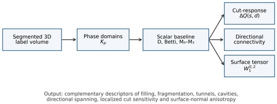
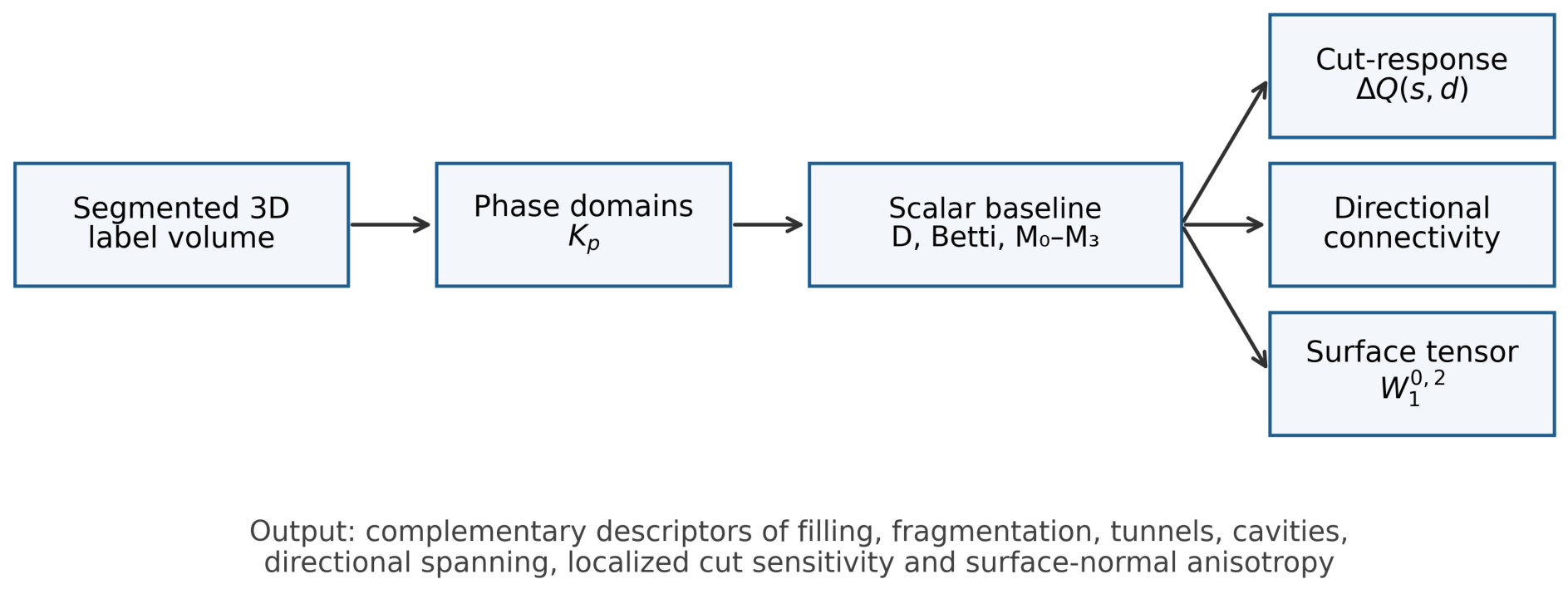
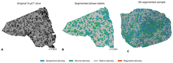
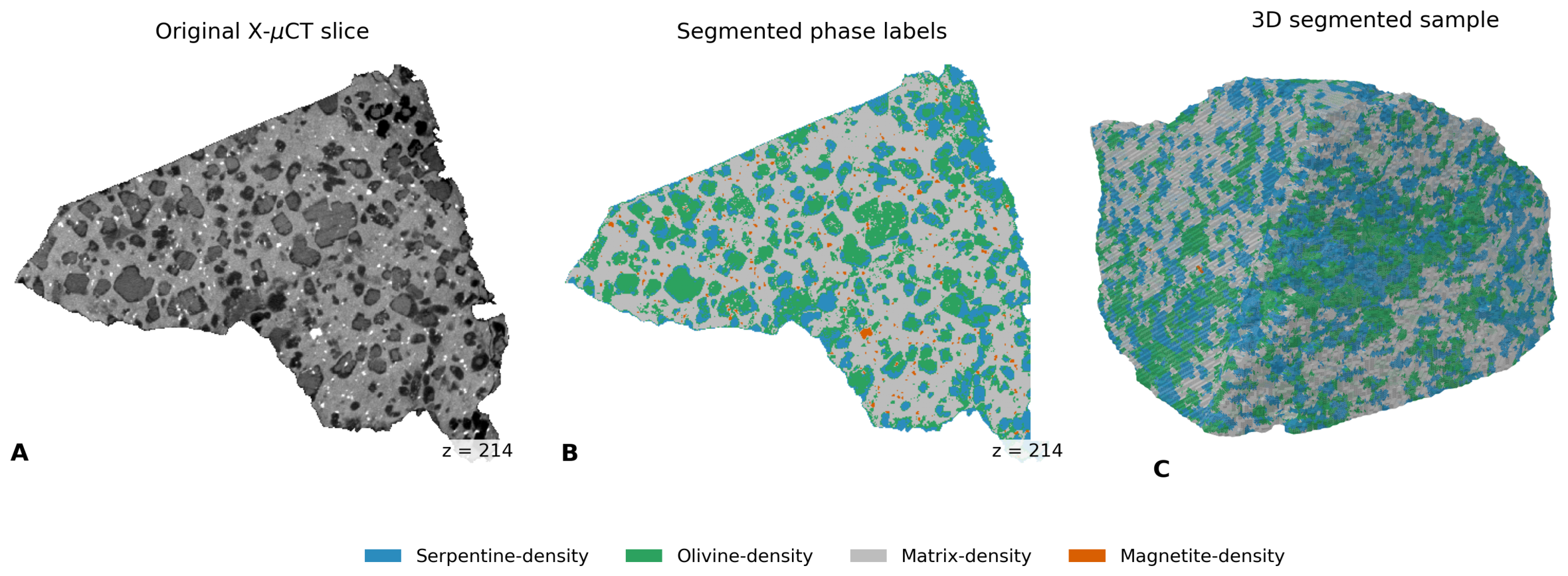
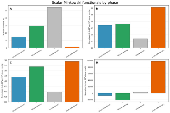
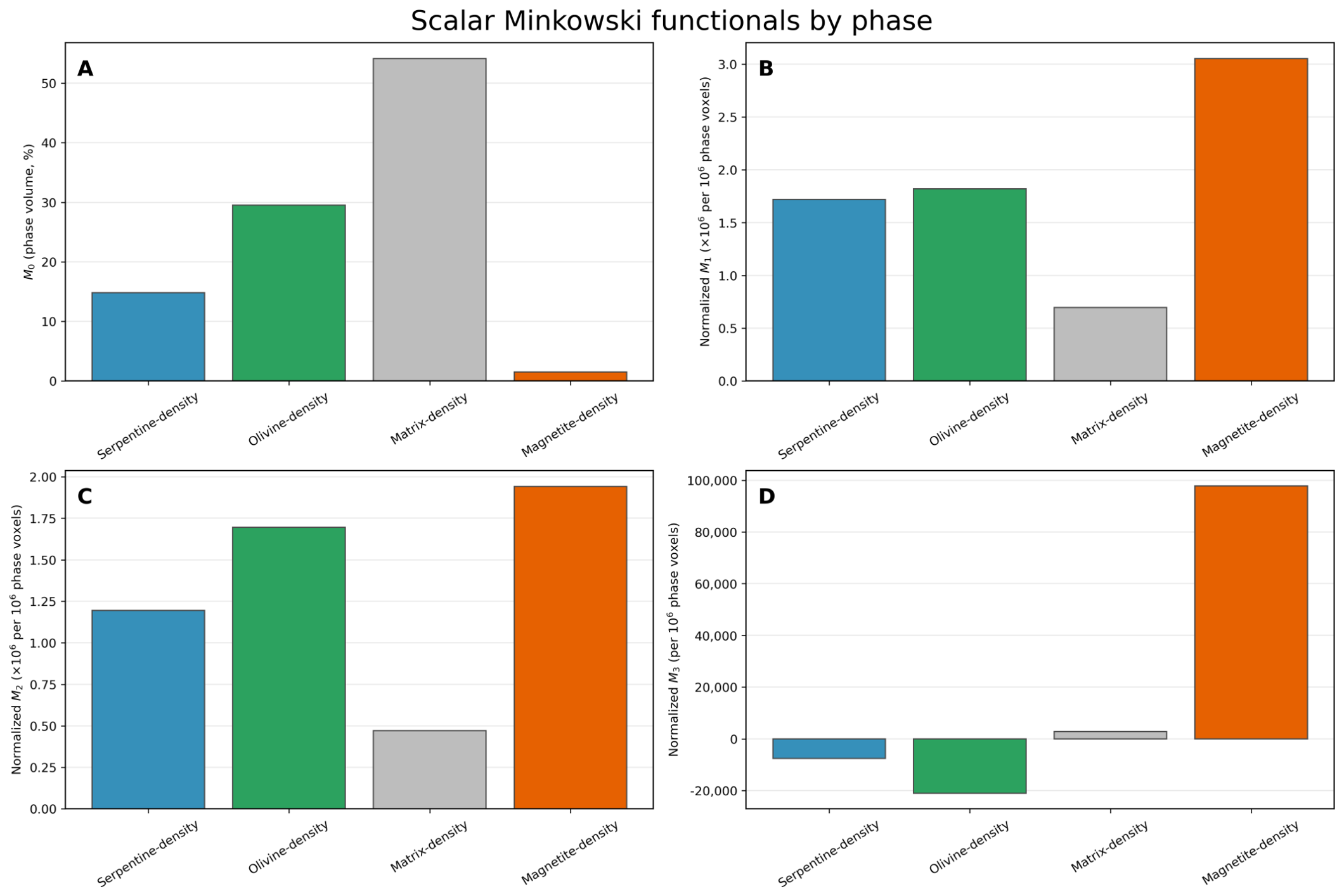
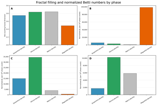
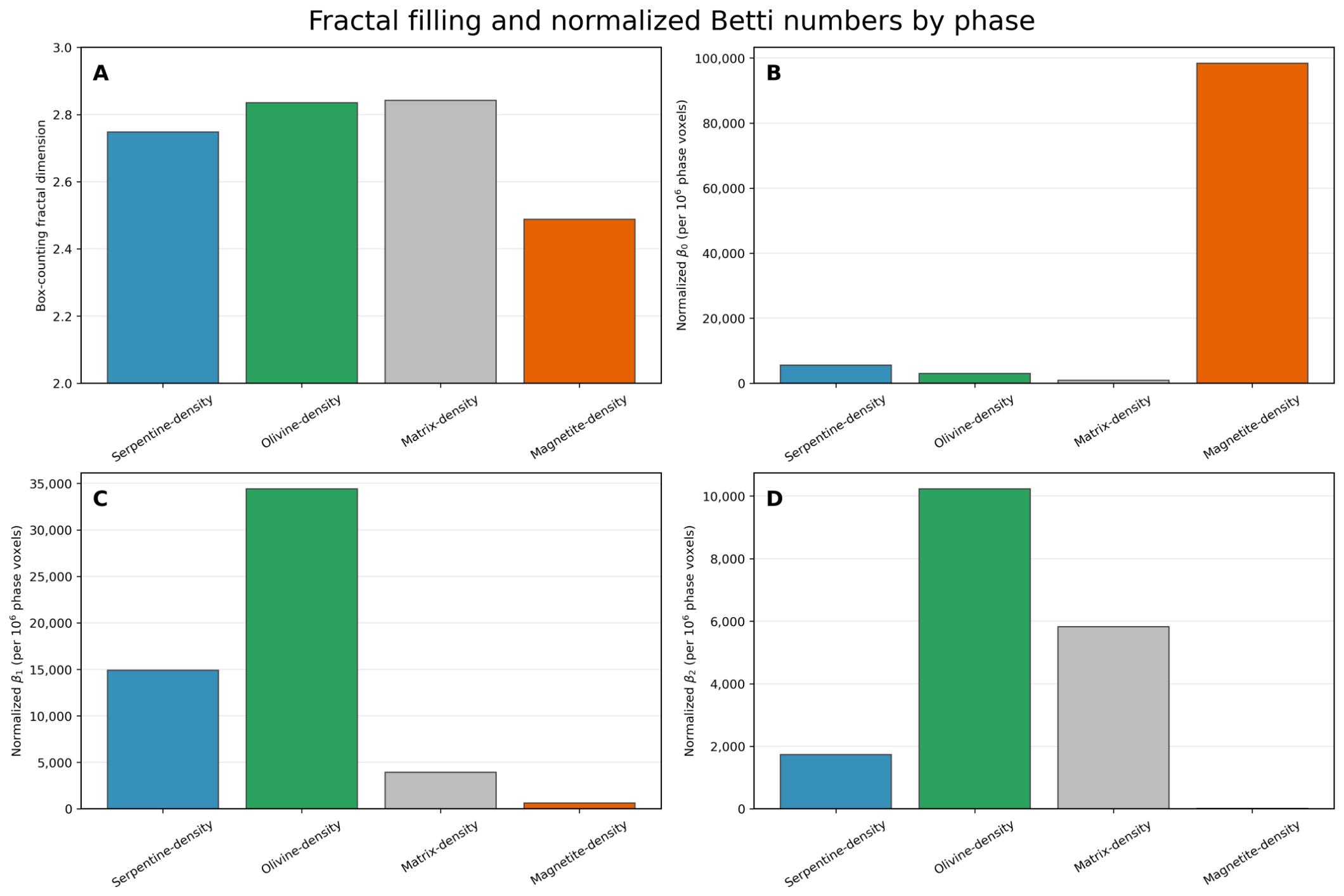
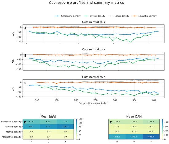
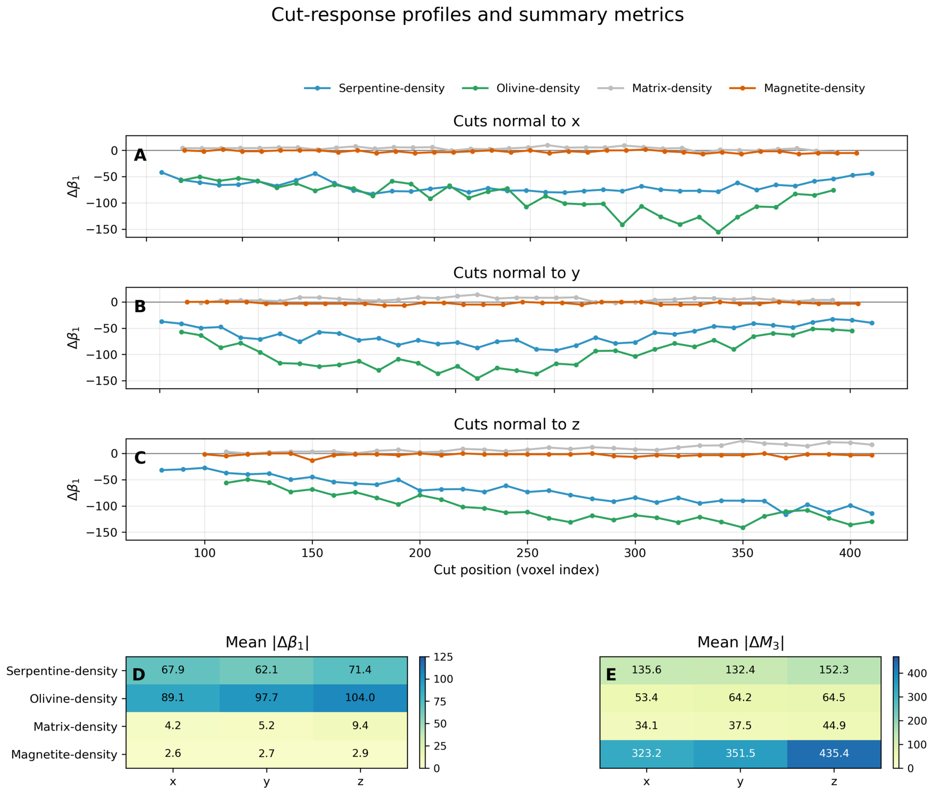
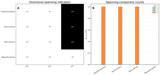
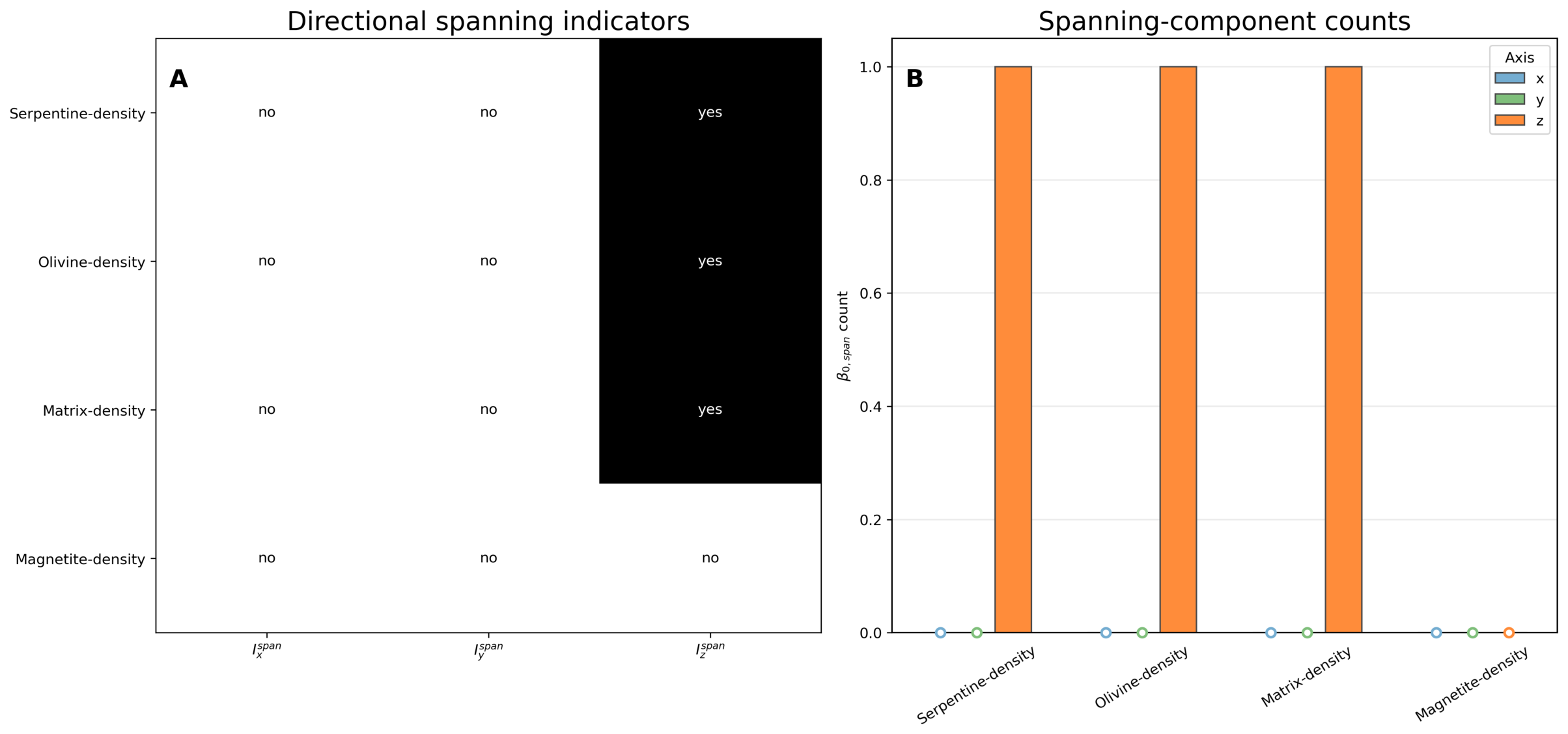
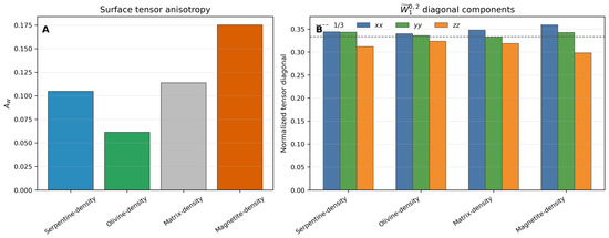
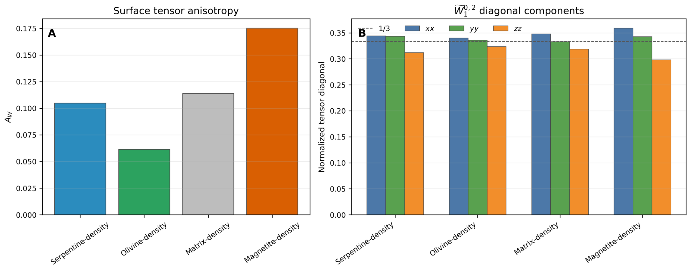
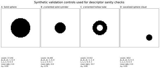
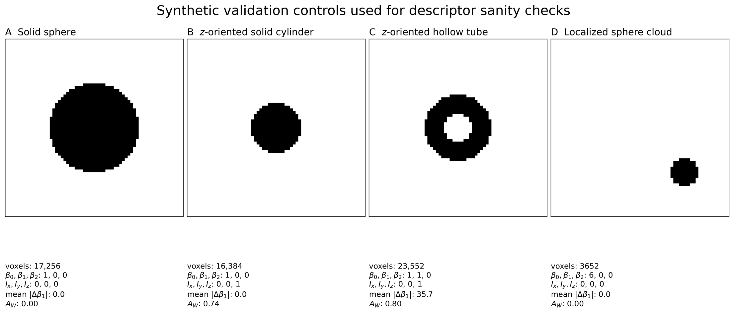
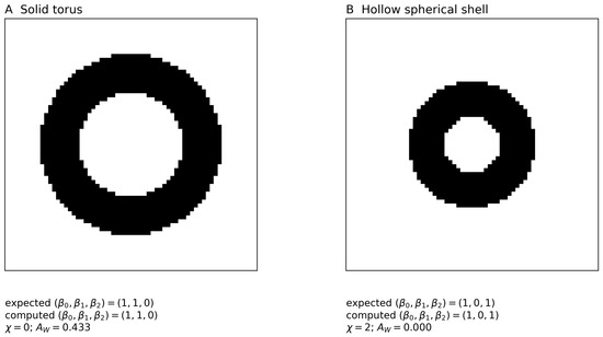
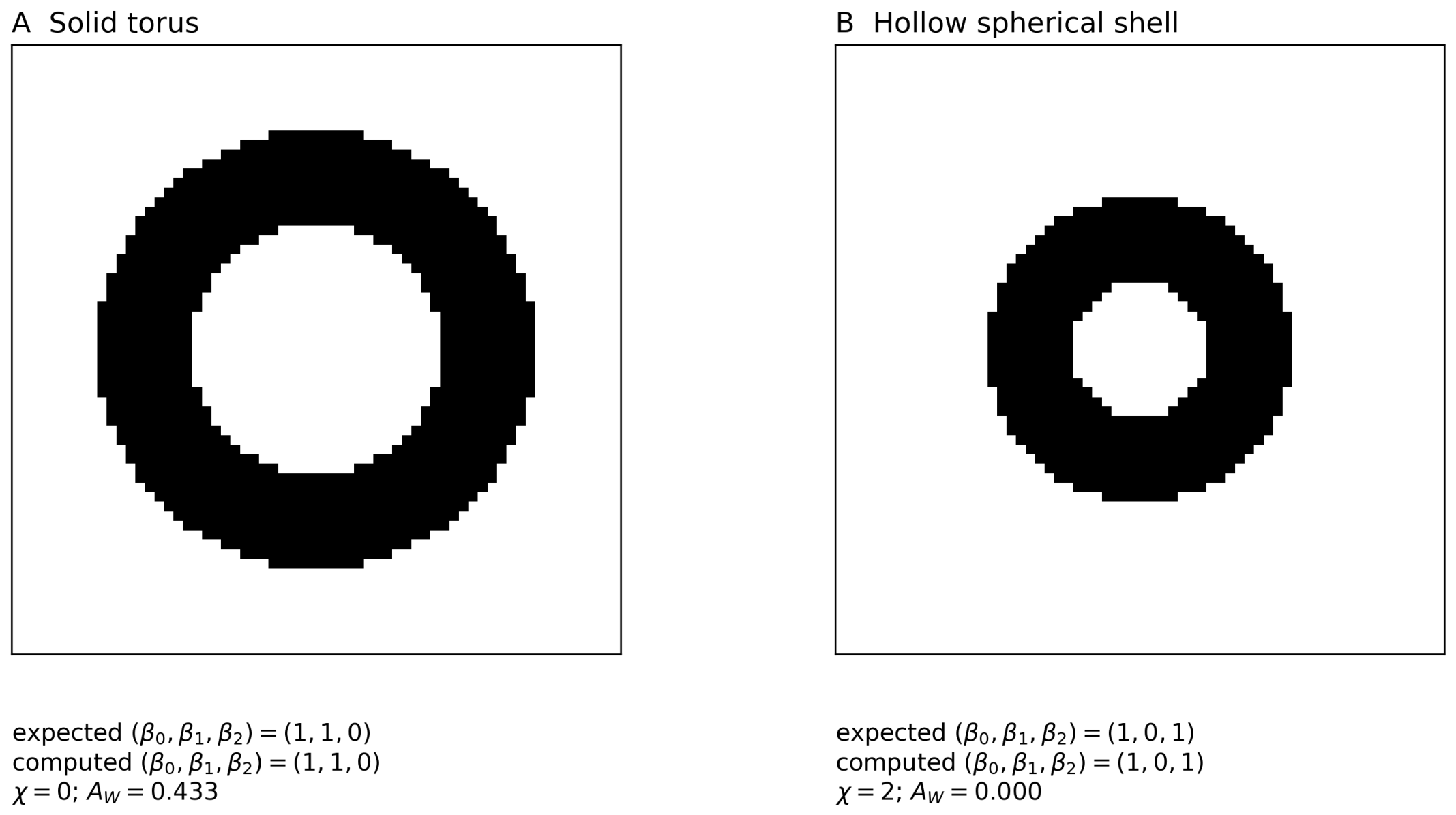

Disclaimer/Publisher’s Note: The statements, opinions and data contained in all publications are solely those of the individual author(s) and contributor(s) and not of MDPI and/or the editor(s). MDPI and/or the editor(s) disclaim responsibility for any injury to people or property resulting from any ideas, methods, instructions or products referred to in the content. |
© 2026 by the authors. Licensee MDPI, Basel, Switzerland. This article is an open access article distributed under the terms and conditions of the Creative Commons Attribution (CC BY) license.