Abstract
The purpose of this paper is to rigorously derive the cubic–quintic Ginzburg–Landau equation as a modulation equation for the stochastic Swift–Hohenberg equation with cubic–quintic nonlinearity on an unbounded domain near a change of stability, where a band of dominant pattern is changing stability. Also, we show the influence of degenerate additive noise on the stabilization of the modulation equation.
1. Introduction
The Swift–Hohenberg equation, which is a nonlinear parabolic equation containing fourth-order space-derivatives, takes the form
Equation (1) was first proposed in 1977 by Swift and Hohenberg [1] as a simple model for the Rayleigh–Benard instability of roll waves. The equation also plays a key role in the studies of pattern formation [2].
Near the change of stability, Kirrmann et al. [3] approximated the solution of the Swift–Hohenberg Equation (1) on an unbounded domain via the Ginzburg–Landau equation
This method of approximation depends on high regularity of the modulation equation, as they needed
In this paper, we consider the stochastic Swift–Hohenberg equation with cubic–quintic nonlinearity defined on an unbounded domain, which reads as follows:
where U is a real-valued scalar function and , , are real coefficients. The coefficients and are chosen to be positive so that is responsible for the subcritical bifurcation of periodic states and is responsible for saturating the growth of the instability. The linear differential operator has eigenvalues for corresponding to eigenfunctions . We have for changing sign a band of uncountably many eigenvalues changing sign around . We perturb the equation for simplicity by a space-independent noise shaking the system uniformly, which is given by the derivative of a standard real-valued Brownian motion .
The deterministic (i.e., ), Swift–Hohenberg Equation (2) has been used to model convective systems with mid-plane and left–right reflection symmetries and yields qualitatively reliable predictions of the properties of localized convection in binary fluids [4,5,6,7] and doubly diffusive convection [8].
Burke et al. [9], Dawes [10] and Hiraoka et al. [11] have studied the bifurcation behavior of the deterministic Equation (2) with the former focusing on the spatially localized states on an extended domain, and the latter focusing on the modulated structures formed on a finite domain. Sakaguchi and Brand [12] have found by computer simulations that the deterministic Equation (2) may have many types of stable localized stationary solutions in suitable parameter regions.
The deterministic Swift–Hohenberg Equation (2) with cubic and quintic nonlinearities is a model equation for describing pattern forming systems near instabilities with non-trivial spatial wavelength [13]. Since many dynamical systems are subject to the influence of noise, it is desirable to incorporate this influence into the mathematical model. The analysis of the effect of the noise on the properties of the solution and its approximation by a corresponding modulation equation become very relevant in this context.
Our aim in this paper is to rigorously derive the modulation Equation (3) which is called the cubic–quintic Ginzburg–Landau equation
and to show that the approximation of the mild solutions U of Equation (2) by a modulated wave-train of the form
where is the solution of the Ginzburg–Landau Equation (3) which is defined on the slow time and “slow” space . The perturbation is a fast Ornstein–Uhlenbeck process, defined as
where is a rescaled version of the Brownian motion.
Also, our purpose is to treat the modulation equation with space–time white noise with least possible regularity. Although in our situation the solution of the modulation Equation (3) is spatially smooth, but is only Hölder in time.
In our previous paper [14] (written in collaboration with D. Blömker and K. Klepel), we studied the simpler case of a stochastic Swift–Hohenberg Equation (2), when and on unbounded domain and we established rigorously the following modulation equation
For more results on the stochastic Swift–Hohenberg equation, see for instance [15,16,17]. Moreover, the generalized Swift–Hohenberg equation with simpler quadratic nonlinearity of the type is treated in [18].
The paper is divided into the following sections. In the next section we define the space and mild solution of Equation (2). In Section 3 we give a formal derivation of the modulation equation. In Section 4 we give general bounds on the Ornstein–Uhlenbeck process . In Section 5 we state and prove the main result of this paper. In Section 6, we show the effect of the degenerate additive noise on the stabilization of the modulation equation of the Swift–Hohenberg Equation (2). Finally, we give conclusions of this paper.
2. Space and Mild Solution
In this paper we will work in the following well known Sobolev space , see [19].
Definition 1.
For we define the space by
with norm
where is the Fourier transform of u, defined by
Note that in the space functions still decay to 0 at ∞. Thus if we are still in a setting, where the solutions of Equation (2) and the amplitude A decay to 0 for .
Definition 2.
(Mild solution) Let be a time. The continuous stochastic process is called a mild solution of Equation (2) if
where is initial function.
The existence of the mild solution of Equation (6) is standard by using a fixed point arguments for example in the space for sufficiently smooth noise.
In next definition we state what we mean exactly when we write “order of” or its abbreviation .
Definition 3.
For a family of real-valued stochastic processes we say , if for every there exists a constant such that
where is the norm in . The similar notation is also used for time-independent random variables.
3. Derivation of Cubic–Quintic Ginzburg–Landau Equation
Before we discuss a formal derivation of the amplitude or modulation equation corresponding to Equation (2). Let us state the following lemma without proof (see the proof of Lemma 5.1 in [20]) on averaging over the fast OU-process where for (see the proof of Lemma 4.2 in [20]). This lemma displays that the integrals over the OU-process contains even powers like or and have a contribution, which is a constant of order one. While the integrals contain odd powers like or are small.
Lemma 1.
Let be a complex valued stochastic process and for . If , with , then for and
Now, we assume that a solution of the modulation Equation (3) is sufficiently smooth. First, let us introduce a small parameter and define the parameters and in Equation (2) as
This means that one actually considers the equation
If we rescale to the slow time-scale and slow spatial scale via
then Equation (9) takes the form
where and . Now define w as
Let us make the following ansatz:
where denotes the complex conjugate. The additional higher order terms do not improve the approximation result, but they are necessary to eliminate large error terms.
Plugging Equation (13) into Equation (12), assuming that all terms are sufficiently smooth, and using the relation
we obtain
In order to remove all unwanted terms, define
Hence
Collecting all terms in front of , yields
To obtain the modulation Equation (3), we ignore all small terms in .
4. General Bounds on OU Process
In this section we give a general bound on Ornstein–Uhlenbeck process
Lemma 2.
Proof.
Let for
Hence
Using Equation (3), we obtain
Define
Taking for both sides and using the following two inequalities (Theorem 5.4 in [19]) and (Corollary 4.6 in [14]), yields
Hence
Lemma 3.
If A is the solution of the mild formulation of Equation (3) with for , and for , then
5. Main Results
In this section, we state and prove the main result of this paper. First, let us state without proof two lemma’s from [14]. The purpose of the first one is to change the semigroup by the semigroup when they are applied to a modulated wave , while the purpose of the second one is to bound the semigroup when applied to
Lemma 4.
There is a constant such that, for and for we have
where is defined as
Let and . There are two constants and depending on such that, for and ,
Next let us define and bound the residual.
Definition 4.
Lemma 5.
Proof.
From Equation (25), we obtain
In this step we used the bound on (where ) and the bound terms like .
Now, using Lemma 4 for changing the semigroup and Lemma 5 to bound terms like , yields
where is defined in Equation (23). From the modulation Equation (3) we have
Using Lemmas 2 and 3, yields Equation (27) for , which is always true for if we choose sufficiently small. □
Definition 5.
Define the set such that for sufficiently small and for all , all these estimates
and
hold on.
Proposition 1.
For all , there exist a constant such that on
Proof.
Using Chebychev’s inequality
From Lemmas 2, 3 and 5, we obtain
For sufficiently large q, yields
□
The main result of this paper is the following approximation result for solutions of the stochastic Swift–Hohenberg Equation (9) through the solutions of the Ginzburg–Landau Equation (3).
Theorem 1.
(Approximation) Let be a solution of Equation (9), the formal approximation defined in Equation (26) such that and for and for . Suppose that for the initial function
for some fixed constant and for some small . Then for each such that for all there exist depending on such that
where the fast OU process defined in Equation (5) and defined in Equation (23).
Proof.
We follow the same steps of the proof of Theorem 3.4 in [14]. □
6. The Effect of Degenerate Additive Noise
In this section we show the effect of degenerate additive noise on the stabilization of the solution of the Ginzburg–Landau Equation (3). Let us first fix , and . Therefore, in the modulation Equation (3), we note in this case that:
- The coefficient of the cubic term is positive for and is a non-positive otherwise,
- The coefficient of the linear term is positive for if or if and is a non-positive otherwise.
Now, some numerical simulations are presented for the fixed parameters and varying noise intensity . We carried out a straightforward semi-implicit time discretization of the Galerkin spectral method using fast Fourier transforms. For time discretization, we used a constant small time step, for example, .
In the Figure 1, we see that the modulation equation solution fluctuates and has a pattern if the noise intensity .
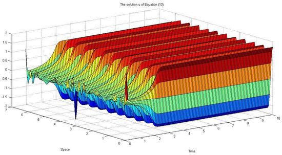
Figure 1.
, and .
In Figure 2, Figure 3, Figure 4 and Figure 5, if the noise intensity of increases, the pattern begins to destroy due to the noise effect.
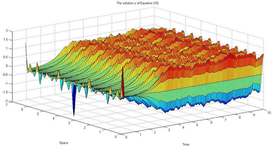
Figure 2.
, and .
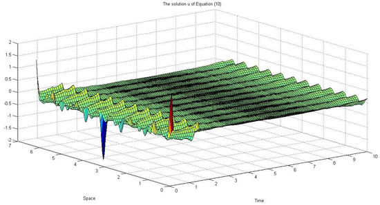
Figure 3.
, and .
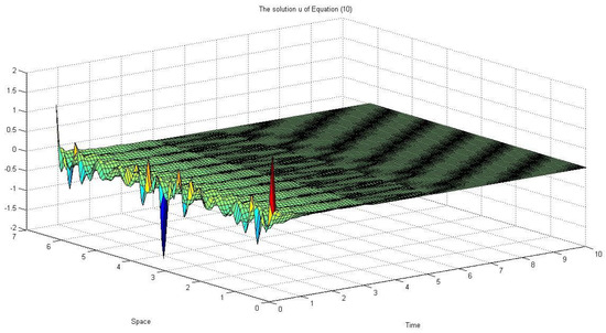
Figure 4.
, and .
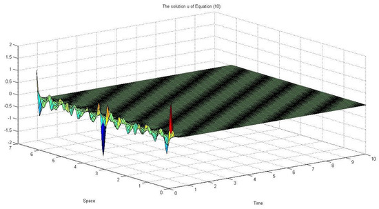
Figure 5.
, and .
If we choose if or if , then the coefficient of the linear term is negative. Therefore, we deduce that small global noise has the potential to stabilize the modulation equation, and thus to destroy the dominant pattern.
7. Conclusions
In this paper, we considered the stochastic Swift–Hohenberg Equation (1) with cubic–quintic nonlinearity defined on an unbounded domain and derived rigorously the Ginzburg–Landau equation as a modulation Equation (3). Near change of stability, we approximated the solution of the Swift–Hohenberg Equation (1) by the solution of the Ginzburg–Landau Equation (3). Finally, we showed the effect of the degenerate additive noise on the stabilization of the solution of the modulation Equation (3).
Funding
This research received no external funding.
Acknowledgments
We would like to express our sincere thanks to the referees for their constructive comments on improving this paper.
Conflicts of Interest
The authors declare no conflict of interest.
References
- Swift, J.B.; Hohenberg, P.C. Hydrodynamic fluctuations at the convective instability. Phys. Rev. A 1977, 15, 319–328. [Google Scholar] [CrossRef]
- Cross, M.C.; Hohenberg, P.C. Pattern formation outside of equilibrium. Rev. Mod. Phys. 1993, 65, 536–1112. [Google Scholar] [CrossRef]
- Kirrmann, P.; Schneider, G.; Mielke, A. The validity of modulation equations for extended systems with cubic nonlinearities. Proc. R. Soc. Edinb. Sect. A 1992, 122, 85–91. [Google Scholar] [CrossRef]
- Batiste, O.; Knobloch, E.; Alonso, A.; Mercader, I. Spatially localized binary fluid convection. J. Fluid Mech. 2006, 560, 149–158. [Google Scholar] [CrossRef]
- Lo Jacono, D.; Bergeon, A.; Knobloch, E. Spatially localized binary fluid convection in a porous medium. Phys. Fluids 2010, 22, 073601. [Google Scholar] [CrossRef]
- Mercader, I.; Batiste, O.; Alonso, A.; Knobloch, E. Convectons, anticonvectons and multiconvectons in binary fluid convection. J. Fluid Mech. 2011, 667, 586–606. [Google Scholar] [CrossRef]
- Mercader, I.; Batiste, O.; Alonso, A.; Knobloch, E. Traveling convections in binary fluid convection. J. Fluid Mech. 2013, 722, 240–266. [Google Scholar] [CrossRef]
- Beaume, C.; Bergeon, A.; Knobloch, E. Homoclinic snaking of localized states in doubly diffusive convection. Phys. Fluids 2011, 23, 094102. [Google Scholar] [CrossRef]
- Burke, J.; Knobloch, E. Snakes and ladders: Localized states in the Swift–Hohenberg equation. Phys. Lett. A 2007, 360, 681–688. [Google Scholar] [CrossRef]
- Dawes, J.H. Modulated and localised states in a finite domain. SIAM J. Appl. Dyn. Syst. 2009, 8, 909–930. [Google Scholar] [CrossRef][Green Version]
- Hiraoka, Y.; Ogawa, T. Rigorous numerics for localized patterns to the quintic Swift–Hohenberg equation. Jpn. J. Indust. Appl. Math. 2005, 22, 57–75. [Google Scholar] [CrossRef]
- Sakaguchi, H.; Brand, H.R. Stable localized solutions of arbitrary length for the quintic Swift–Hohenberg equation. Physica D 1996, 97, 274–285. [Google Scholar] [CrossRef]
- Avitabile, D.; Lloyd, D.J.; Burke, J.; Knobloch, E.; Sandstede, B. To snake or not to snake in the planar Swift–Hohenberg equation. SIAM J. Appl. Dyn. Syst. 2010, 9, 704–733. [Google Scholar] [CrossRef]
- Mohammed, W.W.; Blömker, D.; Klepel, K. Modulation equation for stochastic Swift–Hohenberg equation. SIAM J. Math. Anal. 2013, 45, 14–30. [Google Scholar] [CrossRef]
- Blömker, D.; Hairer, M.; Pavliotis, G.A. Modulation equations: Stochastic bifurcation in large domains. Commun. Math. Phys. 2005, 258, 479–512. [Google Scholar] [CrossRef]
- Hutt, A. Additive noise may change the stability of nonlinear systems. Europhys. Lett. 2008, 84, 1–4. [Google Scholar] [CrossRef]
- Hutt, A.; Longtin, A.; Schimansky-Geier, L. Additive global noise delays Turing bifurcations. Phys. Rev. Lett. 2007, 98, 230601. [Google Scholar] [CrossRef] [PubMed]
- Klepel, K.; Blömker, D.; Mohammed, W.W. Amplitude equation for the generalized Swift Hohenberg equation with noise. Zeitschrift für Angewandte Mathematik und Physik ZAMP 2014, 65, 1107–1126. [Google Scholar] [CrossRef][Green Version]
- Adams, R.A. Sobolev Spaces; Academic Press: New York, NY, USA, 1975. [Google Scholar]
- Blömker, D.; Mohammed, W.W. Amplitude equations for SPDEs with cubic nonlinearities. Int. J. Probab. Stoch. Process. 2013, 85, 181–215. [Google Scholar] [CrossRef][Green Version]


© 2019 by the author. Licensee MDPI, Basel, Switzerland. This article is an open access article distributed under the terms and conditions of the Creative Commons Attribution (CC BY) license (http://creativecommons.org/licenses/by/4.0/).