Article

Similarity Measures for Fractional Orthotriple Fuzzy Sets Using Cosine and Cotangent Functions and Their Application in Accident Emergency Response

by
Muhammad Naeem
1,
Muhammad Qiyas
2,
Mohammed M. Al-Shomrani
3 and
Saleem Abdullah
2,*
1
Deanship of Combined First Year Umm Al-Qura University Makkah, Mecca, P.O. Box 715, Saudi Arabia
2
Department of Mathematics, Abdul Wali Khan University, Mardan 23200, Pakistan
3
Department of Mathematics, Faculty of Science, King Abdulaziz University, P.O. Box 802000, Jeddah 21589, Saudi Arabia
*
Author to whom correspondence should be addressed.
Mathematics 2020, 8(10), 1653; https://doi.org/10.3390/math8101653
Submission received: 6 August 2020 / Revised: 28 August 2020 / Accepted: 3 September 2020 / Published: 24 September 2020

Abstract

:
The fractional orthotriple fuzzy set (FOFS) is more generalized than the spherical fuzzy set (SFS) and picture fuzzy set (PFS) to cope with awkward and complex information in fuzzy set (FS) theory. The FOFS is a more powerful technique with respect to the existing drawbacks because of its conditions, i.e., the sum of the f powers of positive, neutral, and negative grades is bounded to [ 0 , 1 ] . With the advantages of the FOFS, in this paper, we study the basic definitions and some existing similarity measures (SMs) of intuitionistic fuzzy sets (IFSs), PFSs, Pythagorean fuzzy sets (PyFSs) and SFSs. The existing approaches have certain limitations and cannot be applied to problems that are in the form of FOFSs. The goal of this paper is to propose the idea of some new SMs including cosine SMs for FOFSs, SMs for FOFSs based on the cosine function, and SMs for FOFSs based on the cotangent function. Further, some weighted SMs (WSMs) are also proposed for which the weight of the attributes is considered. Then, we apply these SMs and WSMs to the pattern recognition problem. Finally, the comparative study of the new SMs for FOFSs is established with existing SMs, and also, some advantages of the proposed work are discussed.

1. Introduction

In practical decision making problems (DMPs), there are many uncertainties, and much imprecise and vague information, the representations and management of which are always the central issues. Health professionals and health care administrators are working to reduce the clinical and maintenance costs in the prevention and management of coronavirus disease. The expenditures of and need for health care are both growing fast. Health care practitioners, administrators, and other sectors collectively perform a range of health care management techniques with the goal to facilitate effective disease prevention approaches using scarce resources. Such principles are used to build a decision-making model with a number of parameters and alterna- tives. The purpose of multi-criteria decision-making (MCDM) frameworks to make appropriate decisions at different levels of health care, such as operational, methodological, and functional. There may be an ideal solution to a difficult decision-making (DM) problem, but it is a difficult task to find such a solution.
Zadeh [1] in 1965, defined the theory of fuzzy sets (FSs). FSs are a great achievement and have some applications in various fields. An FS is based on a characteristic function that has its membership grade denoted by σ for each number of X (universal set) in the closed interval from zero to one. Atanassov’s [2] generalized the idea of FS to the idea of intuitionistic fuzzy sets (IFSs). An IFS has two functions, positive and negative membership grades denoted by σ and υ for each element of the universal X in the closed-interval from zero to one. Further, the sum of σ and υ must belong to [ 0 , 1 ] , i.e., s u m σ , υ [ 0 , 1 ] . If we take σ = 0.7 and υ = 0.4 , respectively, then 0.7 + 0.4 = 1.15 > 1 . In this situation, the IFSs cannot explain such details. Therefore, due to this limitation, Yager [3,4] developed the notion of Pythagorean fuzzy sets (PyFSs) by increasing the domain of IFSs. A PyFS also has two functions, positive and negative membership grades denoted by σ and υ for each element of the universal X in the closed interval [ 0 , 1 ] . The sum of squares of σ and υ belongs in the closed interval [ 0 , 1 ] , i.e., s u m σ 2 , υ 2 [ 0 , 1 ] . Therefore, the PyFS is the generalization of the IFS because the domain of the PyFS is larger than the IFS. For some other recent studies on IFSs and PyFSs, one may refer to Asiain et al. [5], Mahmood et al. [6], Li [7], Peng and Yang [8], Garg [9], Wei and Lu [10] and Lu et al. [11,12].
In the case of IFSs we know that human opinion only has option types of yes or no. Therefore, due to this limitation, Cuong [13] introduced the idea of picture fuzzy sets (PFSs) and described their basic operations and properties. In this case, human opinion have four option types, i.e., yes, no, abstain, and refusal. A PFS has three types of functions, membership, abstain, and non-membership grades denoted by σ , η and υ for each element of the universal set X in the closed-interval [ 0 , 1 ] . In the PFS, the sum of σ , η and υ must belong on the closed-interval [ 0 , 1 ] , i.e., s u m σ , η , υ [ 0 , 1 ] . Therefore, it is proven that the PFS is the direct generalization of the FS and IFS. Akram et al. [14] proposed a decision-making model under complex picture fuzzy Hamacher aggregation operators. Ahmad et al. [15] introduced some operations on interval-valued PFSs (IVPFSs), IVPF soft sets, and their applications. Garg [16] developed some picture fuzzy aggregation operators and an approach for multi-criteria decision-making. Lin et al. [17] proposed a novel picture fuzzy mult-attribute decision making (MADM) approach using the extended Multiple Objective Optimization on the basis of Ratio Analysis plus Full Multiplicative Form (MULTIMOORA) technique to solve the site selection for a car sharing station. Liu et al. [18] defined similarity measures (SMs) for IVPFSs and discussed their applications in DMPs. For some other recent studies in these areas, one may refer to [19,20].
PFS extended the Zadeh concept of FS and Atanassov’s idea of IFS, but still there is a limitation of this structure such as if we take σ = 0.5 , η = 0.3 and υ = 0.4 respectively, then it is enough. Because, in PFS, we know that the values cannot be allowed to its characteristic functions independently. So due this limitation Mahmood et al. [21] defined the idea of SFS by increasing the domain of PFS. A SFS has also three functions, positive, abstinence and negative grades denoted by σ , η and υ for each element of the universal X on the closed-interval [ 0 , 1 ] . The sum of squares of σ , η and υ belong on the closed-interval [ 0 , 1 ] , i.e., s u m σ 2 , η 2 , υ 2 [ 0 , 1 ] . Therefore, SFS is the generalization of PFS because the domain of SFS is larger than PFS. However, sometimes, if we take σ = 0.6 , η = 0.7 and υ = 0.8 respectively, then it is enough because the sum of squares of them is larger than 1. For some related work on SFS one we may refer to [22,23,24,25,26,27,28].

1.1. Literature Review

SM is an interesting topic in fuzzy mathematics that tells us the degree of similarity of two objects. SMs can be utilized in pattern recognition’s [29,30,31], medical diagnosis [32,33], group decision making [34] and clustering analysis [35] etc. Ye [36] proposed cosine SMs of IFSs. Rajarajeswari and Uma [37] introduced the cotangent SM of IFSs and Ye [38] developed SMs of IFS using the cosine function. Further, Wei [39] introduced the concept of SMs for PFSs. Wei [40] proposed cosine SMs for PFSs and Ahmad et al. [41] developed the concept SMs for picture hesitant fuzzy set (PHFS) and their applications. Moreover, Wei et al. [42] defined SMs of PyFS using cosine function and Ullah et al. [43] developed SMs for FOFS with applications. Recently, Wei et al. [42] proposed the SMs of SFS using the cosine function. Shougi et al. [44] defined a three-way DM using covering based FOF Rough Set Model.
The idea of similarity is a fundamental notion in human attention. SM plays an significant role in taxonomy, identification etc. There are many condition of the similarity notion that have eluded formalization. Under [picture fuzzy set] of a true, general purpose similarity description is a challenging problem. There is no true, general purpose definition of similarity. There are some special purpose definitions in cluster analysis, search, classification, recognition and diagnosis that have been used successfully. The tests of similarity are divided into three groups: (1) metric based measures, (2) set-theoretic based measures and (3) implication based measures. In dealing with distance-based SMs, examples have been constructed of perceptual similarity where distance axiom is clearly violated by dissimilarity measures, in particular triangular inequalities, and consequently the resulting SM disobeys transitivity. This study suggests that the perceptual distance satisfies the metric axioms of which many researchers have experimentally questioned the empiric validity, in particular the triangular inequality. Similarly, for set theoretical similarity measurements, it is noticed that crisp transitivity is a more stronger requirement for similarity measurement. Set theoretical similarity measurements are subdivided further into three classes (a) measures based on a crisp logic (b) measures based on a fuzzy logic (c) measures based on a hesitant fuzzy set.

1.2. Motivation and Novelties

The function of fractional orthotriple fuzzy sets (FOFS) in the DMP is very important among the other extensions of FSs. In FOFSs, the viewpoint is not only limited to yes or no, but also to some kind of denial or abstinence. The FOFS is a very useful tool for explaining the object without ambiguity, while in the other tool the knowledge is complex and uncertain. For example, we assume that a country wants to build or launch a medical treatment or health care center project. The government party will offer high support for its proposal, the government allocated membership grade of 0.8 per cent, while the opposition party will approve it, if the same proposal is not pleasant, they will strongly oppose it. The minority party would allocate 0.75 . to non-membership. The other small party will remain neutral and will be given a membership grade of 0.2 , in case of a PFS, 0.8 + 0.2 + 0.75 = 1.75 > 1 , in this case the PFS could not clarify this detail. Now, assume that an SFS, ( 0.8 ) 2 + ( 0.75 ) 2 + ( 0.2 ) 2 = 1.243 > 1 , in this scenario, too, the SFS failed to justify such details. In case of FOFS, ( 0.8 ) f + ( 0.75 ) f + ( 0.2 ) f 1 , where f Q + . In order to resolve this issue of confusion, we need a detailed method to explain this form of problem during the decision-making process. Keeping the advantages of the SM, in this article, we studied basic definitions and some existing SMs of PyFSs, PFSs and SFSs. However, the existing approaches have some limitations and could not be applied on those problems in which there data occur in the form of FOFNs. This article aims to developed the notion of some new SMs including cosine SM (WSMs) for FOFSs using the cosine function and SMs (WSMs) for FOFSs using the cotangent function. Then, we apply these SMs and WSMs to pattern recognition problem. Finally, the comparative analysis of the new SMs (WSMs) for FOFSs is developed with the existing SMs (WSMs).
Thus, we observed that the existing SMs of PyFSs and SFSs have some limitation and cannot be applied to those problems whose environment is FOFSs. To deal with this issue, we proposed SMs (WSMs) for FOFSs using the cosine function and cotangent function which are the direct generalization of References [42,43,45]. Therefore, the references [42,43,45] will become the special cases of the defined SMs (WSMs).
The remainder of the paper is arranged as: In Section 1, the history of existing concepts is discussed in detail. In Section 2, we discussed some basic definitions of IFSs, PyFSs, PFSs, SFSs and FOFSs. In Section 3, we propose SMs and weighted SMs based on cosine function for FOFSs. In Section 4, the SMs developed in Section 3 are applied to pattern recognition. In Section 5, the comparative study of the proposed work is discussed. Finally, the article is summarized with some future directions.

2. Preliminaries

In this portion, we studied basic definitions and notion related to IFSs, PyFSs, PFSs, SFSs, FOFSs and some SMs. In our study by X we mean the universal set and σ , η , υ and γ denote the positive, abstinence, negative and refusal grades on the closed-interval [ 0 , 1 ] . Moreover, the notation “∨” is denote the maximum operation and the set of FOFNs on X are represented by F O F S ( X ) .
Definition 1.
An IFS ℑ on X is of the shape = , σ ( ) , υ ( ) | X provided that 0 s u m σ ( ) , υ ( ) 1 . Further, γ ( ) = 1 s u m σ ( ) , υ ( ) is called the refusal grade of X in . For convenience σ , υ is called an intuitionistic fuzzy number (IFN) [2].
Definition 2.
A PyFS on X is of the shape = , σ ( ) , υ ( ) | X provided that 0 s u m σ 2 ( ) , υ 2 ( ) 1 . Further, γ ( ) = 1 s u m σ 2 ( ) , υ 2 ( ) is known the refusal grade of X in . For convenience σ , υ is called a Pythagorean fuzzy number (PyFN) [3,4].
Definition 3.
A PFS ℑ on X is of the shape = , σ ( ) , η ( ) , υ ( ) | X provided that 0 s u m σ ( ) , η ( ) , υ ( ) 1 . Further, γ ( ) = 1 s u m σ ( ) , η ( ) , υ ( ) is called the refusal grade of X in . For convenience σ , η , υ is called a picture fuzzy number (PFN) [13].
Definition 4.
A SFS on X is of the shape = , σ ( ) , η ( ) , υ ( ) | X provided that 0 s u m σ 2 ( ) , η 2 ( ) , υ 2 ( ) 1 . Further, γ ( ) = 1 s u m σ 2 ( ) , η 2 ( ) , υ 2 ( ) is called the refusal grade of X in . For convenience σ , η , υ is called a spherical fuzzy number (SFN) [21].
Definition 5.
A FOFS ℑ on X is of the shape = , μ , η , ν | X provided that s u m μ f + η f + ν f 1 . Further π = 1 s u m σ f ( ) , η f ( ) , υ f ( ) f is called the refusal grade of X in . For convenience, μ , η , ν is said to be a fractional orthotriple fuzzy number (FOFNs) [44].
Remark 1.
We know that if
∘ we put f = 2 in definition (5), then FOFS reduces to SFS
∘ we put f = 1 in definition (5), then FOFS reduces to PFS
∘ we put f = 2 and η = 0 in definition (5), then FOFS reduces to PyFS
∘ we put f = 1 and η = 0 in definition (5), then FOFS reduces to IFS
∘ we put f = 1 and η = υ = 0 in definition (5), then FOFS reduces to FS
This remark identifies that SFS, PyFS, PFS, IFS, and FS are the special cases of FOFS [44].
Definition 6.
For two IFNs = σ , υ and = σ , υ on X , a cosine SM is defined as [36]
I F C 1 , = 1 m i = 1 m σ ( i ) σ ( i ) + υ ( i ) υ ( i ) σ 2 ( i ) + υ 2 ( i ) σ 2 ( i ) + υ 2 ( i )
Definition 7.
For two PFNs = σ , η , υ and = σ , η , υ on X , a cosine SM is described as [39]
P F C 1 , = 1 m i = 1 m σ ( i ) σ ( i ) + η ( i ) η ( i ) + υ ( i ) υ ( i ) σ 2 ( i ) + η 2 ( i ) + υ 2 ( i ) σ 2 ( i ) + η 2 ( i ) + υ 2 ( i )
Definition 8.
For any two PFNs = σ , η , υ and = σ , η , υ on X , based on the cosine function, then SM is defined as [40]
P F C S 1 ( , ) = 1 m i = 1 m cos π 2 σ ( i ) σ ( i ) η ( i ) η ( i ) υ ( i ) υ ( i )
P F C S 2 ( , ) = 1 m i = 1 m cos π 4 σ ( i ) σ ( i ) + η ( i ) η ( i ) + υ ( i ) υ ( i )
Definition 9.
For any two PFNs = σ , η , υ and = σ , η , υ on X , based on the cotangent function, then SM is defined as [40]
P F C T 1 ( , ) = 1 m i = 1 m cot π 4 + π 4 σ ( i ) σ ( i ) η ( i ) η ( i ) υ ( i ) υ ( i )
P F C T 2 ( , ) = 1 m i = 1 m cot π 4 + π 4 σ ( i ) σ ( i ) η ( i ) η ( i ) υ ( i ) υ ( i ) γ ( i ) γ ( i )
Definition 10.
For any two PyFNs = σ , υ and = σ , υ on X , a cosine SM is defined as [42]
P y F C 1 , = 1 m i = 1 m σ 2 ( i ) σ 2 ( i ) + υ 2 ( i ) υ 2 ( i ) σ 4 ( i ) + υ 4 ( i ) σ 4 ( i ) + υ 4 ( i )
Definition 11.
For any two PyFNs = σ , υ and = σ , υ on X based on the cosine function, then SM is defined as [42]
P y F C 1 , = 1 m i = 1 m cos π 2 ( | σ 2 ( i ) σ 2 ( i ) | | υ 2 ( i ) υ 2 ( i ) | )
Definition 12.
For any two PyFNs = σ , υ and = σ , υ on X based on the cotangent function, then SM is defined as [42]
P y F C 1 , = 1 m i = 1 m cot π 4 + π 4 ( | σ 2 ( i ) σ 2 ( i ) | | υ 2 ( i ) υ 2 ( i ) | )
Definition 13.
For any two SFNs = σ , η , υ and = σ , η , υ on X , a cosine SM is defined as [42]
S F C 1 , = 1 m i = 1 m σ 2 ( i ) σ 2 ( i ) + η 2 ( i ) η 2 ( i ) + υ 2 ( i ) υ 2 ( i ) σ 4 ( i ) + η 4 ( i ) + υ 4 ( i ) σ 4 ( i ) + η 4 ( i ) + υ 4 ( i )
Definition 14.
For any two SFNs = σ , η , υ and = σ , η , υ on X , based on the cosine function, then SM is defined as [45]
S F C S 1 ( , ) = 1 m i = 1 m cos π 2 σ 2 ( i ) σ 2 ( i ) η 2 ( i ) η 2 ( i ) υ 2 ( i ) υ 2 ( i )
Definition 15.
For any two SFNs = σ , η , υ and = σ , η , υ on X , based on the cotangent function, then SM is defined as [45]
S F C T 1 ( , ) = 1 m i = 1 m cot π 4 + π 4 σ 2 ( i ) σ 2 ( i ) η 2 ( i ) η 2 ( i ) υ 2 ( i ) υ 2 ( i )

3. Some SMs Using the Cosine and Cotangent Functions for FOFSs

In this section, the authors utilized some new SMs in the environment of FOFSs including cosine SM for FOFSs, SMs for FOFSs using the cosine function, and SMs for FOFSs using the cotangent function. Further, we introduced some WSMs so far in this section. Moreover, the SMs defined in Equations (7)–(12) will become the special case of the proposed new SMs.

3.1. Cosine SMs for FOFSs

In this subsection, we proposed cosine SM for FOFSs and weighted cosine SM for FOFSs. Further, the authors claim that the proposed SMs are generalizations of the SMs discussed in References [42,43,46].
Definition 16.
For any two FOFNs = σ , η , υ and = σ , η , υ on X , a cosine SM is defined as
F O F C 1 , = 1 m i = 1 m σ f ( i ) σ f ( i ) + η f ( i ) η f ( i ) + υ f ( i ) υ f ( i ) σ f ( i ) 2 + η f ( i ) 2 + υ f ( i ) 2 σ f ( i ) 2 + η f ( i ) 2 + υ f ( i ) 2
The cosine SM for FOFNs , and satisfy the below properties:
  • 0 F O F C 1 ( , ) 1 ;
  • F O F C 1 ( , ) = F O F C 1 ( , ) ;
  • F O F C 1 ( , ) = 1 = ;
  • If , then F O F C 1 ( , ) F O F C 1 ( , ) and F O F C 1 ( , ) F O F C 1 ( , ) .
Proof. 
We know that the proofs of ( 1 ) and ( 2 ) conditions are obvious.
To prove the ( 3 ) condition, if we take = that is σ f ( i ) = σ f ( i ) , η f ( i ) = η f ( i ) and υ f ( i ) = υ f ( i ) for i = 1 , 2 , 3 , . . . , m . Therefore, Equation (13) implies
F O F C 1 , = 1 m i = 1 m σ f ( i ) σ f ( i ) + η f ( i ) η f ( i ) + υ f ( i ) υ f ( i ) σ f ( i ) 2 + η f ( i ) 2 + υ f ( i ) 2 σ f ( i ) 2 + η f ( i ) 2 + υ f ( i ) 2 = 1 m i = 1 m σ f ( i ) 2 + η f ( i ) 2 + υ f ( i ) 2 σ f ( i ) 2 + η f ( i ) 2 + υ f ( i ) 2 = 1
To prove the fourth condition, if we take . Then the angle of , is larger than the angle of , and , . Therefore, we get that Equation (13) can be obtained as F O F C 1 ( , ) F O F C 1 ( , ) and F O F C 1 ( , ) F O F C 1 ( , ) .
Definition 17.
In this definition, we shall investigate that the distance measure of the two FOFNs , and defined as;
d ( , ) = arccos F O F C 1 ( , )
It satisfies the following conditions of distance measures;
1. 
0 F O F C 1 ( , ) 1 , then d ( , ) 0 ;
2. 
F O F C 1 ( , ) = F O F C 1 ( , ) , then d ( , ) = D ( , ) ;
3. 
F O F C 1 ( , ) = 1 = , then d ( , ) = 0 ;
4. 
If , then d ( , ) d ( , ) + d ( , ) .
Proof. 
The proof of first three conditions is obvious. To prove the fourth condition, let . Then, the distance measure of , and as:
d ( i ) , ( i ) = arccos F O F C 1 ( i ) , ( i ) d ( i ) , ( i ) = arccos F O F C 1 ( i ) , ( i ) d ( i ) , ( i ) = arccos F O F C 1 ( i ) , ( i )
where, i = 1 , 2 , 3 , . . . , m and
d ( i ) , ( i ) = 1 m i = 1 m σ f ( i ) σ f ( i ) + η f ( i ) η f ( i ) + υ f ( i ) υ f ( i ) σ f ( i ) 2 + η f ( i ) 2 + υ f ( i ) 2 σ f ( i ) 2 + η f ( i ) 2 + υ f ( i ) 2
If = σ f ( i ) + η f ( i ) + υ f ( i ) , = σ f ( i ) + η f ( i ) + υ f ( i ) and = σ f ( i ) + η f ( i ) + υ f ( i ) are considered three vector in a plane such as ( i ) ( i ) ( i ) and utilizing triangular inequality, we get d ( i ) , ( i ) d ( i ) , ( i ) + d ( i ) , ( i ) , and hence the fourth condition holds. □
Definition 18.
For any two FOFNs = σ , η , υ and = σ , η , υ on X , a weighted cosine SM is defined as;
W F O F C 1 , = 1 m i = 1 m ω i σ f ( i ) σ f ( i ) + η f ( i ) η f ( i ) + υ f ( i ) υ f ( i ) σ f ( i ) 2 + η f ( i ) 2 + υ f ( i ) 2 σ f ( i ) 2 + η f ( i ) 2 + υ f ( i ) 2
In the following ω = ω 1 , ω 2 , . . . , ω m T denotes a weighted vector were ω i must belong on the closed interval [ 0 , 1 ] and the sum of ω i is equal to 1 . By taking ω i = 1 m then the Equation (14) reduced to Equation (13). The weighted cosine SM for FOFNs ℑ and ℜ satisfies following results;
1. 
0 W F O F C 1 ( , ) 1 ;
2. 
W F O F C 1 ( , ) = W F O F C 1 ( , ) ;
3. 
W F O F C 1 ( , ) = 1 = .
Proof. 
The proof is straightforward. □
Remark 2.
In Definition (16), if
We put f = 2 , then F O F C 1 reduced to S F C 1 i.e., Equation (13) reduced to Equation (10).
We put f = 2 and η = 0 , then F O F C 1 reduced to P y F C 1 i.e., Equation (13) reduced to Equation (7).

3.2. SMs for FOFSs Using the Cosine Function

In this subsection, we shall propose SMs for FOFSs using the cosine function and WSMs for FOFSs using the cosine function. Further, the authors claim that the proposed work is the generalization of the SMs defined in Equations (8) and (11).
Definition 19.
For any two FOFNs = σ , η , υ and = σ , η , υ on X , based on the cosine function, then SMs is defined as;
F O F C S 1 ( , ) = 1 m i = 1 m cos π 2 σ f ( i ) σ f ( i ) η f ( i ) η f ( i ) υ f ( i ) υ f ( i )
F O F C S 2 ( , ) = 1 m i = 1 m cos π 4 σ f ( i ) σ f ( i ) + η f ( i ) η f ( i ) + υ f ( i ) υ f ( i )
The SMs for FOFNs , and ℵ based on cosine function satisfy the following results:
1. 
0 F O F C S 1 , 2 ( , ) 1 ;
2. 
F O F C S 1 , 2 ( , ) = F O F C S 1 , 2 ( , ) ;
3. 
F O F C S 1 , 2 ( , ) = 1 = .
4. 
If , then F O F C S 1.2 ( , ) F O F C S 1 , 2 ( , ) and F O F C S 1 , 2 ( , ) F O F C S 1 , 2 ( , ) .
Proof. 
  • The first result is obvious because the value of the cosine function is within closed-interval [ 0 , 1 ] and also the SM based on the cosine function is within closed-interval [ 0 , 1 ] . Hence, 0 F O F C S 1 , 2 ( , ) 1 .
  • The proof is straightforward.
  • To prove the third result, for two FOFNs and on X, if = , then σ f ( i ) = σ f ( i ) , η f ( i ) = η f ( i ) and υ f ( i ) = υ f ( i ) for i = 1 , 2 , 3 , . . . , m . Therefore, σ f ( i ) σ f ( i ) = 0 , η f ( i ) η f ( i ) = 0 and υ f ( i ) υ f ( i ) = 0 . Hence, F O F C S 1 , 2 ( , ) = 1 .
  • If , then σ ( i ) σ ( i ) σ ( i ) , η ( i ) η ( i ) η ( i ) and υ ( i ) υ ( i ) υ ( i ) for i = 1 , 2 , 3 , . . . , m . Then,
    σ f ( i ) σ f ( i ) σ f ( i ) , η f ( i ) η f ( i ) η f ( i ) and υ f ( i ) υ f ( i ) υ f ( i )
    Thus, we have
    σ f ( i ) σ f ( i ) σ f ( i ) σ f ( i ) , σ f ( i ) σ f ( i ) σ f ( i ) σ f ( i ) , η f ( i ) η f ( i ) η f ( i ) η f ( i ) , η f ( i ) η f ( i ) η f ( i ) η f ( i ) , υ f ( i ) υ f ( i ) υ f ( i ) υ f ( i ) , υ f ( i ) υ f ( i ) υ f ( i ) υ f ( i ) .
    Hence, F O F C S 1.2 ( , ) F O F C S 1 , 2 ( , ) and F O F C S 1 , 2 ( , ) F O F C S 1 , 2 ( , ) . Therefore, the cosine function is a decreasing function with the interval 0 , π 2 .
Definition 20.
For any two FOFNs = σ , η , υ and = σ , η , υ on X , based on the cosine function, then WSMs is defined as
W F O F C S 1 ( , ) = 1 m i = 1 m ω i cos π 2 σ f ( i ) σ f ( i ) η f ( i ) η f ( i ) υ f ( i ) υ f ( i )
W F O F C S 2 ( , ) = 1 m i = 1 m ω i cos π 4 σ f ( i ) σ f ( i ) + η f ( i ) η f ( i ) + υ f ( i ) υ f ( i )
In the following ω = ω 1 , ω 2 , . . . , ω m T denotes a weighted vector were ω i must belong on the closed interval [ 0 , 1 ] and the sum of ω i is equal to 1 . By taking ω i = 1 m , then the Equations (17) and (18) reduced to Equations (15) and (16). The weighted cosine SM for FOFNs ℑ and ℜ satisfies the following results
1. 
0 W F O F C S 1 , 2 ( , ) 1 ;
2. 
W F O F C S 1 , 2 ( , ) = W F O F C S 1 , 2 ( , ) ;
3. 
W F O F C S 1 , 2 ( , ) = 1 = .
Proof. 
The proof is straight forward. □
Remark 3.
In Definition (19), if
∘ We put f = 2 , then F O F C S 1 reduced to S F C S 1 i.e., Equation (15) reduced to Equation (11).
∘ We put f = 2 and η = 0 , then F O F C S 1 reduced to P y F C S 1 i.e., Equation (15) reduced to Equation (18).

3.3. SMs for FOFSs Using the Cotangent Function

In this subsection, we shall propose SMs for FOFSs based on cotangent function and WSMs for FOFSs using the cotangent function. Further, this work are the generalizations of the work of PyFSs [42] and SFSs [45].
Definition 21.
For any two FOFNs = σ , η , υ and = σ , η , υ on X , based on the cotangent function, then SMs are defined as
F O F C T 1 ( , ) = 1 m i = 1 m cot π 4 + π 4 σ f ( i ) σ f ( i ) η f ( i ) η f ( i ) υ f ( i ) υ f ( i )
F O F C T 2 ( , ) = 1 m i = 1 m cot π 4 + π 4 σ f ( i ) σ f ( i ) η f ( i ) η f ( i ) υ f ( i ) υ f ( i ) γ f ( i ) γ f ( i )
The SMs for FOFNs , and ℵ based on cotangent function satisfy the following results:
1. 
0 F O F C T 1 , 2 ( , ) 1 ;
2. 
F O F C T 1 , 2 ( , ) = F O F C T 1 , 2 ( , ) ;
3. 
F O F C T 1 , 2 ( , ) = 1 = .
4. 
If , then F O F C T 1.2 ( , ) F O F C T 1 , 2 ( , ) and F O F C T 1 , 2 ( , ) F O F C T 1 , 2 ( , ) .
Proof. 
  • The first result is obvious because the value of the cotangent function is within closed interval [ 0 , 1 ] and also the SM based on the cotangent function is within closed interval [ 0 , 1 ] . Hence, 0 F O F C T 1 , 2 ( , ) 1 .
  • The proof is straightforward.
  • To prove the third result, for two FOFNs and on X, if = , then σ f ( i ) = σ f ( i ) , η f ( i ) = η f ( i ) , υ f ( i ) = υ f ( i ) and γ f ( i ) = γ f ( i ) for i = 1 , 2 , 3 , . . . , m . Therefore, σ f ( i ) σ f ( i ) = 0 , η f ( i ) η f ( i ) = 0 , υ f ( i ) υ f ( i ) = 0 and γ f ( i ) γ f ( i ) Hence, F O F C T 1 , 2 ( , ) = 1 .
  • If , then σ ( i ) σ ( i ) σ ( i ) , η ( i ) η ( i ) η ( i ) , υ ( i ) υ ( i ) υ ( i ) and γ ( i ) γ ( i ) γ ( i ) for i = 1 , 2 , 3 , . . . , m . Then,
    σ f ( i ) σ f ( i ) σ f ( i ) , η f ( i ) η f ( i ) η f ( i ) , υ f ( i ) υ f ( i ) υ f ( i ) and γ f ( i ) γ f ( i ) γ f ( i )
    Thus, we have
    σ f ( i ) σ f ( i ) σ f ( i ) σ f ( i ) , σ f ( i ) σ f ( i ) σ f ( i ) σ f ( i ) , η f ( i ) η f ( i ) η f ( i ) η f ( i ) , η f ( i ) η f ( i ) η f ( i ) η f ( i ) , υ f ( i ) υ f ( i ) υ f ( i ) υ f ( i ) , υ f ( i ) υ f ( i ) υ f ( i ) υ f ( i ) , γ f ( i ) γ f ( i ) γ f ( i ) γ f ( i ) , γ f ( i ) γ f ( i ) γ f ( i ) γ f ( i ) .
    Hence, F O F C T 1.2 ( , ) F O F C T 1 , 2 ( , ) and F O F C T 1 , 2 ( , ) F O F C T 1 , 2 ( , ) . Therefore, the cotangent function is a decreasing function with the interval 0 , π 4 .
Definition 22.
For any two FOFNs = σ , η , υ and = σ , η , υ on X , based on the cotangent function, then WSMs is defined as;
W F O F C T 1 ( , ) = 1 m i = 1 m ω i cot π 4 + π 4 σ f ( i ) σ f ( i ) η f ( i ) η f ( i ) υ f ( i ) υ f ( i )
W F O F C T 2 ( , ) = 1 m i = 1 m ω i cot π 4 + π 4 σ f ( i ) σ f ( i ) η f ( i ) η f ( i ) υ f ( i ) υ f ( i ) γ f ( i ) γ f ( i )
In the following ω = ω 1 , ω 2 , . . . , ω m T denotes a weighted vector were ω i must belong on the closed interval [ 0 , 1 ] and the sum of ω i is equal to 1 . By taking ω i = 1 m , then the Equations (21) and (22) reduced to Equations (19) and (20). The weighted cotangent SM for FOFNs ℑ and ℜ satisfy following results;
1. 
0 W F O F C T 1 , 2 ( , ) 1 ;
2. 
W F O F C T 1 , 2 ( , ) = W F O F C T 1 , 2 ( , ) ;
3. 
W F O F C T 1 , 2 ( , ) = 1 = .
Proof. 
The proof is straight forward. □
Remark 4.
In Definition, if
∘ We put f = 2 , then F O F C T 1 reduced to S F C T 1 i.e., Equation (19) reduced to Equation (12).
∘ We put f = 2 and η = 0 , then F O F C T 1 reduced to P y F C T 1 i.e., Equation (19) reduced to Equation (9).

4. Decision Making Algorithm

This section addresses an implementation of novel similarity measures to the real life problems. Suppose that n alternatives represented by = { 1 , . . . , n } and m criteria represented by = { 1 , . . . , m } to be evaluated with weight vector w = w 1 , . . . , w m T such that Σ j = 1 m w j = 1 and each w j [ 0 , 1 ] . Let the rating of alternatives i on criteria j , given by experts be in the form of FOFNs E i j = σ E i j , η E i j , υ E i j F O F N ( i = 1 , . . . , n ; j = 1 , . . . , m ) . Thus, a MCDM problems are shortly represented in a fractional orthotriple fuzzy (FOF) decision-matrix D = E i j = σ E i j , η E i j , υ E i j n × m , i = 1 , . . . , n ; j = 1 , . . . , m . Further, the decision making algorithm has the following steps for MCDM process
  • In this step, we take the classes about the known and unknown information in the form of fractional orthotriple fuzzy numbers.
  • In this step, we compute some SM of each known fractional orthotriple fuzzy numbers with unknown fractional orthotriple fuzzy numbers by using the similarity measures F O F C 1 , F O F C S 1 , F O F C S 2 , F O F C T 1 , and F O F C T 2 .
  • In this step, we compute some weighted similarity measure of each known fractional orthotriple fuzzy numbers with unknown fractional orthotriple fuzzy numbers by using the similarity measures W F O F C 1 , W F O F C S 1 , W F O F C S 2 , W F O F C T 1 , and W F O F C T 2 .
  • In this step, we classify the unknown alternative based on ranking.

Application

Example 1.
An accident occurred in Mecca on 11 September 2015. A crane fell in the third floor of Al-Safa and Al-Marwah. A lot of people were injured and died in this accident. The people had 10 different nationalities which suffered injuries and fatalities in which 25 were of Bangladesh and 23 were Egyptians. A further 51 Pakistani and 42 Indonesians were injured in this accident.
The factors affecting for the need of emergency response numbered five.
  • 1 : Control the crowds: the police team control the crowd so that no more casualties will happen and rescue steps can take place.
  • 2 : To organized the rescue injured: when the accident occurred the first step is to save the lives of the injured. However, the other people should be shifted to a safe place.
  • 3 : Quick observation of the situation: when the situation seemed to be going bad the rescue team immediately took steps.
  • 4 : Removal of dead and injured bodies: the emergency team remove the dead bodies as well as the injured for treatment from the Mosque.
  • 5 : To remove the crane and wash the floor of the Mosque.
Suppose we have four alternatives which are mentioned by i ( 1 i 4 ) .
The experts are present who have full command on the given situation. That which one emergency team have taken the best steps in the given critical situation. For dealing the emergency decision making problems the given steps are taken in this method.
For analysis of the four alternatives i ( 1 i 4 ) the following steps were applicable.
1 : The authorized persons will send a short message to the people that no one will enter the Mosque.
2 : The team will notify the government to provide the first aid i.e., medicines, ambulance, etc. for the affected peoples.
3 : The experts checked the facilities provided by the five companies.
4 : The experts will give the reason for the accident occurring, as well as information about services to the injured and dead bodies and by which company they were given, to the government.
Step 1. Class about the unknown and known FOFNs are given in Table 1.
Step 2. Comparison of some SMs
Step 3. Comparison of some WSMs
Step 4: Analyzing Table 2, it seems that the SM of , 1 is greater among all the other SMs by using F O F C 1 , F O F C T 1 and F O F C T 2 . In the case of F O F C S 1 and F O F C S 2 , we get that , 2 have a greater value of SMs.
Further, we consider the weights of criteria ( j ) are 0.20 , 0.12 , 0.10 , 0.33 and 0.25 respectively. Then, we apply the define WSMs, which have been computed in Table 3.
Now, by analyzing Table 3, we see that the SM of , 1 is greater than all other SMs by using W F O F C 1 and W F O F C T 2 . In case of W F O F C S 1 and W F O F C T 1 , we get that , 3 have a larger value of SMs. In case of , 4 has greater value among all other SMs by taking W F O F C S 2 . Hence, these results show that the results of SMs using different approaches are different, but the best alternative are 1 and see the Figure 1.

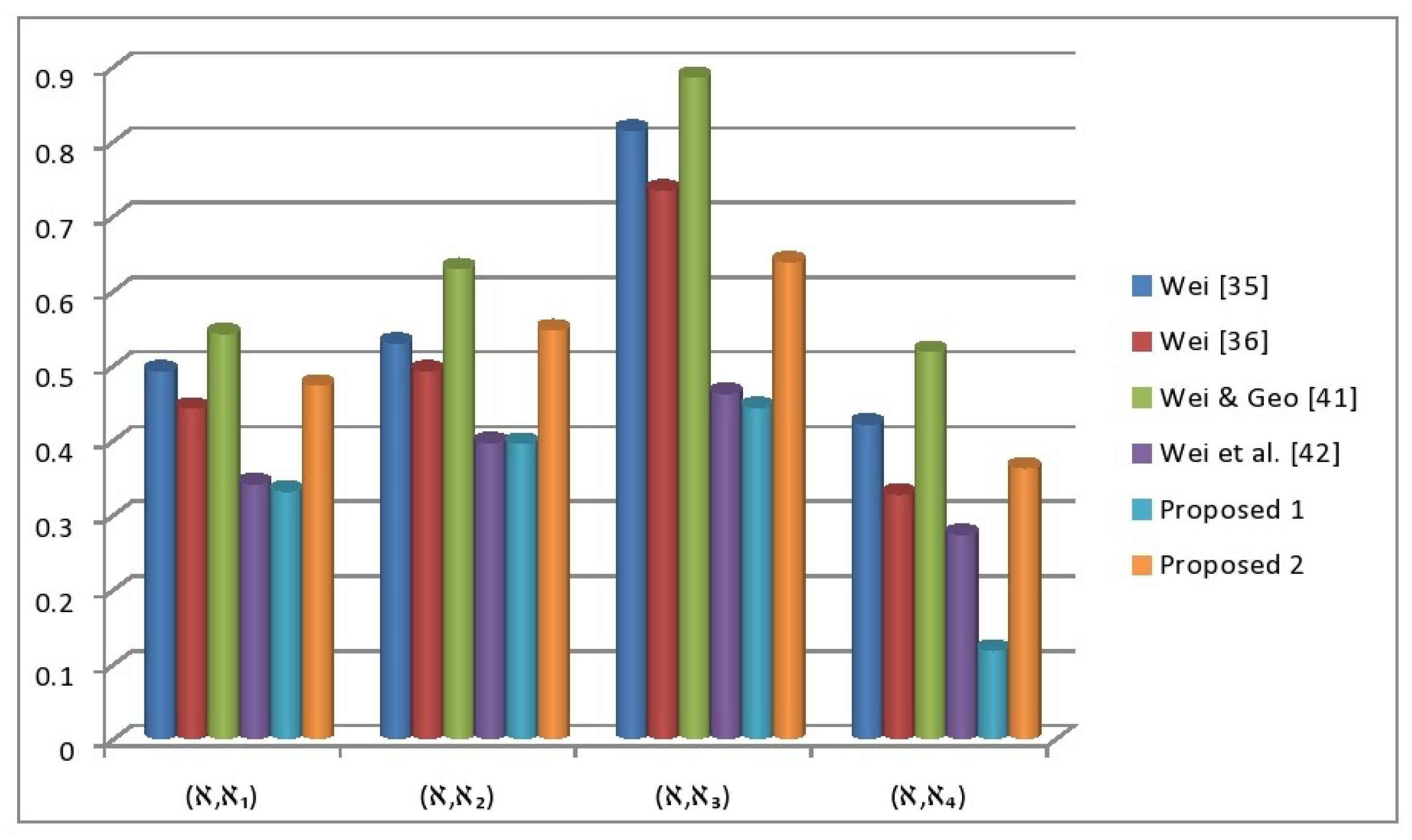
5. Comparative Study

The comparison of the developed measures with the other existing measures to examine the reliability and effectiveness of the explored measures. The established similarity measures are compared with the some other similarity measures based on PFS was established by Wei [39], cosine similarity measures based on PFS was established by Wei [40], dice similarity measures based on PFS was established by Wei and Gao [46], and similarity measures based on SFS was established by Wei et al. [45].
Example 2.
In this example, we choose the picture fuzzy types of information and examine the comparison of the defined measures with the existing measures. For this, we considered five different types of criteria i ( i = 1 , . . . , 5 ) with the weights are w = ( 0.20 , 0.12 , 0.10 , 0.33 , 0.25 ) T by the known alternative denoted by i ( 1 i 4 ) . Table 4 identify that the information about the unknown and known alternatives. For more information, we suggest the Example 1.
Step 1. Class about unknown and known FOFNs
The comparison of the established work with other existing work is discussed for Example 2, is express in Table 5. Graphical presentation is given in Figure 2.
Analyzing Table 5, it seems that the SM of ( , 3 ) is greatest among all other SMs.

Sensitivity Analysis

The SMs proposed in this article are generalization of existing SMs for SFSs, PyFSs, PFSs and IFSs. The following remarks show that the SMs defined in Equations (13)–(22) are generalization of SMs for SFSs, PyFSs, PFSs and IFSs. From Table 4 and Table 5, we obtain that the established measures on the based of FOFS is more reliable and more general than the existing concepts due to its limit condition. When, we choose the fractional orthotriple fuzzy types of information, the existing drawbacks is not able to solve it, but when we choose the existing types of data like in Example 2, then the developed method can be solve it easily.
Remark 5.
In Definition (18), if
We put f = 2 , then Equation (14) reduced to WSM of SFS such as;
W S F C 1 , = 1 m i = 1 m ω i σ 2 ( i ) σ 2 ( i ) + η 2 ( i ) η 2 ( i ) + υ 2 ( i ) υ 2 ( i ) σ 4 ( i ) + η 4 ( i ) + υ 4 ( i ) σ 4 ( i ) + η 4 ( i ) + υ 2 ( i )
We put f = 2 and η = 0 , then Equation (14) reduces to WSM of PyFS such as;
W P y F C 1 , = 1 m i = 1 m ω i σ 2 ( i ) σ 2 ( i ) + υ 2 ( i ) υ 2 ( i ) σ 4 ( i ) + υ 4 ( i ) σ 4 ( i ) + υ 4 ( i )
We put f = 1 , then Equation (14) reduces to WSM of PFS such as:
W P F C 1 , = 1 m i = 1 m ω i σ ( i ) σ ( i ) + η ( i ) η ( i ) + υ ( i ) υ ( i ) σ 2 ( i ) + η 2 ( i ) + υ 2 ( i ) σ 2 ( i ) + η 2 ( i ) + υ 2 ( i )
We put f = 1 , and η = 0 , then Equation (14) reduces to WSM of IFS such as:
W I F C 1 , = 1 m i = 1 m ω i σ ( i ) σ ( i ) + υ ( i ) υ ( i ) σ 4 ( i ) + υ 4 ( i ) σ 4 ( i ) + υ 2 ( i )
Remark 6.
In Definition (20), if
We put f = 2 , then Equation (17) reduces to WSM of SFS such that
W S F C S 1 ( , ) = 1 m i = 1 m ω i cos π 2 σ 2 ( i ) σ 2 ( i ) η 2 ( i ) η 2 ( i ) υ 2 ( i ) υ 2 ( i )
We put f = 2 and η = 0 , then Equation (17) reduces to WSM of PyFS such that
W P y F C S 1 ( , ) = 1 m i = 1 m ω i cos π 2 ( | σ 2 ( i ) σ 2 ( i ) | | υ 2 ( i ) υ 2 ( i ) | )
We put f = 1 , then Equation (17) reduces to WSM of PFS such that
W P F C S 1 ( , ) = 1 m i = 1 m ω i cos π 2 σ ( i ) σ ( i ) η ( i ) η ( i ) υ ( i ) υ ( i )
We put f = 1 and η = 0 , then Equation (17) reduces to WSM of IFS such that
W I F C S 1 ( , ) = 1 m i = 1 m ω i cos π 2 σ ( i ) σ ( i ) υ ( i ) υ ( i )
Remark 7.
In the Definition (22), if
We put f = 2 , then Equation (22) reduces to WSM of SFS such that
W S F C T 1 ( , ) = 1 m i = 1 m ω i cot π 4 + π 4 σ 2 ( i ) σ 2 ( i ) η 2 ( i ) η 2 ( i ) υ 2 ( i ) υ 2 ( i )
We put f = 2 and η = 0 , then Equation (22) reduces to WSM of PyFS such that
W P y F C T 1 ( , ) = 1 m i = 1 m ω i cot π 4 + π 4 ( | σ 2 ( i ) σ 2 ( i ) | | υ 2 ( i ) υ 2 ( i ) | )
∘ We put f = 1 , then Equation (17) reduces to WSM of PFS such that
W P F C T 1 ( , ) = 1 m i = 1 m ω i cot π 4 + π 4 σ ( i ) σ ( i ) η ( i ) η ( i ) υ ( i ) υ ( i )
We put f = 1 and η = 0 , then Equation (22) reduces to WSM of IFS such that
W I F C T 1 ( , ) = 1 m i = 1 m ω i cot π 4 + π 4 σ ( i ) σ ( i ) υ ( i ) υ ( i )

6. Conclusions

Similarity measures of FSs are important topic in fuzzy mathematics and have gained some serious attention from researchers due to its successful applications in real life. In this article, we discussed the basic notions of IFSs, PyFSs, PFSs, SFSs and FOFSs are analyzed along with their SMs. We observed that the concept of SM for FOFS has not define in past. Therefore, we defined concept of SM for the FOFSs. Some new SMs and weighted SMs (WSMs) have been developed so far in Section 3. The characteristics of these similarity measures have been investigated and some results are proved. These SMs resolve the limitations of some of the current SMs of the spherical fuzzy sets. Further, the developed SMs and WSMs are applied to pattern recognition problem of crane accident. In addition, the proposed approach is compared to the existing approaches and discussed the conditions under which the proposed approach reduced to existing approaches. The sensitive analysis of proposed new work over the existing work have also been studied. In future, the proposed results can be utilized in DM problem and can be extended to (1) generalized dice similarity measures for picture fuzzy sets and their applications; (2) similarity and inclusion measures between type-2 fuzzy sets with an application to clustering; (3) MAGDM problem with complex q-Rung orthopair linguistic information based on Heronian mean operators; (4) covering-based Spherical fuzzy Rough set model Hybrid with TOPSIS for MADM; (5) some distance measures of complex PyFSs and their applications in pattern recognition.

Author Contributions

All authors are equally contributed to this paper. All authors have read and agreed to the published version of the manuscript.

Funding

This research was funded by Deanship of Scientific Research at Umm Al-Qura University grant number 19-SCI-101-0056 and APC was funded by grant number 19-SCI-101-0056.

Acknowledgments

The authors would like to thank the Deanship of Scientific Research at Umm Al-Qura University for supporting this work by grant number 19-SCI-101-0056.

Conflicts of Interest

The authors declare no conflict of interest.

References

  1. Zadeh, L.A. Fuzzy sets. Inf. Control 1965, 8, 338–353. [Google Scholar] [CrossRef] [Green Version]
  2. Atanassov, K.T. Intuitionistic fuzzy sets. Fuzzy Sets Syst. 1986, 20, 87–96. [Google Scholar] [CrossRef]
  3. Yager, R.R. Pythagorean fuzzy subsets. In Proceedings of the 2013 Joint IFSA World Congress and NAFIPS Annual Meeting (IFSA/NAFIPS), Edmonton, AB, Canada, 24–28 June 2013; pp. 57–61. [Google Scholar]
  4. Yager, R.R.; Abbasov, A.M. Pythagorean membership grades, complex numbers and decision making. Int. J. Intell. Syst. 2013, 28, 436–452. [Google Scholar] [CrossRef]
  5. Asiain, M.J.; Bustince, H.; Mesiar, R.; Kolesárová, A.; Takáč, Z. Negations with respect to admissible orders in the interval-valued fuzzy set theory. IEEE Trans. Fuzzy Syst. 2018, 26, 556–568. [Google Scholar] [CrossRef]
  6. Mahmood, T.; Liu, P.; Ye, J.; Khan, Q. Several hybrid aggregation operators for triangular intuitionistic fuzzy set and their application in multi-criteria decision making. Granul. Comput. 2018, 3, 153–168. [Google Scholar] [CrossRef]
  7. Li, H. 3D distances of intuitionistic fuzzy sets based on hesitating index. In Proceedings of the Chinese Control and Decision Conference (CCDC), Liaoning, China, 9–11 June 2018; pp. 2514–2518. [Google Scholar]
  8. Peng, X.; Yang, Y. Some results for Pythagorean fuzzy sets. Int. J. Intell. Syst. 2015, 30, 1133–1160. [Google Scholar] [CrossRef]
  9. Garg, H. A new generalized Pythagorean fuzzy information aggregation using Einstein operations and its application to decision making. Int. J. Intell. Syst. 2016, 31, 886–920. [Google Scholar] [CrossRef]
  10. Wei, G.; Lu, M. Pythagorean fuzzy Maclaurin symmetric mean operators in multiple attribute decision making. Int. J. Intell. Syst. 2018, 33, 1043–1070. [Google Scholar] [CrossRef]
  11. Wei, G.; Lu, M. Pythagorean Hesitant Fuzzy Hamacher Aggregation Operators in Multiple-Attribute Decision Making. J. Intell. Syst. 2017, 28, 756–776. [Google Scholar] [CrossRef]
  12. Lu, M.; Wei, G.; Alsaadi, F.E.; Hayat, T.; Alsaedi, A. Hesitant Pythagorean fuzzy hamacher aggregation operators and their application to multiple attribute decision making. J. Intell. Fuzzy Syst. 2017, 33, 1105–1117. [Google Scholar] [CrossRef]
  13. Cuong, B.C. Picture fuzzy sets. J. Comput. Sci. Cybern. 2014, 30, 409. [Google Scholar]
  14. Akram, M.; Bashir, A.; Garg, H. Decision-making model under complex picture fuzzy Hamacher aggregation operators. Comput. Appl. Math. 2020, 39, 1–38. [Google Scholar] [CrossRef]
  15. Khalil, A.M.; Li, S.G.; Garg, H.; Li, H.; Ma, S. New operations on interval-valued picture fuzzy set, interval-valued picture fuzzy soft set and their applications. IEEE Access 2019, 7, 51236–51253. [Google Scholar] [CrossRef]
  16. Garg, H. Some picture fuzzy aggregation operators and their applications to multicriteria decision-making. Arab. J. Sci. Eng. 2017, 42, 5275–5290. [Google Scholar] [CrossRef]
  17. Lin, M.; Huang, C.; Xu, Z. MULTIMOORA based MCDM model for site selection of car sharing station under picture fuzzy environment. Sustain. Cities Soc. 2020, 53, 101873. [Google Scholar] [CrossRef]
  18. Liu, P.; Munir, M.; Mahmood, T.; Ullah, K. Some similarity measures for interval-valued picture fuzzy sets and their applications in decision making. Information 2019, 10, 369. [Google Scholar] [CrossRef] [Green Version]
  19. Wei, G. Picture fuzzy Hamacher aggregation operators and their application to multiple attribute decision making. Fundam. Inform. 2018, 157, 271–320. [Google Scholar] [CrossRef]
  20. Singh, P. Correlation coefficients for picture fuzzy sets. J. Intell. Fuzzy Syst. 2015, 28, 591–604. [Google Scholar] [CrossRef]
  21. Mahmood, T.; Ullah, K.; Khan, Q.; Jan, N. An approach toward decision-making and medical diagnosis problems using the concept of spherical fuzzy sets. Neural Comput. Appl. 2019, 31, 7041–7053. [Google Scholar] [CrossRef]
  22. Peng, Y.F.; Chiu, C.H.; Tsai, W.R.; Chou, M.H. Design of an omni-directional spherical robot: Using fuzzy control. In Proceedings of the International Multiconference of Engineers and Computer Scientists, Hong Kong, China, 13–15 March 2019; Volume 1, pp. 18–20. [Google Scholar]
  23. Ashraf, S.; Abdullah, S.; Aslam, M.; Qiyas, M.; Kutbi, M.A. Spherical fuzzy sets and its representation of spherical fuzzy t-norms and t-conorms. J. Intell. Fuzzy Syst. 2019, 36, 6089–6102. [Google Scholar] [CrossRef]
  24. Zeng, S.; Hussain, A.; Mahmood, T.; Irfan Ali, M.; Ashraf, S.; Munir, M. Covering-Based Spherical Fuzzy Rough Set Model Hybrid with TOPSIS for Multi-Attribute Decision-Making. Symmetry 2019, 11, 547. [Google Scholar] [CrossRef] [Green Version]
  25. Liu, P.; Khan, Q.; Mahmood, T.; Hassan, N. T-spherical fuzzy power Muirhead mean operator based on novel operational laws and their application in multi-attribute group decision making. IEEE Access 2019, 7, 22613–22632. [Google Scholar] [CrossRef]
  26. Ullah, K.; Hassan, N.; Mahmood, T.; Jan, N.; Hassan, M. Evaluation of investment policy based on multi-attribute decision-making using interval valued T-spherical fuzzy aggregation operators. Symmetry 2019, 11, 357. [Google Scholar] [CrossRef] [Green Version]
  27. Zeng, S.; Garg, H.; Munir, M.; Mahmood, T.; Hussain, A. A Multi-Attribute Decision Making Process with Immediate Probabilistic Interactive Averaging Aggregation Operators of TSpherical Fuzzy Sets and Its Application in the Selection of Solar Cells. Energies 2019, 12, 4436. [Google Scholar] [CrossRef] [Green Version]
  28. Garg, H.; Munir, M.; Ullah, K.; Mahmood, T.; Jan, N. Algorithm for T-spherical fuzzy multiattribute decision making based on improved interactive aggregation operators. Symmetry 2018, 10, 670. [Google Scholar] [CrossRef] [Green Version]
  29. Dengfeng, L.; Chuntian, C. New SMs of intuitionistic fuzzy sets and application to pattern recognitions. Pattern Recognit. Lett. 2002, 23, 221–225. [Google Scholar] [CrossRef]
  30. Hung, W.L.; Yang, M.S. SMs of intuitionistic fuzzy sets based on Hausdorff distance. Pattern Recognit. Lett. 2004, 25, 1603–1611. [Google Scholar] [CrossRef]
  31. Vlachos, I.K.; Sergiadis, G.D. Intuitionistic fuzzy information–applications to pattern recognition. Pattern Recognit. Lett. 2007, 28, 197–206. [Google Scholar] [CrossRef]
  32. Son, L.H.; Phong, P.H. On the performance evaluation of intuitionistic vector SMs for medical diagnosis 1. J. Intell. Fuzzy Syst. 2016, 31, 1597–1608. [Google Scholar] [CrossRef]
  33. Miaoying, T. A new fuzzy SM based on cotangent function for medical diagnosis. Adv. Model. Optim. 2013, 15, 151–156. [Google Scholar]
  34. Xia, M.; Xu, Z. Some new SMs for intuitionistic fuzzy values and their application in group decision making. J. Syst. Syst. Eng. 2010, 19, 430–452. [Google Scholar] [CrossRef]
  35. Yang, M.S.; Lin, D.C. On similarity and inclusion measures between type-2 fuzzy sets with an application to clustering. Comput. Math. Appl. 2009, 57, 896–907. [Google Scholar] [CrossRef] [Green Version]
  36. Ye, J. Cosine SMs for intuitionistic fuzzy sets and their applications. Math. Comput. Model. 2011, 53, 91–97. [Google Scholar] [CrossRef]
  37. Rajarajeswari, P.; Uma, N. Intuitionistic fuzzy multi SM based on cotangent function. Int. J. Eng. Res. Technol. 2013, 2, 1323–1329. [Google Scholar]
  38. Ye, J. SMs of intuitionistic fuzzy sets based on cosine function for the decision making of mechanical design schemes. J. Intell. Fuzzy Syst. 2016, 30, 151–158. [Google Scholar] [CrossRef]
  39. Wei, G. Some SMs for picture fuzzy sets and their applications. Iran. J. Fuzzy Syst. 2018, 15, 77–89. [Google Scholar]
  40. Wei, G. Some cosine SMs for picture fuzzy sets and their applications to strategic decision making. Informatica 2017, 28, 547–564. [Google Scholar] [CrossRef] [Green Version]
  41. Ahmad, Z.; Mahmood, T.; Saad, M.; Jan, N.; Ullah, K. SMs for picture hesitant fuzzy sets and their applications in pattern recognition. J. Prime Res. Math. 2019, 15, 81–100. [Google Scholar]
  42. Wei, G.; Wei, Y. SMs of Pythagorean fuzzy sets based on the cosine function and their applications. Int. J. Intell. Syst. 2018, 33, 634–652. [Google Scholar] [CrossRef]
  43. Ullah, K.; Mahmood, T.; Jan, N. SMs for T-spherical fuzzy sets with applications in pattern recognition. Symmetry 2018, 10, 193. [Google Scholar] [CrossRef] [Green Version]
  44. Abosuliman, S.S.; Abdullah, S.; Qiyas, M. Three-Way Decisions Making Using Covering Based Fractional Orthotriple Fuzzy Rough Set Model. Mathematics 2020, 8, 1121. [Google Scholar] [CrossRef]
  45. Wei, G.; Wang, J.; Lu, M.; Wu, J.; Wei, C. Similarity measures of spherical fuzzy sets based on cosine function and their applications. IEEE Access 2019, 7, 159069–159080. [Google Scholar] [CrossRef]
  46. Wei, G.; Gao, H. The generalized Dice similarity measures for picture fuzzy sets and their applications. Informatica 2018, 29, 107–124. [Google Scholar] [CrossRef] [Green Version]
Figure 1. Ranking of the alternatives.
Mathematics 08 01653 g001
Figure 2. Comparative Study of the alternatives.
Mathematics 08 01653 g002
Table 1. Data in the form of FOFNs.
1 2 3 4
1 0.39 , 0.65 , 0.81 ( 0.61 , 0.15 , 0.92 ) ( 0.83 , 0.57 , 0.35 ) ( 0.44 , 0.41 , 0.57 ) ( 0.93 , 0.07 , 0.29 )
2 ( 0.49 , 0.41 , 0.82 ) ( 0.36 , 0.54 , 0.74 ) ( 0.58 , 0.86 , 0.67 ) ( 0.93 , 0.33 , 0.69 ) ( 0.20 , 0.77 , 0.46 )
3 ( 0.53 , 0.47 , 0.91 ) ( 0.96 , 0.04 , 0.11 ) ( 0.43 , 0.58 , 0.70 ) ( 0.26 , 0.74 , 0.42 ) ( 0.56 , 0.32 , 0.73 )
4 ( 0.79 , 0.42 , 0.84 ) ( 0.47 , 0.73 , 0.82 ) ( 0.59 , 0.73 , 0.46 ) ( 0.43 , 0.51 , 0.81 ) ( 0.44 , 0.58 , 0.47 )
5 ( 0.91 , 0.52 , 0.09 ) ( 0.37 , 0.77 , 0.61 ) ( 0.45 , 0.72 , 0.35 ) ( 0.57 , 0.43 , 0.79 ) ( 0.55 , 0.67 , 0.91 )
Table 2. Similarity measures of i with .
SMs , 1 , 2 , 3 , 4
F O F C 1 , i 0.5826 ( 0.5219 ) ( 0.4964 ) ( 0.3672 )
F O F C S 1 , i ( 0.7183 ) ( 0.7251 ) ( 0.7125 ) ( 0.6689 )
F O F C S 2 , i ( 0.7927 ) ( 0.8428 ) ( 0.8214 ) ( 0.7615 )
F O F C T 1 , i ( 0.4825 ) ( 0.4163 ) ( 0.4416 ) ( 0.4042 )
F O F C T 2 , i ( 0.4721 ) ( 0.4478 ) ( 0.4171 ) ( 0.3752 )
Table 3. Weighted similarity measures of i with .
WSMs , 1 , 2 , 3 , 4
W F O F C 1 , i 0.6162 ( 0.4783 ) ( 0.5841 ) ( 0.3326 )
W F O F C S 1 , i ( 0.7367 ) ( 0.6946 ) ( 0.7559 ) ( 0.6689 )
W F O F C S 2 , i ( 0.8628 ) ( 0.8749 ) ( 0.8414 ) ( 0.8853 )
W F O F C T 1 , i ( 0.4924 ) ( 0.4332 ) ( 0.5163 ) ( 0.3947 )
W F O F C T 2 , i ( 0.5041 ) ( 0.4283 ) ( 0.4371 ) ( 0.3461 )
Table 4. Given data in the form of FOFNs.
1 2 3 4
1 0.33 , 0.29 , 0.25 ( 0.41 , 0.37 , 0.1 ) ( 0.60 , 0.19 , 0.11 ) ( 0.33 , 0.31 , 0.28 ) ( 0.43 , 0.38 , 0.13 )
2 ( 0.29 , 0.33 , 0.25 ) ( 0.39 , 0.33 , 0.14 ) ( 0.53 , 0.23 , 0.09 ) ( 0.32 , 0.36 , 0.21 ) ( 0.41 , 0.37 , 0.15 )
3 ( 0.31 , 0.28 , 0.28 ) ( 0.43 , 0.35 , 0.13 ) ( 0.57 , 0.25 , 0.05 ) ( 0.34 , 0.33 , 0.26 ) ( 0.33 , 0.23 , 0.17 )
4 ( 0.37 , 0.31 , 0.23 ) ( 0.40 , 0.37 , 0.17 ) ( 0.52 , 0.27 , 0.08 ) ( 0.37 , 0.29 , 0.22 ) ( 0.38 , 0.31 , 0.12 )
5 ( 0.32 , 0.33 , 0.31 ) ( 0.47 , 0.34 , 0.11 ) ( 0.51 , 0.31 , 0.04 ) ( 0.31 , 0.33 , 0.29 ) ( 0.42 , 0.37 , 0.14 )
Table 5. Comparison of the defined work with the existing drawbacks.
MethodsSimilarity MeasureRanking
Wei [39] S P F S ( , 1 ) = 0.492 , S P F S ( , 2 ) = 0.529
S P F S ( , 3 ) = 0.814 , S P F S ( , 4 ) = 0.421
3 2 1 4
Wei [40] S P F S ( , 1 ) = 0.442 , S P F S ( , 2 ) = 0.492
S P F S ( , 3 ) = 0.734 , S P F S ( , 4 ) = 0.327
3 2 1 4
Wei and Gao [46] S P F S ( , 1 ) = 0.542 , S P F S ( , 2 ) = 0.629
S P F S ( , 3 ) = 0.885 , S P F S ( , 4 ) = 0.518
3 2 1 4
Wei et al. [45] S P F S ( , 1 ) = 0.341 , S P F S ( , 2 ) = 0.396
S P F S ( , 3 ) = 0.462 , S P F S ( , 4 ) = 0.273
3 2 1 4
F O F C S 2 ( , i ) S P F S ( , 1 ) = 0.331 , S P F S ( , 2 ) = 0.395
S P F S ( , 3 ) = 0.443 , S P F S ( , 4 ) = 0.118
3 2 1 4
W F O F C S 2 ( , i ) S P F S ( , 1 ) = 0.473 , S P F S ( , 2 ) = 0.547
S P F S ( , 3 ) = 0.638 , S P F S ( , 4 ) = 0.362
3 2 1 4

