Free Interfaces at the Tips of the Cilia in the One-Dimensional Periciliary Layer

Department of Mathematics, King Mongkut’s Institute of Technology Ladkrabang, Bangkok 10520, Thailand
Mathematics 2020, 8(11), 1961; https://doi.org/10.3390/math8111961
Submission received: 18 October 2020
/
Revised: 29 October 2020
/
Accepted: 31 October 2020
/
Published: 5 November 2020
(This article belongs to the Section Computational and Applied Mathematics)
Abstract
:Cilia on the surface of ciliated cells in the respiratory system are organelles that beat forward and backward to generate metachronal waves to propel mucus out of lungs. The layer that contains the cilia, coating the interior epithelial surface of the bronchi and bronchiolesis, is called the periciliary layer (PCL). With fluid nourishment, cilia can move efficiently. The fluid in this region is named the PCL fluid and is considered to be an incompressible, viscous, Newtonian fluid. We propose there to be a free boundary at the tips of cilia underlining a gas phase while the cilia are moving forward. The Brinkman equation on a macroscopic scale, in which bundles of cilia are considered rather than individuals, with the Stefan condition was used in the PCL to determine the velocity of the PCL fluid and the height/shape of the free boundary. Regarding the numerical methods, the boundary immobilization technique was applied to immobilize the moving boundaries using coordinate transformation (working with a fixed domain). A finite element method was employed to discretize the mathematical model and a finite difference approach was applied to the Stefan problem to determine the free interface. In this study, an effective stroke is assumed to start when the cilia make a 140 angle to the horizontal plane and the velocitiesof cilia increase until the cilia are perpendicular to the horizontal plane. Then, the velocities of the cilia decrease until the cilia make a angle with the horizontal plane. From the numerical results, we can see that although the velocities of the cilia increase and then decrease, the free interface at the tips of the cilia continues increasing for the full forward phase. The numerical results are verified and compared with an exact solution and experimental data from the literature. Regarding the fixed boundary, the numerical results converge to the exact solution. Regarding the free interface, the numerical solutions were compared with the average height of the PCL in non-cystic fibrosis (CF) human tissues and were in excellent agreement. This research also proposes possible values of parameters in the mathematical model in order to determine the free interface. Applications of these fluid flows include animal hair, fibers and filter pads, and rice fields.
1. Introduction
Breathing in polluted particles, such as dust and bacteria, is often unavoidable for people. At the same time, the innate immune system plays an important role in protecting the body by secreting mucus from goblet cells lining the airway epithelium to trap particles and remove them through the beat cycle of the cilia. This system is called muco-ciliary transport and has been studied by several authors [1,2,3,4,5,6,7,8,9]. Muco-ciliary clearance is fundamental for the health of the human respiratory system. Muco-ciliary dysfunction causes chronic airway diseases in humans, such as cystic fibrosis, primary ciliary dyskinesia, asthma, and chronic bronchitis. Moreover, deficient mucus clearance is not completely understood. For example, cystic fibrosis is a disease which depletes the volume of fluid or the height of the fluid in the respiratory system. Further investigations are vitally needed to investigate the effect of changing the volume or height of the fluid to improve muco-ciliary transport. In the respiratory system, cilia are contained in a layer called the periciliary layer (PCL), which consists of PCL fluid. Above the PCL is a layer of viscoelastic mucus. Figure 1 shows a portion of the patchwork of muco-ciliary clearance in the respiratory system.
At the epithelial cells, there are goblet cells, scattered among ciliated cells, which secrete mucus, a viscous fluid, to trap particulate matter and micro-organisms. This clearance prevents them from reaching the lungs. After this, the mucus forms a mucus blanket floating on a lower viscous fluid layer, the PCL, which contains the cilia covering the surface of the epithelial cells. Cilia beat back and forth about 12 times per second to propel mucus at 1 millimeter per minute [10], beating along the same plane without sweeping sideways during the effective stroke [11,12]. Above the mucous layer is air moving in and out of the human body. Because the height of the PCL contributes a significant role in the muco-ciliary clearance system, we first focus on the free surface or the height of the PCL fluid at the tips of cilia.
Several studies modeled cilia movement in both experimentally and numerically. For example, Quek et al. [13] simulated the ciliary flow in a three-dimensional domain using the immersed boundary method. They concluded that the stiffness and the cilia density effected the slip velocity at the tips of cilia. Cilia in both high and low densities had a low slip velocity and the wave propagation was not supported by long stiff cilia. Sears et al. [9] used video microscopy to record ciliary motion. They converted planar ciliary motions into an empirical quantitative model, which was easy to use for examining ciliary function. If the tip of a cilium was modeled to penetrate the mucous layer, an integral equation could be used to express the mean velocity field in the mucous layer involving the tips of the cilia [2]. Fine-tuned methods of this kind can be found in [14,15,16,17].
Cilia were detected by several researchers. Some considered cilia and flagella to have the bending properties of an axoneme [18,19,20]. Den Toonder and Onck [21] studied and reviewed artificial cilia in many aspects, such as the bead-spring model for artificial cilia, a superparamagnetic filament for fluid transport, modeling the interaction of active cilia with species, electrostatic artificial cilia, microwalkers, artificial flagellar microswimmers, fluid manipulation by artificial cilia, and the measurement of fluid flow generated by artificial cilia.
Because the problem considered in this study is the one-dimensional prototype problem of finding the free surface at the tips of the cilia while the cilia move and drive the PCL fluid, instead of typical pressure gradient doing so, we first assume there to be a fluid–gas phase at the free surface. Because of the inference of the phases, the height of our domain, in this study, is proposed to change according to the angle that the cilia make with the horizontal plane, as shown in Figure 2. Figure 2 demonstrates the domain when (left figure) the cilia are perpendicular and (right figure) make a angle with the horizontal plane. The variable is the length of a cilium and z is the axis. The heights of the domains in both figures depend on the tips of the cilia and the free surface that occurs at the distal ends of the cilia. To model the problem, since the PCL contains both PCL fluid and solid phases, i.e., cilia, it can be formed as a porous medium, see Figure 2. In this study, we consider the movement of bundles of cilia effecting the PCL fluid. Therefore, we use the Brinkman equation to predict the velocity of the PCL fluid in the porous region. Numerical and analytical studies can be found in the literature that focus on the fluid flow through the domain using the Brinkman equations [22,23,24,25,26]. For example, Morandotti [25] proved the existence and the uniqueness of the Brinkman model for the movement of a self-propelled microswimmer. Skrzypacz and Wei [26] proved the existence and uniqueness of a weak solution of the nonlinear Brinkman–Forchheimer–Darcy equation for the flow in chemical reactors of the packed-bed type. Liou and Lu [23] applied the Brinkman equation to flow over rough walls using the volume-averaging method. Cortez et al. [24] found the exact solution of the three-dimensional Brinkman equation where the flow was driven by regularized forces. Shavit et al. [22] suggested a modified Brinkman equation was a good fit with a free flow problem.
There are a variety of numerical methods that study free boundary problems, such as the level-set method (LSM), the immersed boundary method, the simple line interface calculation (SLIC), the flux line-segment model for advection and interface reconstruction (FLAIR), and the volume-of-fluid method (VOF). For example, Ashgriz and Poo [27] initially developed the FLAIR method to predict the free surfaces of problems, originally taking the idea from Youngs [28] of using a sloped line in the interface reconstruction. Hirt and Nichols [29] established the volume-of-fluid method to extract the interface. Mashayek and Ashgriz [30] claimed that the volume-of-fluid method could handle large surface deformations. Although, there are several free boundary methods, to author’s knowledge, there have been no studies conducted on the cilia movement in the PCL with a free boundary method. Because we assume there to be a fluid–gas phase at the free interface, we apply the Stefan problem [31,32] at the tips of cilia where the free surface is changed with respect to the angle , instead of time t. Because cilia tips touch the mucous layer only on the effective stroke [33], our objective was to investigate the free interface at the tips of the cilia for the forward stroke, provide feasible numerical results, and compare the results with the experimental data available in literature. The free interface obtained in this work becomes the lower boundary of the mucus. Our latter goal was to study changes in the sensitivity of the free interface of the PCL when the free surface of the mucus changes. If it is responsive, this indicates that we have to repeat our protocol to find the velocity of the mucus.
The mathematical model is provided in Section 2. To avoid the computational grid adjustment for each angle, we applied the boundary immobilization technique to the model in Section 3. Model discretization is presented in Section 4. The validation of the numerical results and numerical solutions is provided in Section 5 and Section 6, respectively. The conclusion is drawn in Section 7.
2. Mathematical Model
In order to consider the motion of cilia collectively, rather than that of a single cilium, the governing equation employed in this work is the Brinkman equation on the macroscopic scale. They were upscaled using the hybrid mixture theory (HMT) [34,35,36,37], i.e., by applying the averaging theorem to average the microscale field equations to obtain the macroscale equations. In this work, we consider the model in steady state. That is [37,38]
where is the porosity; and are the velocities of the liquid and solid phases, respectively; ; is a dynamic viscosity; is the inverse of the permeability tensor; p is pressure; is fluid density; is gravity; is the material time derivative of the porosity with respect to the solid phase, . Let
Figure 3 illustrates the fluid flow at the tips of the cilia, where the domain containing cilia is considered as a porous medium. In this work, we assume that the pressure gradient is zero in the z direction and a constant in the x direction. The velocity and the other variables depend on the z direction. Substituting (5) into (4), we obtain (4) in one-dimensional space z as
For the boundary condition between the free fluid and porous medium interface, we were motivated by [39], where they used Beaver and Joseph boundary condition at the top of a porous region. We then use the boundary condition
where r is a continuous function depending on the axis and the angle ; q is a function of the angle at the free surface; and is a constant. We also employ the Stefan problem [31] at the free-fluid/porous-medium interface with the rate of change of the interface with respect to the angle . That is
with the initial condition
where c is a constant and is the initial angle.
3. Boundary Immobilization Technique
Because of the free boundary at the free-fluid/porous-medium interface, we employ a boundary immobilization technique [32] to the problem. Define the spatial coordinate transformation as
to fix the moving surface to a fixed coordinate system in space, where is the dimensionless variable, z is the spatial coordinate, and is the function of the angle at the free-fluid/porous-medium interface. Therefore, at , . Thus,
Applying partial differential relations to the velocity , we have
Similarly, the boundary and initial conditions become
To calculate the numerical results, model discretization is provided in the next section.
4. Model Discretization
In order to find the numerical solutions, the discretization of the Brinkman equation is provided in this section. We apply a finite element method to the system of Equations (14)–(18). Using the Galerkin finite element method, where the test function w comes from a chosen trial function [40], the weak formulation of the one-dimensional governing Equation (14) is to find , such that
where is our computational domain; is the Hilbert space; and is the test function. The n element discretization of (19) is
Define the finite-dimensional subspaces of the Hilbert space as follows
where is a single line segment of the domain. The approximate solution is
where is the vector of the velocity; is called a basis function; is its vector form; and the integer M is determined by the interpolation function. For a linear shape function, . In this study, we use linear isoparametric element,
with
where is the variable in natural coordinates as shown in Figure 4, which illustrates the mapping between the physical () and natural () coordinate systems using the shape functions (23) and the interpolation (24). This is effective for numerical integration because the linear element is normalized between and 1 in the natural coordinate system. Therefore,
where is the distance between adjacent points of a uniform mesh.
Hence, the vector of the velocity and the vector form of the basis function are
respectively. Substituting the vector form of the basis functions, in (26) into w in (20), and the approximate velocity in (22) into (20), we obtain the element matrix form of (20), which is
where the element matrices, in the natural coordinate, are
where the variable is the Jacobian, and
is the vector of the solid velocity in each element. After assembling the element matrices, we have the global matrix form,
where we use the same notation for both element and global vectors of the velocities for the sake of notation simplicity and the boundary term in (20) is added into the last component of the vector . Let
Because the velocity is zero at the bottom of the domain,
Since and at ,
Therefore,
where the second and third equalities come from (15) and (32), respectively. In this study, we employ the porosity and the velocity of cilia from [41], where they obtained the solid velocities from [9], which are the eighth-order polynomial functions as shown in Table 1 in [41]. Therefore,
and
where as shown in Figure 2. To discretize (17), we first change the variable q to be u using (32) and find its derivative with respect to . That is
Substituting (40) into (17), we obtain
A suitable discretization formula of (41) is [32]
where u at an initial angle is
where is the difference between two adjacent angles and N is the number of nodes of the numerical porous-medium domain. The validation of the numerical solutions and numerical results are presented in the next sections.
5. Numerical Validation
The numerical result of the discretized model is validated in this section. The exact solution of (14) is provided in [42] with a linear velocity of cilia, i.e., , and a fixed boundary conditions and , which is
where
The values of variables are , and , where and are set to be the values that the cilia are perpendicular to the horizontal plane. Figure 5 shows the exact and numerical solutions with , and 400 elements. The norm errors are presents in Table 1. They illustrate that the errors decrease when the number of elements increases, showing the convergence of the numerical results to the exact solution. Notice that the velocity rapidly changes at the upper part of the domain, which is close to . The numerical result is different from the analytical result, but the difference is not observable from the graph when the number of elements is 400. This example problem is well posed [38] and is independent of time, so the numerical results were expected to be very accurate.
6. Numerical Results
The velocities of the PCL fluid due to the forward stroke of the cilia are illustrated in this section. We assume that the cilia start at [9] and move forward with a decreasing angle, and then the cilia stop at . In this study, we calculate the PCL velocity when the angle decreases by 10. The velocities of the cilia, produced from data presented in [9], at each angle are shown in Table 1 in [41] which are plotted in Figure 5 in [41]. In this work, we arrange the velocities of the cilia at the angles to equal , respectively. To find the numerical results of the Brinkman equation, the initial velocity is assumed to occur at , which is defined to be an increasing function from 0 to a value which is less than m/s along the length of cilia.
We place the initial velocity in (42) and then calculate . Then, u at the angle is placed in (27). After assembling the element matrix, we obtain the velocity of the PCL fluid. Then, it becomes an initial velocity in (42). The iterative process is continued until we obtain the velocity of the PCL fluid for every angle .
The values of variables used in the program are the same as in Section 5, i.e., g/(m·s), g/, g/(). Regarding the other variables, the gravity m/s, , , where is the greatest length of cilia; is the maximum velocity of the cilia; and , where is the greatest vertical length when cilia make an angle with the horizontal plane. Because of the dimensionless coordinate, the values of are less than 1 and change depending on the angle . The values of permeability and the porosity were obtained from [41,43], respectively. Although Chamsri and Bennethum [43] found the permeability in a three-dimensional domain, in this work, we only adopt the permeability in the x direction, which is in [43]. This is because from Figure 13 in [41], the velocity in the x direction affects the average velocity of all directions the most, which has an essential role in the fluid flow above the cilia. Moreover, the diagonal element of the permeability highly influences the fluid flow.
With 200 elements, Figure 6 shows the velocities of the PCL fluid from the angle to . Notice that the velocities of the PCL fluid increase when the angles decreases. Figure 7 shows the velocities of the PCL fluid from the angle to . In this forward movement, the velocities of the cilia are slowing. Therefore, the velocities of the PCL fluid decrease as the angles decrease. Figure 8 shows the combination of the velocities of the PCL fluid in Figure 6 and Figure 7. This illustrates that the velocities increase until the angle, then they decrease from the to angles.
Figure 9 illustrates the average velocity of the PCL fluid for each angle . From left to right on the axis, the angle starts at and the angle decreases by 10 until , which is the full forward phase of cilia movement. Notice that although the highest velocity of the cilia is assumed to be at , the maximum velocity of the PCL fluid occurs at , which is the next angle from the angle that provides the highest velocity for the effective stroke of the cilia. The mean velocities of the first, 140–90, and second, 90–40, half of the forward stroke are m/s and m/s, respectively. The total average of the full effective stroke is 29.5866. The mean velocities are similar to the velocity of mucus provided in [44], i.e., m/s.
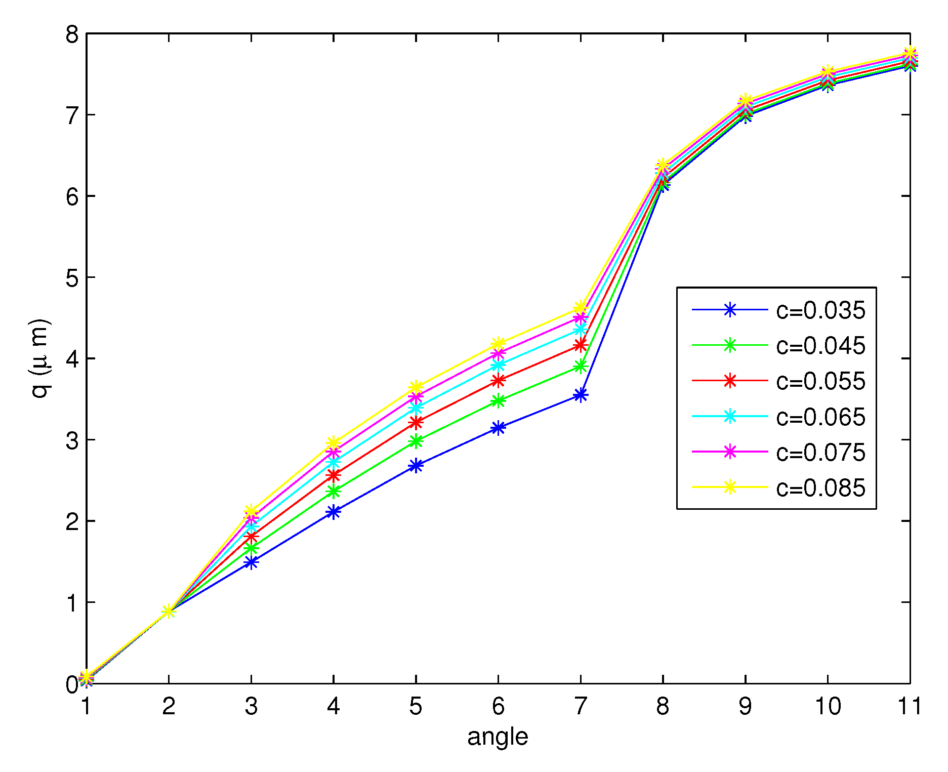
Figure 10 shows the free surface, q values, for the forward stroke at the tips of the cilia from the to angle. Although the angle becomes smaller, the free surface exhibits an increasing behavior. The numerical results are compared with the results in [45]. They measured the height of the PCL in human lower airway biopsies and in mice. The average height of the PCL in non-cystic fibrosis (CF) tissues was m, and in CF tissue, it was m. In mice, the non-CF PCL height was m and the CF height was m. They stated that the PCL fluid was reduced in patients with cystic fibrosis (CF). From Figure 10, we can see that the average of the free surface is , which is close to the height of the PCL in non-CF human tissues. Figure 11 and Figure 12 present the free surfaces for different variables r, which are and , respectively, with values of , where the angles are the same as those shown in Figure 10. The shapes of the free surfaces for different functions r are different but they are increasing functions of the angle for the forward stroke, and for each r, they have the same shape for different values c. The height of the free surface moves up when the initial values c increase.
7. Conclusions
We determine the free surface at the tips of the cilia due to the movement of cilia using the Brinkman equation on a macroscopic scale with the Stefan problem. In this work, we consider the free boundary between the phases, which moves with the change in the angle rather than time. We summarize the process and the results as follows.
- To avoid the numerical grid adjustment for every change in the the angle , we adopted the boundary immobilization technique to the mathematical model;
- The one-dimensional isotropic finite element method was applied to the Brinkman equation and a finite different scheme was employed to the Stefan problem to calculate the numerical solutions;
- The numerical results were verified by comparing them with an exact solution with a fixed boundary condition at when . The results converge to the exact solution, where the -norm errors are provided in Table 1;
- The numerical results of each angle are provided in Figure 6, Figure 7 and Figure 8 for the forward stroke from the angles to . Even if the velocity of the cilia is highest at (Figure 5 in [41]), the highest velocity of the PCL fluid is found at . That is, the velocities of the PCL fluid increase from the starting angle and decrease from the angles to ;
- The free surfaces due to the movement of cilia are shown in Figure 10, Figure 11 and Figure 12. We discovered that the height of the surface increases for the full forward stroke although the velocities of the PCL fluid increase in the first half of the effective stroke and decrease for the second half. Moreover, we found that the initial value c does not change the shape of the free surface, but the different functions r cause the change in the shape of the surface as illustrated in Figure 11 and Figure 12;
- To the author’s knowledge, no experimental data in the literature provide the shape of the free surface, only the average value is given. The numerical results were compared with the available experimental data. For the non-CF tissues, the average heights of the PCL from our results and the experimental data were and m, respectively. The difference between and is , which is small. This is one of the justifications that shows that our mathematical model is suitable for this problem.
Even though the mathematical model was developed in [32,37,38], in this study, we determined the free interfaces at the tips of cilia during the full forward stroke. From this, we hope to be able to further assess the natural velocity of mucus in future work. This study is a benchmark in terms of assessing the height and shape of the free boundary at the tips of cilia. In forthcoming work, we hope to determine the free boundary of the mucous layer, in which the result from this study will become the lower boundary of the mucous region. Consequently, we hope to extend the problem into the two- and then three-dimensional domains.
Funding
This research was supported by a grant from the Thailand Research Fund (TRF Fund).
Acknowledgments
The author would like to thank Lynn Schreyer for always giving good advice and nice support.
Conflicts of Interest
The authors declare no conflict of interest.
References
- Blake, J.R.; Winet, H. On the Mechanics of muco-ciliary transport. Biorheology 1980, 17, 125–134. [Google Scholar] [CrossRef]
- Fulford, G.R.; Blake, J.R. Muco-ciliary Transport in the Lung. J. Theor. Biol. 1986, 121, 381–402. [Google Scholar] [CrossRef]
- Sleigh, M.A. Adaptations of Ciliary Systems for the Propulsion of Water and Mucus. Comp. Biochem. Physiol. 1989, 94A, 359–364. [Google Scholar] [CrossRef]
- Hofmann, W.; Asgharian, B. Comparison of Mucociliary Clearance Velocities in Human and Rat Lungs for Extrapolation Modeling. Ann. Occup. Hyg. 2002, 46 (Suppl. 1), 323–325. [Google Scholar]
- Smith, D.J.; Gaffney, E.A.; Blake, J.R. A Viscoelastic Traction Layer Model of Muco-Ciliary Transport. Bull. Math. Biol. 2007, 69, 289–327. [Google Scholar] [CrossRef] [Green Version]
- Smith, D.J.; Gaffney, E.A.; Blake, J.R. Modelling Mucociliary Clearance. Respir. Physiol. Neurobiol. 2008, 163, 178–188. [Google Scholar] [CrossRef] [PubMed] [Green Version]
- Sears, P.R.; Davis, W.; Chua, M.; Sheehan, K. Mucociliary Interactions and Mucus Dynamics in Ciliated Human Bronchial Epithelial Cell Cultures. Am. J. Physiol. Lung Cell. Mol. Physiol. 2010, 301, L181–L186. [Google Scholar] [CrossRef] [PubMed] [Green Version]
- Lee, W.L.; Jayathilake, P.G.; Tan, Z.; Le, D.V.; Lee, H.P.; Khoo, B.C. Muco-Ciliary Transport: Effect of Mucus Viscosity, Cilia Beat Frequency and Cilia Density. Comput. Fluids 2011, 49, 214–221. [Google Scholar] [CrossRef]
- Sears, P.R.; Thompson, K.; Knowles, M.R.; Davis, C.W. Human Airway Ciliary Dynamics. Am. J. Physiol. Lung Cell. Mol. Physiol. 2012, 304, L170–L183. [Google Scholar] [CrossRef] [PubMed] [Green Version]
- Brawley, W. Health Check: What You Need to Know about Mucus and Phlegm. Available online: http://theconversation.com/health-check-what-you-need-to-know-about-mucus-and-phlegm-33192 (accessed on 5 July 2017).
- Chilvers, M.; O’Callaghan, C. Analysis of Ciliary Beat Pattern and Beat Frequency using Digital High Speed Imaging: Comparison with the Photomultiplier and Photodiode Methods. Thorax 2000, 55, 314–317. [Google Scholar] [CrossRef] [PubMed] [Green Version]
- Vanaki, S.M.; Holmes, D.; Jayathilake, P.G.; Brown, R. Three-Dimensional Numerical Analysis of Periciliary Liquid Layer: Ciliary Abnormalities in Respiratory Diseases. Appl. Sci. 2019, 9, 4033. [Google Scholar] [CrossRef] [Green Version]
- Lima, R.; Imai, Y.; Ishikawa, T.; Cano, V. Visualization and Simulation of Complex Flows in Biomedical Engineering; Springer: Berlin/Heidelberg, Germany, 2014. [Google Scholar]
- Gueron, S.; Liron, N. Ciliary Motion Modeling, and Dynamic Multicilia Interactions. Biophys. J. 1992, 63, 1045–1058. [Google Scholar] [CrossRef] [Green Version]
- Gueron, S.; Liron, N. Simulations of 3-dimensional Ciliary Beats and Cilia Interactions. Biophys. J. 1993, 65, 499–507. [Google Scholar] [CrossRef] [Green Version]
- Gueron, S.; Levit-Gurevich, K. Computation of the Internal Forces in Cilia: Application to Ciliary Motion, the Effects of Viscosity, and Cilia Interaction. Biophys. J. 1998, 74, 1658–1676. [Google Scholar] [CrossRef] [Green Version]
- Gueron, S.; Levit-Gurevich, K. Energetic Considerations of Ciliary Beating and the Advantage of Metachronal Coordination. Proc. Natl. Acad. Sci. USA 1999, 96, 12240–12245. [Google Scholar] [CrossRef] [PubMed] [Green Version]
- Peterson, M.A. Geometry of Ciliary Dynamics. Phys. Rev. Stat. Nonlinear Soft Matter Phys. 2009, 80, 011923. [Google Scholar] [CrossRef] [Green Version]
- Lindermann, C.B. A Model of Flagellar and Ciliary Functioning which Uses the Forces Transverse to the Axoneme as the Regulator of Dynein Activation. Cell Motil Cytoskelet. 1994, 29, 141–154. [Google Scholar] [CrossRef]
- Hines, M.; Blum, J.J. Three-Dimensional Mechanics of Eukaryotic Flagella. Biophys. J. 1983, 41, 67–79. [Google Scholar] [CrossRef] [Green Version]
- Den Toonder, J.M.J.; Onck, P.R. Artificial Cilia; RSC Publishing: London, UK, 2013. [Google Scholar]
- Shavit, U.; Bar-Yosef, G.; Rosenzweig, R. Modified Brinkman Equation for a Free Flow Problem at the Interface of Porous Surfaces: The Cantor-Taylor Brush Configuration Case. Water Resour. Res. 2002, 38, 1320. [Google Scholar] [CrossRef]
- Liou, W.W.; Lu, M.H. Rough-wall layer modeling using the Brinkman equation. J. Turbul. 2009, 10. [Google Scholar] [CrossRef]
- Cortez, R.; Cummins, B.; Leiderman, K.; Varela, D. Computation of Three-Dimensional Brinkman Flows Using Regularized methods. J. Comput. Phys. 2010, 229. [Google Scholar] [CrossRef]
- Morandotti, M. Self-Propelled Micro-Swimmers in a Brinkman Fluid. J. Biol. Dyn. 2010, 6, 88–103. [Google Scholar] [CrossRef] [Green Version]
- Skrzypacz, P.; Wei, D. Solvability of the Brinkman-Forchheimer-Darcy Equation. J. Appl. Math. 2017, 2017, 7305230. [Google Scholar] [CrossRef] [Green Version]
- Ashgriz, N.; Poo, J. FLAIR: Flux Line-Segment Model for Advection and Interface Reconstruction. J. Comput. Phys. 1991, 93, 449–468. [Google Scholar] [CrossRef]
- Youngs, D. Time-Dependent Multi-Material Flow with Large Distortion. Numer. Method Fluid Dyn. 1982, 53, 63–85. [Google Scholar]
- Hirt, C.W.; Nichols, B.D. Volume of Fluid (VOF) Method for the Dynamics of Free Boundaries. J. Comput. Phys. 1981, 39, 201–225. [Google Scholar] [CrossRef]
- Mashayek, F.; Ashgriz, N. A Hybrid Finite?ElementÐVolume-of-Fluid Method for Simulating Free Surface Flows and Interfaces. Int. J. Numer. Methods Fluids 1995, 20. [Google Scholar] [CrossRef]
- Stefan, J. Uber die theorie der eisbidung inbesondee uber die eisbindung im polarmeere. Ann. Phys. U Chem. 1891, 42, 269–286. [Google Scholar] [CrossRef] [Green Version]
- Kutluay, S.; Bahadir, A.R.; Özdes, A. The Numerical Solution of One-Phase Classical Stefan Problem. J. Comput. Appl. Math. 1997, 81, 135–144. [Google Scholar] [CrossRef] [Green Version]
- Tilley, A.E.; Walters, M.S.; Shaykhiev, R.; Crystal, R.G. Cilia Dysfunction in Lung Disease. Annu. Rev. Physiol. 2015, 77, 379–406. [Google Scholar] [CrossRef] [Green Version]
- Bennethum, L.S. Multiscale, Hybrid Mixture Theory for Swelling Systems with Interfaces; Lecture Note; University of Colorado: Denver, CO, USA, August 2007. [Google Scholar]
- Bennethum, L.S.; Cushman, J.H. Multiphase, Hybrid Mixture Theory for Swelling Systems—I: Balance Laws. Int. J. Eng. Sci. 1996, 34, 125–145. [Google Scholar] [CrossRef]
- Cushman, J.H.; Bennethum, L.S.; Hu, B.X. A Primer on Upscaling Tools for Porous Media. Adv. Water Resour. 2002, 25, 1043–1067. [Google Scholar] [CrossRef]
- Weinstein, T.F. Three-Phase Hybrid Mixture Theory for Swelling Drug Delivery Systems. Ph.D. Thesis, University of Colorado, Denver, CO, USA, 2005. [Google Scholar]
- Wuttanachamsri, K.; Schreyer, L. Derivation of Fluid Flow due to a Moving Solid in a Porous Medium Framework. arXiv 2020. submitted. [Google Scholar]
- Poopra, S.; Wuttanachamsri, K. The Velocity of PCL Fluid in Human Lungs with Beaver and Joseph Boundary Condition by Using Asymptotic Expansion Method. Mathematics 2019, 7, 567. [Google Scholar] [CrossRef] [Green Version]
- Kwon, Y.W.; Bang, H. The Finite Element Method Using MATLAB; CRC Press LLC: Boca Raton, FL, USA, 1997. [Google Scholar]
- Wuttanachamsri, K.; Schreyer, L. Effects of Cilia Movement on Fluid Velocity: II Numerical Solutions over a Fixed Domain. Transp. Porous Media 2020, 134, 471–489. [Google Scholar] [CrossRef]
- Kammi, C.; Jeangdee, T.; Poohuttum, N.; Wuttanachamsri, K. The Finite Element Method of Stokes-Brinkman Equations for One-Dimensional Domain. In A Special Problem for the Degree of Bachelor of Science, Dapartment of Mathematics; KMITL: Bangkok, Thailand, 2017. [Google Scholar]
- Chamsri, K.; Bennethum, L.S. Permeability of Fluid Flow through a Periodic Array of Cylinders. Appl. Math. Model. 2015, 39, 244–254. [Google Scholar] [CrossRef]
- Matsui, H.; Grubb, B.; Tarran, R.; Randell, S.; Gatzy, J.; Davis, C.; Boucher, R. Evidence for Periciliary Liquid Layer Depletion, Not Abnormal Ion Composition, in the Pathogenesis of Cystic Fibrosis Airways Disease. Cell 1998, 95, 1005–1015. [Google Scholar] [CrossRef] [Green Version]
- Griesenbach, U.; Soussi, S.; Larsen, M.B.; Casamayor, I.; Dewar, A.; Regamey, N.; Bush, A.; Shah, P.L.; Davies, J.C.; Alton, E.W.F.W. Quantification of Periciliary Fluid Height in Human Airway Biopsies Is Feasible, but Not Suitable as a Biomarker. Am. J. Respir. Cell Mol. Biol. 2011, 44, 309–315. [Google Scholar] [CrossRef]
Figure 1.
Patchwork of muco-ciliary clearance in the respiratory system.
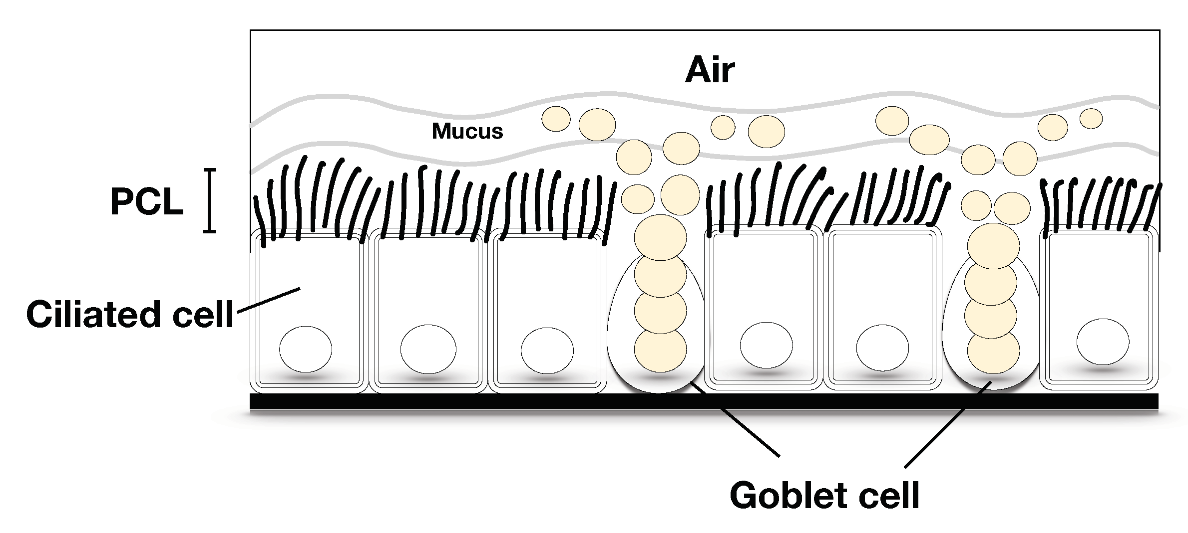
Figure 2.
The free surface and the porous region on the axis when (a) the cilia are perpendicular to the horizontal plane; (b) the cilia make a angle with the horizontal plane.
Figure 2.
The free surface and the porous region on the axis when (a) the cilia are perpendicular to the horizontal plane; (b) the cilia make a angle with the horizontal plane.
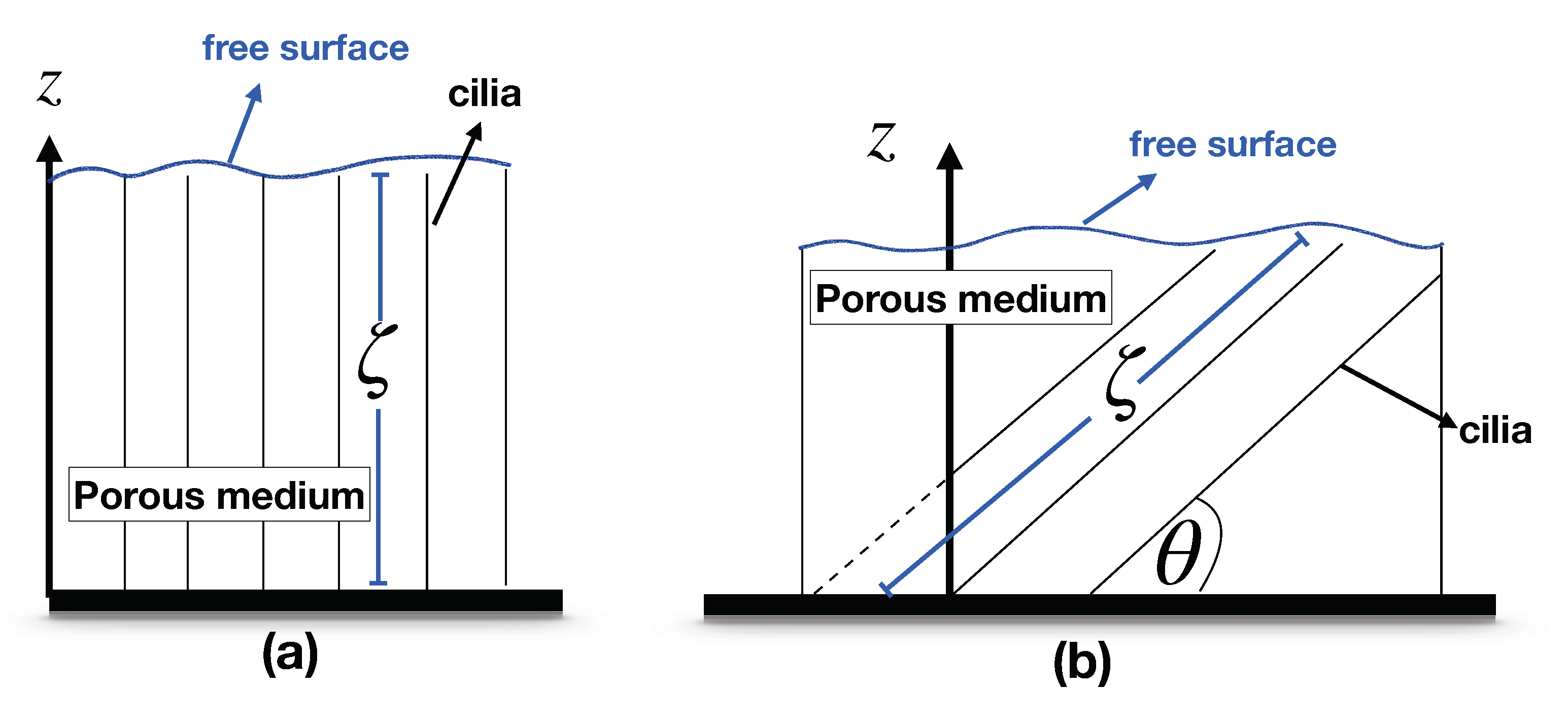
Figure 3.
Fluid flow over the porous medium.

Figure 4.
Physical (above) and natural (below) coordinates.
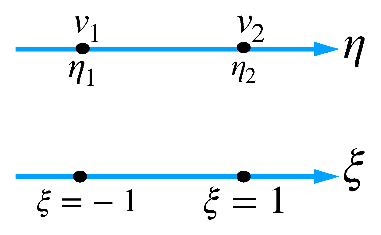
Figure 5.
Velocities of the periciliary layer (PCL) fluid and the exact solution when the angle is perpendicular to the horizontal plane.
Figure 5.
Velocities of the periciliary layer (PCL) fluid and the exact solution when the angle is perpendicular to the horizontal plane.
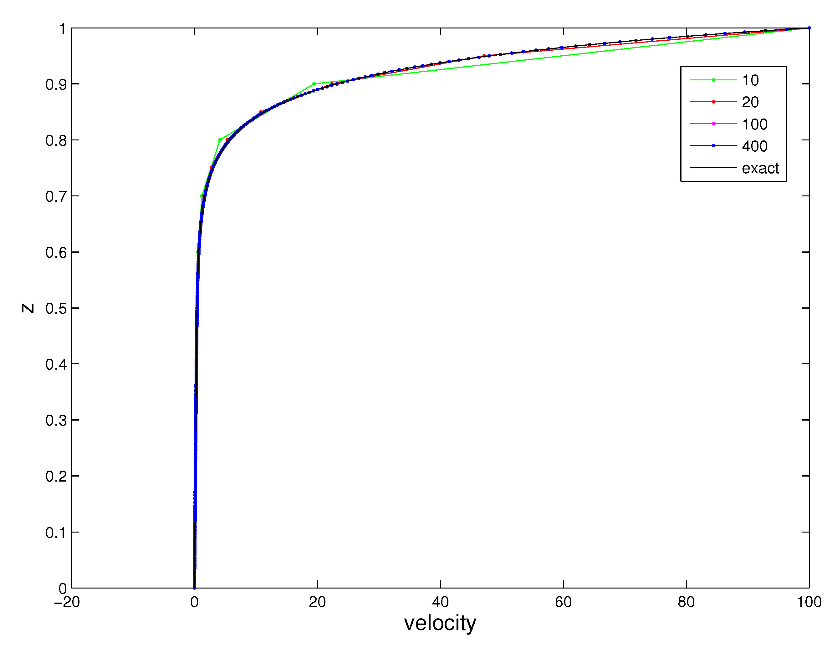
Figure 6.
The velocities of the PCL fluid for the angles to .
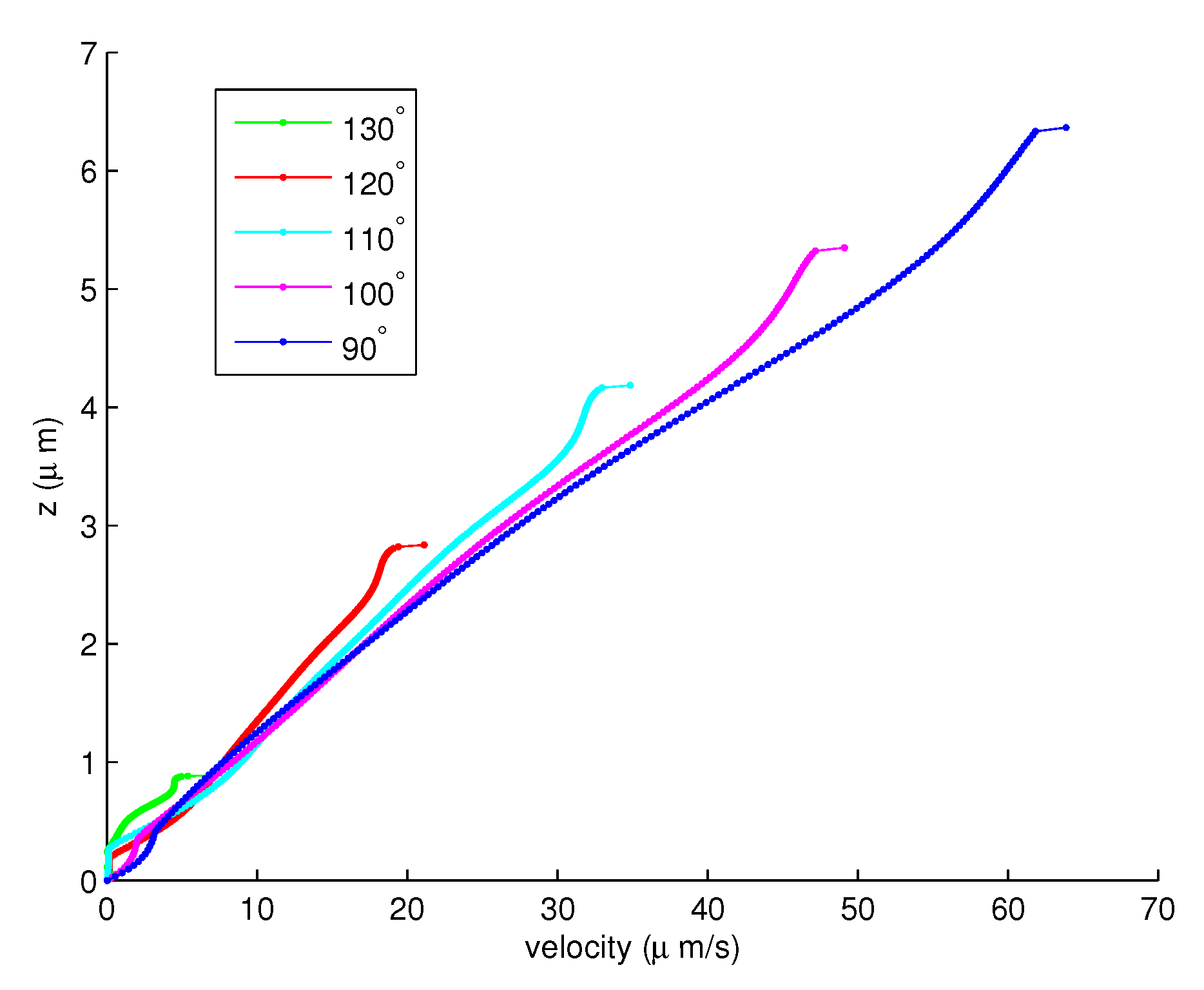
Figure 7.
The velocities of the PCL fluid for the angles to .
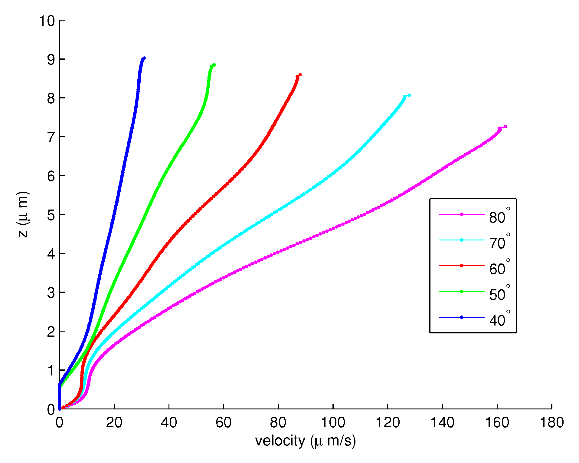
Figure 8.
The velocities of PCL fluid for the full forward stroke of the cilia from the angles to .
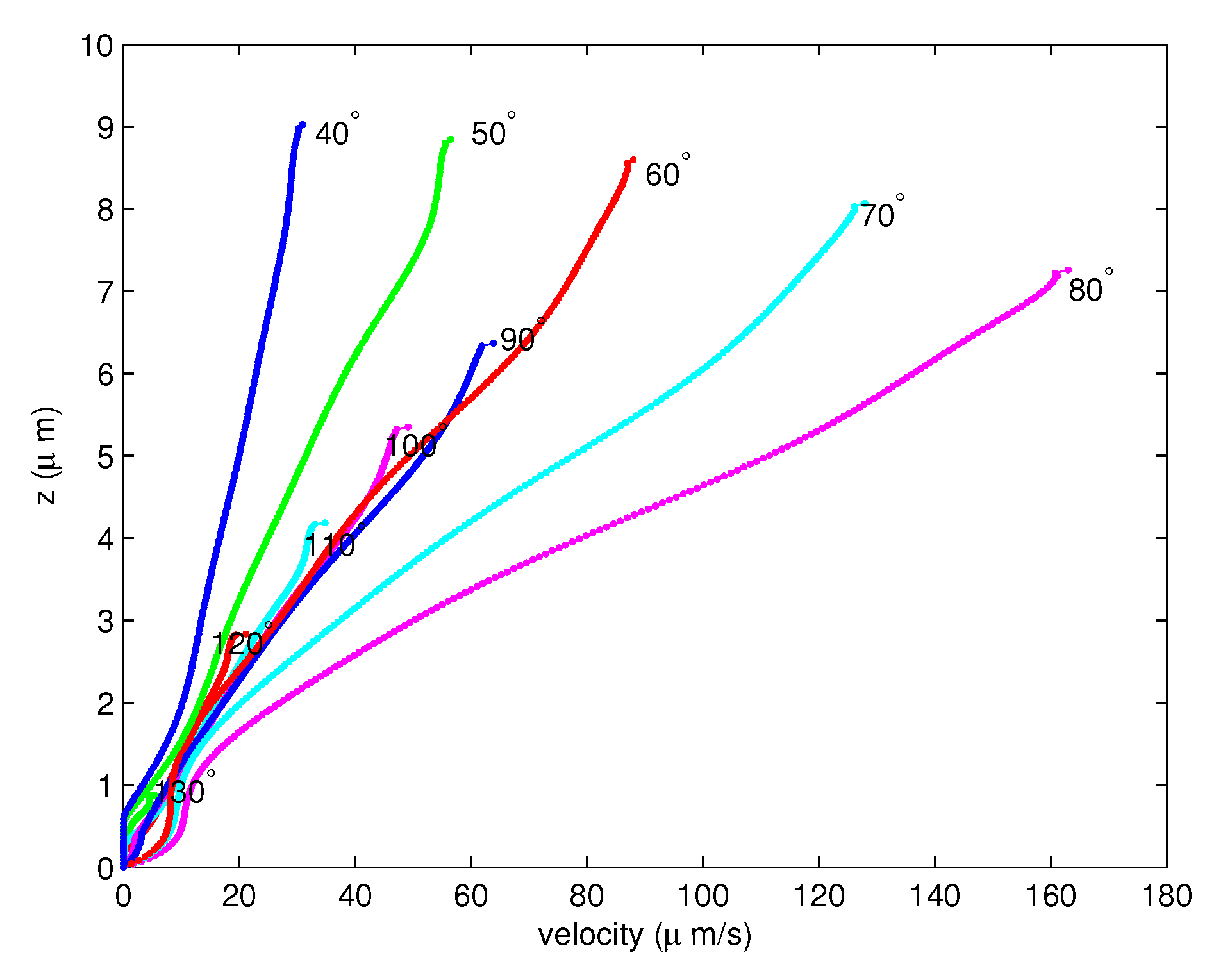
Figure 9.
The average velocities for each angle .
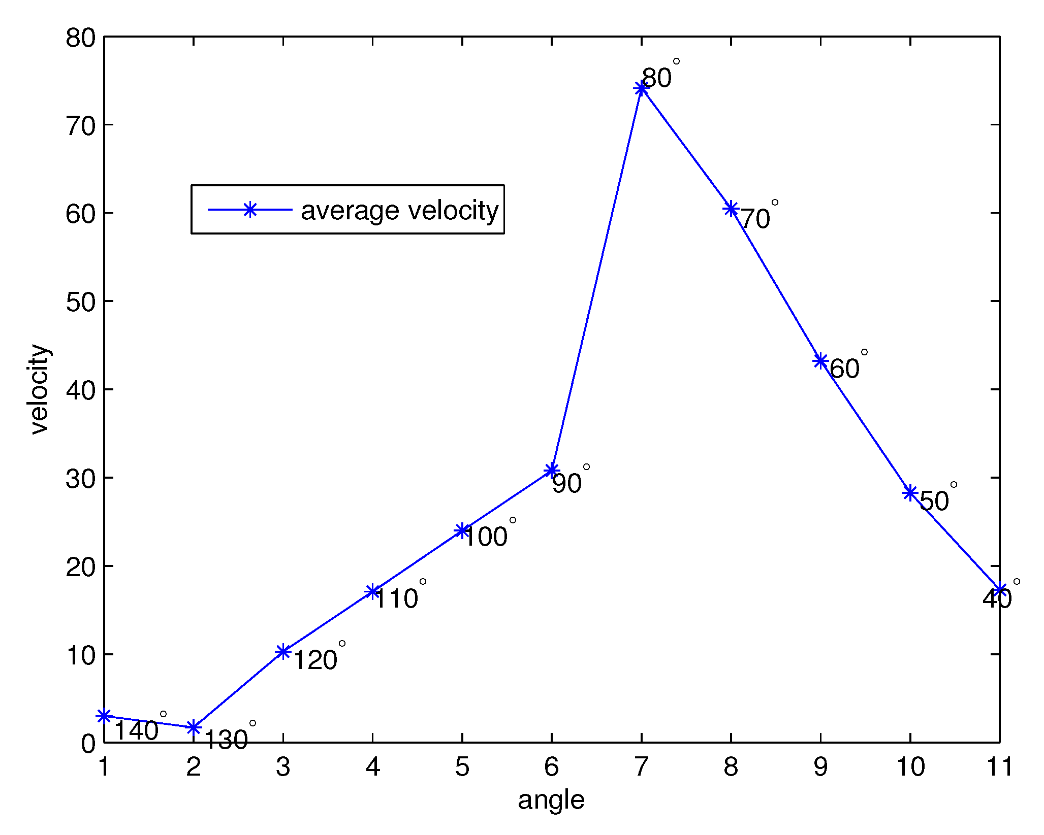
Figure 10.
The free surface for the forward stroke at the tips of the cilia.
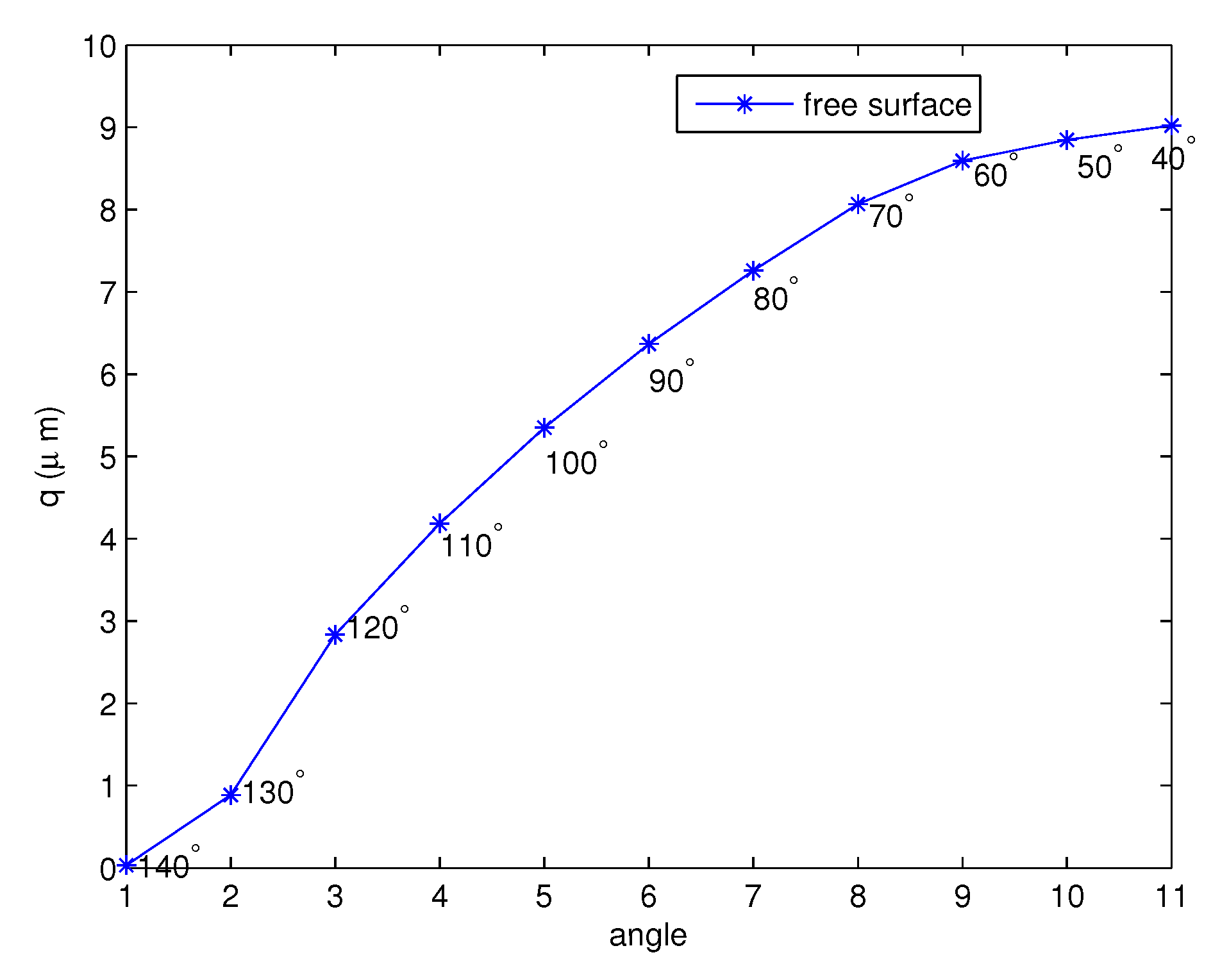
Figure 11.
The free surface for the forward stroke at the tips of the cilia at different values of c when .
Figure 11.
The free surface for the forward stroke at the tips of the cilia at different values of c when .
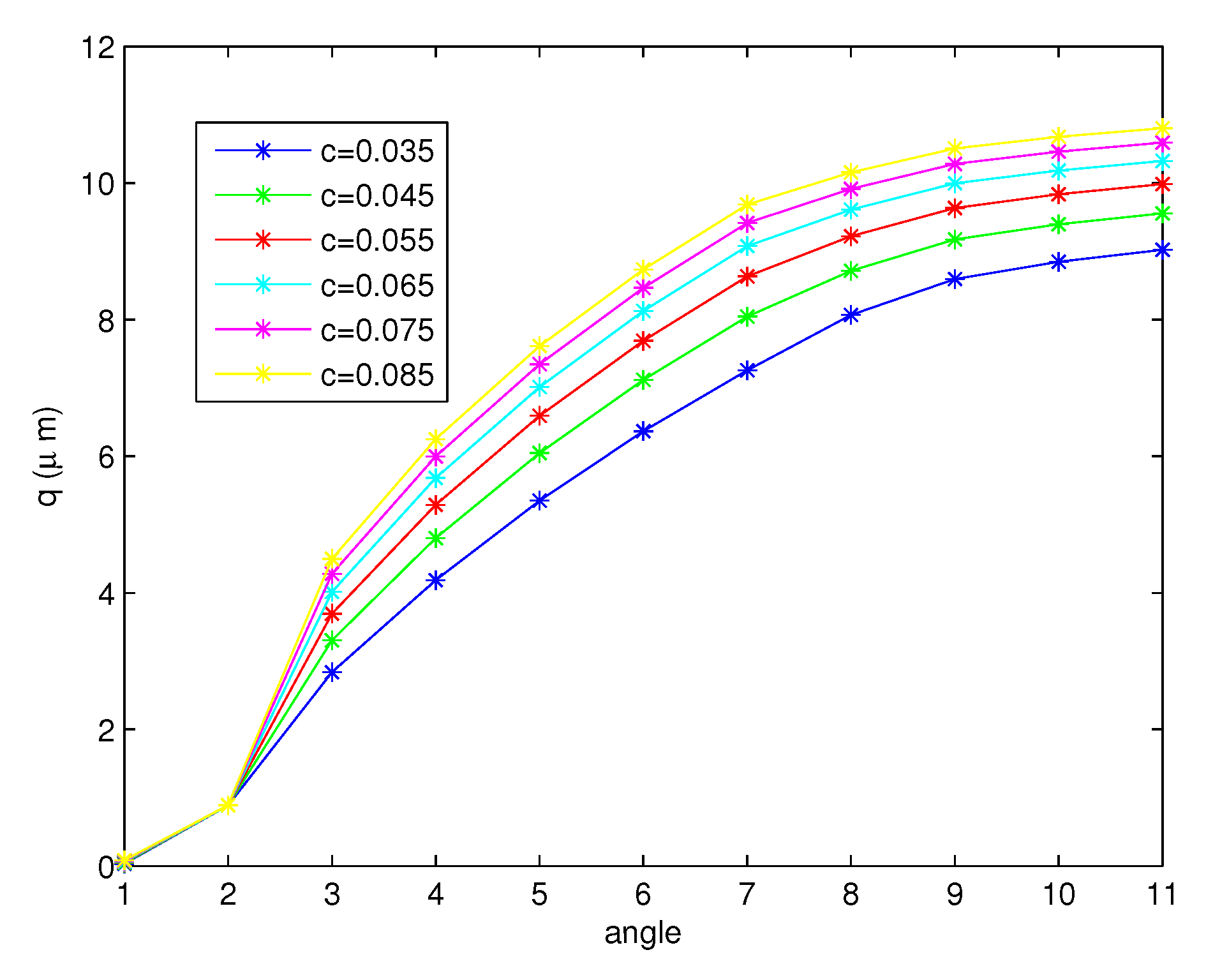
Figure 12.
The free surface for the forward stroke at the tips of the cilia at different values of c when .
Figure 12.
The free surface for the forward stroke at the tips of the cilia at different values of c when .

Table 1.
-norm errors of the PCL velocity at the angle along the z-axis with fixed boundary conditions.
Table 1.
-norm errors of the PCL velocity at the angle along the z-axis with fixed boundary conditions.
| Number of Nodes along z-Axis | -Norm Errors |
|---|---|
| 10 | 4.0837 |
| 20 | 1.3711 |
| 100 | 0.1184 |
| 400 | 0.0148 |
Publisher’s Note: MDPI stays neutral with regard to jurisdictional claims in published maps and institutional affiliations. |
© 2020 by the author. Licensee MDPI, Basel, Switzerland. This article is an open access article distributed under the terms and conditions of the Creative Commons Attribution (CC BY) license (http://creativecommons.org/licenses/by/4.0/).
Share and Cite
MDPI and ACS Style
Wuttanachamsri, K. Free Interfaces at the Tips of the Cilia in the One-Dimensional Periciliary Layer. Mathematics 2020, 8, 1961. https://doi.org/10.3390/math8111961
AMA Style
Wuttanachamsri K. Free Interfaces at the Tips of the Cilia in the One-Dimensional Periciliary Layer. Mathematics. 2020; 8(11):1961. https://doi.org/10.3390/math8111961
Chicago/Turabian StyleWuttanachamsri, Kanognudge. 2020. "Free Interfaces at the Tips of the Cilia in the One-Dimensional Periciliary Layer" Mathematics 8, no. 11: 1961. https://doi.org/10.3390/math8111961
Note that from the first issue of 2016, this journal uses article numbers instead of page numbers. See further details here.