A New Family of Extended Lindley Models: Properties, Estimation and Applications

Abstract

There are many proposed life models in the literature, based on Lindley distribution. In this paper, a unified approach is used to derive a general form for these life models. The present generalization greatly simplifies the derivation of new life distributions and significantly increases the number of lifetime models available for testing and fitting life data sets for biological, engineering, and other fields of life. Several distributions based on the disparity of the underlying weights of Lindley are shown to be special cases of these forms. Some basic statistical properties and reliability functions are derived for the general forms. In addition, comparisons among various forms are investigated. Moreover, the power distribution of this generalization has also been considered. Maximum likelihood estimator for complete and right-censored data has been discussed and in simulation studies, the efficiency and behavior of it have been investigated. Finally, the proposed models have been fit to some data sets.

1. Introduction

In recent years, one notes an increasing need for varieties of lifetime distributions to make the wealth of life models available for nicely fitting life lengths. These models are utilized for many products, systems, and reliability operations such as replacement and maintenance. In addition, reliability analysis requires the study of failure rates, mean residual life, and other aging properties of the product, which heavily depend on the form of the underlying model. Furthermore, the generalization would significantly increase the life models available for testing and fitting real-life data sets for biological, engineering, actuarial, medical, and other fields of life. It is known that appropriate modeling of data may provide a deeper insight of data, which shows its characteristics and makes its asymptotic behavior traceable (cf. Tobias [1], Wolstenholme [2], Schwartz [3] and McPherson [4]). In this context, many authors have proposed some generalizations of Lindley [5], whose probability density function (pdf) is given by

$$f\left(x\right)=\frac{{\theta }^2}{1+\theta }(1+x)e^{-\theta x},\theta >0,x\ge 0.$$

(1)

It is a mixture of two gamma distributions $G(1,\theta )$ and $G(2,\theta )$, respectively, with weights $\frac{\theta }{1+\theta }$ and $\frac{1}{1+\theta }$. The cumulative distribution function (CDF) of Lindley is

$$F\left(x\right)=1-\frac{1+\theta +\theta x}{1+\theta }{e}^{-\theta x},\theta >0,x\ge 0.$$

(2)

The Lindley model was used to analyze failure rate data and stress-strength reliability models. This distribution and its other generalizations lie on the recent developments of new flexible families and provide great flexibility in modeling lifetime data, see for example Ghitany et al. [6,7], Bakouch et al. [8], Abouammoh et al. [9] and Cakmakyapan and Ozel [10].

One important drawback of the Lindley model is that it is not scale invariant. One distribution family $f\left(x\right)$ is said to be scale invariant if by changing x to $kx$, $k>0$, the family does not change. So, changing the scale or units of x leaves the fit invariant. Shanker and Mishra [11] introduced one quasi Lindley model that is scale invariant.

In this paper, we consider scale invariant generalizations of the Lindley distribution that utilize some changes of the mixing weights, which give more flexibility to the mixed distributions. The plan of this paper is as follows. Section 2 gives a generalization of the Lindley model based on the change of the weight parameters and some of its main statistical and reliability properties are investigated. In addition, in that section, the special cases that yield some earlier proposed models in the literature are explored. Then, another extension has been introduced and its main properties are discussed. In Section 3, estimating the parameter(s) of the proposed model has been studied. In Section 4, the results of a simulation study have been briefly presented. In Section 5, the proposed models have been utilized to fit some real lifetime data sets. Finally, in Section 6, we give a brief conclusion and some remarks on the current and future of this research.

2. Generalization Based on Mixing Weights

In the literature, one direct generalization of the Lindley distribution is to consider different values for mixing weights. In this context, we propose a relatively similar, but new and comprehensive approach to introduce a series of general distributions.

Definition 1.

The non-negative random variable X is said to follow the Abouammoh–Kayid model with parameters α, β, δ and θ, abbreviated by $AK(\alpha ,\beta ,\delta ,\theta )$, when its PDF is given by

$$f\left(x\right)=\frac{\theta }{{\Gamma }\left(\alpha \right)+{\delta }^{\alpha +\beta -1}}({\delta }^{\alpha +\beta -1}+{\left(\theta x\right)}^{\alpha -1})e^{-\theta x},x\ge 0,\alpha >0,\beta >0,\delta >0,\theta >0,$$

(3)

which is a mixture of the gamma distributions $G(1,\theta )$ and $G(\alpha ,\theta )$ with weights $p=\frac{{\delta }^{\alpha +\beta -1}}{{\Gamma }\left(\alpha \right)+{\delta }^{\alpha +\beta -1}}$ and $1-p$, respectively.

The CDF of this model is

$$F\left(x\right)=1-\frac{{\delta }^{\alpha +\beta }{e}^{-\theta x}+\delta {\Gamma }(\theta x,\alpha )}{\delta {\Gamma }\left(\alpha \right)+{\delta }^{\alpha +\beta }},$$

(4)

where ${\Gamma }(t,n)={\int }_t^{\infty }{y}^{n-1}{e}^{-y}dy$ shows the upper incomplete function. When $\delta =\theta$, $\alpha =2$ and $\beta =0$, $AK(\alpha ,\beta ,\delta ,\theta )$ reduces to the well-known Lindley model.

Proposition 1.

If $X\sim AK(\alpha ,\beta ,\delta ,\theta )$, then its k^th moment is given by

$$E\left(X^k\right)=\frac{1}{{\theta }^k}\frac{{\delta }^{\alpha +\beta }{\Gamma }(k+1)+\delta {\Gamma }(k+\alpha )}{{\delta }^{\alpha +\beta }+\delta {\Gamma }\left(\alpha \right)}.$$

(5)

Proof. 

We have

$$\begin{array}{cc}\hfill E\left(X^k\right)& ={\int }_0^{\infty }{x}^k\frac{\theta }{{\Gamma }\left(\alpha \right)+{\delta }^{\alpha +\beta -1}}({\delta }^{\alpha +\beta -1}+{\left(\theta x\right)}^{\alpha -1})e^{-\theta x}dx\hfill \\ \hfill & =\frac{\theta {\delta }^{\alpha +\beta -1}}{{\Gamma }\left(\alpha \right)+{\delta }^{\alpha +\beta -1}}{\int }_0^{\infty }{x}^k{e}^{-\theta x}dx+\frac{{\theta }^{\alpha }}{{\Gamma }\left(\alpha \right)+{\delta }^{\alpha +\beta -1}}{\int }_0^{\infty }{x}^{k+\alpha -1}{e}^{-\theta x}dx\hfill \\ \hfill & =\frac{\theta {\delta }^{\alpha +\beta -1}}{{\Gamma }\left(\alpha \right)+{\delta }^{\alpha +\beta -1}}\frac{{\Gamma }(k+1)}{{\theta }^{k+1}}+\frac{{\theta }^{\alpha }}{{\Gamma }\left(\alpha \right)+{\delta }^{\alpha +\beta -1}}\frac{{\Gamma }(k+\alpha )}{{\theta }^{k+\alpha }}\hfill \\ \hfill & =\frac{1}{{\theta }^k}\frac{{\delta }^{\alpha +\beta }{\Gamma }(k+1)+\delta {\Gamma }(k+\alpha )}{{\delta }^{\alpha +\beta }+\delta {\Gamma }\left(\alpha \right)},\hfill \end{array}$$

which shows the result. □

By setting $k=1$ and 2 in Proposition 1, the mean and variance of the distribution can be computed directly. The moment generating function of $AK(\alpha ,\beta ,\delta ,\theta )$ has the following closed form:

$$E\left(e^{tX}\right)=\frac{1}{{\Gamma }\left(\alpha \right)+{\delta }^{\alpha +\beta -1}}\left({\delta }^{\alpha +\beta -1}\frac{\theta }{\theta -t}+{\Gamma }\left(\alpha \right)\frac{{\theta }^{\alpha }}{{(\theta -t)}^{\alpha }}\right).$$

(6)

The failure rate function can be simplified to

$$h\left(x\right)=\frac{{\delta }^{\alpha +\beta -1}+{\left(\theta x\right)}^{\alpha -1}}{{\delta }^{\alpha +\beta -1}+e^{\theta x}{\Gamma }(\theta x,\alpha )}\theta .$$

(7)

Figure 1 and Figure 2 present the graphs of density and failure rate functions for the $AK(\alpha ,\beta ,\delta ,\theta )$ random variables for some values of parameters. The shape of the failure rate function is useful in describing the lifetime model, for example, when we have an instrument/creature that deteriorates with time we expect that its corresponding failure rate function will be increasing. Similarly, a bathtub shaped failure rate function may be useful for modeling the lifetime of an object that is very fragile at the beginning of its life, one may refer to Lai and Xie [12] for more details. Figure 2 reveals that the failure rate function accommodates increasing, decreasing and bathtub shape. It seems that for larger values of $\alpha$, the density function has a thicker tail.

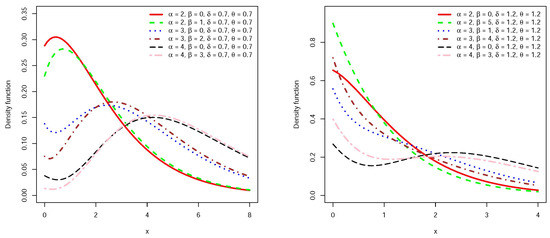
Figure 1. Density function for $AK(\alpha ,\beta ,\delta ,\theta )$ for some $\alpha$, $\beta$, $\delta$ and $\theta$ values.

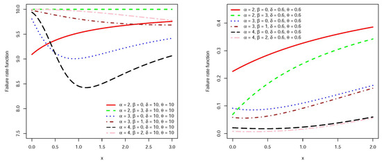
Figure 2. Failure rate function of $AK(\alpha ,\beta ,\delta ,\theta )$ for some parameter values.

The concept of mean residual life (MRL) plays an important role in reliability and life testing. The next proposition provides the MRL of $AK(\alpha ,\beta ,\delta ,\theta )$.

Proposition 2.

If $X\sim AK(\alpha ,\beta ,\delta ,\theta )$, then its MRL is given by

$$m\left(x\right)=\frac{1}{{\delta }^{\alpha +\beta -1}{e}^{-\theta x}+{\Gamma }(\theta x,\alpha )}(\frac{1}{\theta }({\delta }^{\alpha +\beta -1}+{\left(\theta x\right)}^{\alpha })e^{-\theta x}+(\frac{\alpha }{\theta }-x){\Gamma }(\theta x,\alpha )).$$

(8)

Proof. 

First, the MRL is given by

$$m\left(x\right)=\frac{1}{R\left(x\right)}{\int }_x^{\infty }R\left(t\right)dt,$$

(9)

where $R\left(x\right)=1-F\left(x\right)$ is the reliability function. However, we have

$${\int }_x^{\infty }R\left(t\right)dt=\frac{1}{{\delta }^{\alpha +\beta -1}+{\Gamma }\left(\alpha \right)}({\int }_x^{\infty }{\delta }^{\alpha +\beta -1}{e}^{-\theta t}dt+{\int }_x^{\infty }{\Gamma }(\theta t,\alpha )dt).$$

(10)

It is straightforward to show that the first integral inside parentheses reduces to $\frac{1}{\theta }{\delta }^{\alpha +\beta -1}{e}^{-\theta x}$. However, the second integral can be simplified by some algebra as follows:

$$\begin{array}{cc}\hfill {\int }_x^{\infty }{\Gamma }(\theta t,\alpha )dt& ={\int }_x^{\infty }{\int }_{\theta t}^{\infty }{y}^{\alpha -1}{e}^{-y}dydt\hfill \\ \hfill & ={\int }_{\theta x}^{\infty }{\int }_x^{\frac{y}{\theta }}{y}^{\alpha -1}{e}^{-y}dtdy\hfill \\ \hfill & ={\int }_{\theta x}^{\infty }(\frac{y}{\theta }-x)y^{\alpha -1}{e}^{-y}dy\hfill \\ \hfill & =\frac{1}{\theta }{\Gamma }(\theta x,\alpha +1)-x{\Gamma }(\theta x,\alpha )\hfill \\ \hfill & =\frac{1}{\theta }{\left(\theta x\right)}^{\alpha }{e}^{-\theta x}+(\frac{\alpha }{\theta }-x){\Gamma }(\theta x,\alpha ).\hfill \end{array}$$

(11)

The last equation in (11), follows from the fact that ${\Gamma }(x,\alpha +1)=\alpha {\Gamma }(x,\alpha )+x^{\alpha }{e}^{-x}$. Appealing to (10) and (11), the required result follows. □

2.1. Some Special Cases of $AK(\alpha ,\beta ,\delta ,\theta )$

In this subsection, we derive some special cases of the $AK(\alpha ,\beta ,\delta ,\theta )$ for various values of the parameters that have been introduced in the literature. In the special case $\delta =\theta$, the following more special cases have been studied in the literature.

Case 1.

For $\alpha =2$ and $\beta =0$, $AK(\alpha ,\beta ,\delta ,\theta )$ reduces to the well-known Lindley model.

Case 2.

When $\alpha =3$ and $\beta =0$, it reduces to the Akash distribution proposed and studied by Shanker [13].

Case 3.

For $\alpha =6$ and $\beta =0$, we have the Prakaamy distribution, which was introduced and discussed by Shukla [14].

Case 4.

For $\alpha =2$ and $\beta =1$, it reduces to the Shanker distribution, which was proposed and studied by Shanker [15].

Case 5.

For $\alpha =3$ and $\beta =1$, it is the Isheta distribution introduced and studied by Shanker and Shukla [16].

Case 6.

For $\alpha =4$ and $\beta =1$, it reduces to the Pranav distribution proposed by Shukla [17].

Case 7.

For $\alpha =6$ and $\beta =1$, we have the Ram Awadh distribution, which was introduced and discussed by Shukla [18].

One can verify that all statistical and reliability properties of these special cases can be obtained from the corresponding property of $AK(\alpha ,\beta ,\delta ,\theta )$ by utilizing appropriate values for $\alpha$ and $\beta$.

2.2. Power Generalization

Many generalizations of the well-known Lindley [5] distribution are special cases of $AK(\alpha ,\beta ,\delta ,\theta )$ family. Here we propose a new model that extends $AK(\alpha ,\beta ,\delta ,\theta )$.

Definition 2.

A non-negative random variable X is said to have the power $AK(\alpha ,\beta ,\delta ,\theta )$ distribution, denoted by $PAK(\alpha ,\beta ,\delta ,\theta ,\gamma )$, if its PDF is given by

$$f\left(x\right)=\frac{\theta \gamma x^{\gamma -1}}{{\Gamma }\left(\alpha \right)+{\delta }^{\alpha +\beta -1}}({\delta }^{\alpha +\beta -1}+{\left(\theta x^{\gamma }\right)}^{\alpha -1})e^{-\theta x^{\gamma }},x\ge 0,\alpha >0,\beta >0,\delta >0,\theta >0,\gamma >0,$$

(12)

Note that if $X\sim AK(\alpha ,\beta ,\delta ,\theta )$ then $X^{\frac{1}{\gamma }}\sim PAK(\alpha ,\beta ,\delta ,\theta ,\gamma )$. This statement is useful for studying the statistical and reliability properties of this extended model. The corresponding CDF of the above density is

$$F\left(x\right)=1-\frac{{\delta }^{\alpha +\beta }{e}^{-\theta x^{\gamma }}+\delta {\Gamma }(\theta x^{\gamma },\alpha )}{\delta {\Gamma }\left(\alpha \right)+{\delta }^{\alpha +\beta }}.$$

(13)

For $\alpha =1$ and $\delta =1$, $PAK(\alpha ,\beta ,\delta ,\theta ,\gamma )$ reduces to the well-known Weibull model with CDF

$$F\left(x\right)=1-e^{-\theta x^{\gamma }}.$$

Proposition 3.

Let $X\sim PAK(\alpha ,\beta ,\delta ,\theta ,\gamma )$, then, its k^th moment is

$$E\left(X^k\right)={\theta }^{-\frac{k}{\gamma }}\frac{{\delta }^{\alpha +\beta }{\Gamma }(\frac{k}{\gamma }+1)+\delta {\Gamma }(\frac{k}{\gamma }+\alpha )}{{\delta }^{\alpha +\beta }+\delta {\Gamma }\left(\alpha \right)}.$$

(14)

Proof. 

Let $T\sim AK(\alpha ,\beta ,\delta ,\theta )$, then $X=T^{\frac{1}{\gamma }}\sim PAK(\alpha ,\beta ,\delta ,\theta ,\gamma )$. Thus, $E(X^k)=E(T^{\frac{k}{\alpha }})$. So, the result follows by (5) directly. □

The failure rate function of $PAK(\alpha ,\beta ,\delta ,\theta ,\gamma )$ is

$$h\left(x\right)=\gamma x^{\gamma -1}\frac{{\delta }^{\alpha +\beta -1}+{\left(\theta x^{\gamma }\right)}^{\alpha -1}}{{\delta }^{\alpha +\beta -1}+e^{\theta x^{\gamma }}{\Gamma }(\theta x^{\gamma },\alpha )}\theta .$$

(15)

3. Estimation of Parameters for the Complete and Right Censored Data

The proposed distributions (3) and (12) have four and five parameters, respectively, which makes the estimation process very complicated. To overcome the complexity, we assume two parameters $\alpha$ and $\beta$ in a discrete subspace. In this way, we take $\alpha =1,2,3,\dots$ and $\beta =0,1,2,\dots$. We take a proper set of pairs $(\alpha ,\beta )$ and, for each pair, estimate the remaining parameters by moments or maximum likelihood methods. Then, we can choose the best $(\alpha ,\beta )$ based on the Kolmogorov–Smirnov (K-S) or similar statistics.

Let $X_i$, $i=1,2,\cdots ,v$ be an independent and identically distributed (iid) random sample of $AK(\alpha ,\beta ,\delta ,\theta )$. For known ($\alpha$, $\beta$), by (5), one estimator for ($\theta$, $\delta$) can be derived by solving the following system of equations in terms of $(\delta ,\theta )$.

$$\left\{\begin{array}{c}\overline{X}=\frac{1}{\theta }\frac{{\delta }^{\alpha +\beta }+\delta {\Gamma }(\alpha +1)}{{\delta }^{\alpha +\beta }+\delta {\Gamma }\left(\alpha \right)},\hfill \\ \overline{X^2}=\frac{1}{{\theta }^2}\frac{2{\delta }^{\alpha +\beta }+\delta {\Gamma }(\alpha +2)}{{\delta }^{\alpha +\beta }+\delta {\Gamma }\left(\alpha \right)}.\hfill \end{array}\right.$$

(16)

The second fraction in Equation (16), is greater than one, so one lower bound for the estimate of $\theta$ is $max(\frac{1}{\overline{X}},{(\frac{1}{\overline{X^2}})}^{0.5})$. This bound can be very helpful in finding a solution of (16) or optimizing likelihood function and computing maximum likelihood estimation. It can be applied as a good initial point in maximizing the log-likelihood function.

Assume that $x_i$, $i=1,2,\cdots ,v$ represents a realization of the mentioned random sample of $AK(\alpha ,\beta ,\delta ,\theta )$. The log-likelihood function of $(\delta ,\theta )$, with known $(\alpha ,\beta )$, is

$$l(\delta ,\theta ;\mathbf{x})=vln\theta -vln({\Gamma }\left(\alpha \right)+{\delta }^{\alpha +\beta -1})+\sum _{i=1}^{v}ln({\delta }^{\alpha +\beta -1}+{\left(\theta x_i\right)}^{\alpha -1})-\theta \sum _{i=1}^v{x}_i.$$

(17)

The score statistics can be obtained by differentiating of log-likelihood function in terms of $\delta$ and $\theta$.

$$\frac{\partial l(\delta ,\theta ;\mathbf{x})}{\partial \delta }=-v\frac{(\alpha +\beta -1){\delta }^{\alpha +\beta -2}}{{\Gamma }\left(\alpha \right)+{\delta }^{\alpha +\beta -1}}+\sum _{i=1}^v\frac{(\alpha +\beta -1){\delta }^{\alpha +\beta -2}}{{\delta }^{\alpha +\beta -1}+{\left(\theta x_i\right)}^{\alpha -1}},$$

(18)

and

$$\frac{\partial l(\delta ,\theta ;\mathbf{x})}{\partial \theta }=\frac{v}{\theta }+\sum _{i=1}^v\frac{(\alpha -1)x_i{\left(\theta x_i\right)}^{\alpha -2}}{{\delta }^{\alpha +\beta -1}+{\left(\theta x_i\right)}^{\alpha -1}}-\sum _{i=1}^v{x}_i.$$

(19)

The maximum likelihood estimator (MLE) can be computed by maximizing (17) in terms of $\theta$, or by solving the equation $\frac{\partial l(\delta ,\theta ;\mathbf{x})}{\partial \delta }=0$ and $\frac{\partial l(\delta ,\theta ;\mathbf{x})}{\partial \theta }=0$ for ($\delta$,$\theta$). We apply the first approach in the next section to investigate the practical potential of MLE and study the behavior of this estimator by a simulation study. The log-likelihood function when $x_i$, $i=1,2,\cdots ,v$ represents a realization of $PAK(\alpha ,\beta ,\delta ,\theta ,\gamma )$, with known $\alpha$ and $\beta$, is

$$\begin{array}{cc}\hfill l(\delta ,\theta ,\gamma ;\mathbf{x})& =vln\gamma +(\gamma -1)\sum _{i=1}^{v}ln{x}_i+vln\theta -vln({\Gamma }\left(\alpha \right)+{\delta }^{\alpha +\beta -1})\hfill \\ \hfill & +\sum _{i=1}^{v}ln({\delta }^{\alpha +\beta -1}+{\left(\theta x_i^{\gamma }\right)}^{\alpha -1})-\theta \sum _{i=1}^v{x}_i^{\gamma }.\hfill \end{array}$$

(20)

Let $X_i$ represent a random lifetime, which is censored by a random variable $C_i$ such that $X_i$ is observed when $X_i\le C_i$ and otherwise all information about $X_i$ is that it is greater than $C_i$. In this case $X_i$ is said to be right censored by $C_i$. In other words, the observations consist of $T_i=min\{X_i,C_i\}$ and $D_i$, which equals 1 when $X_i\le C_i$ and 0 when $X_i>C_i$ (cf. Fleming and Harrington [19]). The log-likelihood of $AK(\alpha ,\beta ,\delta ,\theta )$ ($PAK(\alpha ,\beta ,\delta ,\theta ,\gamma )$) for censored data $t_i$ and $d_i$, $i=1,2,\cdots ,v$ is denoted by $l(\delta ,\theta ;\mathbf{t},\mathbf{d})\left(l\right(\delta ,\theta ,\gamma ;\mathbf{t},\mathbf{d}\left)\right)$ and equal to

$$\sum _{i=1}^v{d}_{i}lnf\left(t_i\right)+\sum _{i=1}^v(1-d_i)lnR\left(t_i\right),$$

(21)

where $f_i$ and $R_i$ show pdf and reliability function of $AK(\alpha ,\beta ,\delta ,\theta )$ ($PAK(\alpha ,\beta ,\delta ,\theta ,\gamma )$), respectively.

4. Simulation Study

Generating random samples of $AK(\alpha ,\beta ,\delta ,\theta )$ can be obtained from the fact that the model is a mixture of two gamma distributions. In this way, we have the following steps:

• Generate one sample of multinomial distribution with parameters v, $p=\frac{{\delta }^{\alpha +\beta -1}}{{\Gamma }\left(\alpha \right)+{\delta }^{\alpha +\beta -1}}$ and $1-p$. Suppose that the generated instance be denoted by $k_1$ and $k_2$, corresponding respectively to probabilities p and $1-p$. Note that $k_1+k_2=v$.
• Simulate one sample from gamma model $G(1,\theta )$ with size $k_1$ and another sample from $G(\alpha ,\theta )$ with size $k_2$. We merge these two samples to have one sample of $AK(\alpha ,\beta ,\delta ,\theta )$ with size v.

In cases where we need right censored samples, the uniform r.v. on an interval $[0,t_{*}]$ has been considered as $C_i$. Given p, the censorship percentage, we find $t_{*}$ by solving the following equation in terms of $t_{*}$.

$${\int }_0^{t_{*}}R\left(u\right)du=p{t}_{*},$$

(22)

which can be solved numerically.

Table 1 presents the results of our simulation study for $AK(\alpha ,\beta ,\delta ,\theta )$ distribution. Two censorship levels $p=0$ (uncensored) and $p=0.20$ (20 percent of instances have been censored) have been considered. In every run, we derive $w=500$ replicates of samples of size v. Then for every replicate, the MLE for $(\delta ,\theta )$, $(\widehat{\delta },\widehat{\theta })$, has been computed by maximizing the log-likelihood function (21). In this order, from top to bottom, every cell consists of three measurements $(B_{\delta },B_{\theta })$, $(A{B}_{\delta },A{B}_{\theta })$ and $(MS{E}_{\delta },MS{E}_{\theta })$ where

$$B_{\delta }=\frac{1}{w}\sum _{i=1}^w({\widehat{\delta }}_i-\delta ),$$

(23)

$$A{B}_{\delta }=\frac{1}{w}\sum _{i=1}^w|{\widehat{\delta }}_i-\delta |,$$

(24)

and

$$MS{E}_{\delta }=\frac{1}{w}\sum _{i=1}^w{({\widehat{\delta }}_i-\delta )}^2,$$

(25)

and $B_{\theta }$, $A{B}_{\theta }$ and $MS{E}_{\theta }$ are defined similarly. From Table 1, some observations abstracted are listed here.

Table 1. Simulation results for $AK(\alpha ,\beta ,\delta ,\theta )$. Every cell consists of pairs $(B_{\delta },B_{\theta })$, $(A{B}_{\delta },A{B}_{\theta })$ and $(MS{E}_{\delta },MS{E}_{\theta })$ from top to bottom.

		$\mathit{p}=0$		$\mathit{p}=0.20$
$\mathit{v}$	$(\mathbf{\alpha },\mathbf{\beta })$	$\mathbf{\delta }=\mathbf{0.2},\mathbf{\theta }=\mathbf{1.2}$	$\mathbf{\delta }=\mathbf{0.4},\mathbf{\theta }=\mathbf{0.05}$	$\mathbf{\delta }=\mathbf{0.2},\mathbf{\theta }=\mathbf{1.2}$	$\mathbf{\delta }=\mathbf{0.4},\mathbf{\theta }=\mathbf{0.05}$
30	(2,1)	(0.013000, −0.007520)	(0.013888, 0.001214)	(0.313307, −0.021339)	(0.458239, −0.000243)
		(0.237531, 0.145039)	(0.376828, 0.006787)	(0.541801, 0.164034)	(0.821119, 0.007860)
		(0.092244, 0.034001)	(1.440460, 0.000074)	(7.131440, 0.057312)	(7.109937, 0.000109)
	(3,2)	(−0.044634, -.004039)	(−0.190346, 0.000018)	(−0.045337, −0.007946)	(−0.163909, −0.000265)
		(0.239059, 0.105796)	(0.326939, 0.004271)	(0.234000, 0.111629)	(0.355852, 0.005062)
		(0.089102, 0.018373)	(0.116500, 0.000029)	(0.066341, 0.019126)	(0.631660, 0.000043)
50	(2,1)	(−0.010284, 0.005392)	(−0.045135, 0.000987)	(0.030007, −0.004096)	(0.07146, −0.000103)
		(0.195604, 0.109608)	(0.244568, 0.005464)	(0.248331, 0.119299)	(0.363505, 0.005866)
		(0.055114, 0.019733)	(0.109090, 0.000048)	(0.977620, 0.023694)	(2.245982, 0.000057)
	(3,2)	(−0.049990, −0.002405)	(−0.187037, 0.000247)	(−0.054677, −0.006306)	(−0.176889, −0.000140)
		(0.222270, 0.078619)	(0.301444, 0.003425)	(0.221826, 0.088594)	(0.301239, 0.003759)
		(0.056555, 0.009928)	(0.103816, 0.000018)	(0.058013, 0.012358)	(0.103287, 0.000022)

• Absolute means of biases ($A{B}_{\delta },A{B}_{\theta }$), have greater values for censored samples.
• ($A{B}_{\delta },A{B}_{\theta }$) and ($MS{E}_{\delta },MS{E}_{\theta }$) show smaller for larger sample size, v.
• $B_{\delta }$, $A{B}_{\delta }$ and $MS{E}_{\delta }$ increase with $\delta$ and a similar statement holds for $\theta$.

Table 2 gathers results of our simulation study for $PAK(\alpha ,\beta ,\delta ,\theta ,\gamma )$. Similarly, we take two censorship levels $p=0$ and $p=0.20$. In every run, $w=500$ replicates of samples of size v have been driven. Then, for every replicate, $(\widehat{\delta },\widehat{\theta },\widehat{\gamma })$, MLE for $(\delta ,\theta ,\gamma )$, has been computed by maximizing log-likelihood Function (21). Every cell consist of three measurements $(B_{\delta },B_{\theta },B_{\gamma })$, $(A{B}_{\delta },A{B}_{\theta },A{B}_{\gamma })$ and $(MS{E}_{\delta },MS{E}_{\theta },MS{E}_{\gamma })$. The following observations have been listed from Table 2.

Table 2. Simulation results for $PAK(\alpha ,\beta ,\delta ,\theta ,\gamma )$. Every cell consists of pairs $(B_{\delta },B_{\theta },B_{\gamma })$, $(A{B}_{\delta },A{B}_{\theta },A{B}_{\gamma })$ and $(MS{E}_{\delta },MS{E}_{\theta },MS{E}_{\gamma })$ from top to bottom.

		$\mathit{p}=0$	$\mathit{p}=0.20$
$\mathit{v}$	$\mathbf{\gamma }$	$\mathbf{\alpha }=\mathbf{3},\mathbf{\beta }=\mathbf{2},\mathbf{\delta }=\mathbf{0.2},\mathbf{\theta }=\mathbf{1.2}$	$\mathbf{\alpha }=\mathbf{3},\mathbf{\beta }=\mathbf{2},\mathbf{\delta }=\mathbf{0.2},\mathbf{\theta }=\mathbf{1.2}$
50	1.2	(0.042585, −0.140304, 0.144448)	(0.026979, −0.144273, 0.163527)
		(0.308414, 0.224418, 0.201279)	(0.318815, 0.227539, 0.229853)
		(0.182252, 0.111292, 0.116385)	(0.156089, 0.109475, 0.142901)
	1.5	(−0.027510, −0.091166, 0.121848)	(−0.034820, −0.098860, 0.144941)
		(0.258734, 0.175948, 0.191544)	(0.260512, 0.191275, 0.239627)
		(0.106731, 0.066488, 0.104755)	(0.117548, 0.077079, 0.143252)
80	1.2	(−0.003004, −0.086247, 0.093759)	(−0.010993, −0.101056, 0.106659)
		(0.262675, 0.159261, 0.142750)	(0.262216, 0.173366, 0.170353)
		(0.114639, 0.061799, 0.069339)	(0.112765, 0.071323, 0.090398)
	1.5	(−0.044956, −0.047861, 0.069793)	(−0.049756, −0.076235, 0.109912)
		(0.236456, 0.138523, 0.144182)	(0.240175, 0.156068, 0.191108)
		(0.081771, 0.043508, 0.067589)	(0.083860, 0.053685, 0.108493)

• $(A{B}_{\delta },A{B}_{\theta },A{B}_{\gamma })$ are greater for censored samples.
• $(A{B}_{\delta },A{B}_{\theta },A{B}_{\gamma })$ and $(MS{E}_{\delta },MS{E}_{\theta },MS{E}_{\gamma })$ are smaller for larger sample size, v.

5. Applications

In this section, we analyze some real data sets to demonstrate the performance of the new model in practice. The first data set presented in Table 3 reports 100 waiting times (in minutes) of customers to receive service in a bank. The data have been analyzed by Ghitany et al. [20] and Shanker [15]. For all pairs $(\alpha ,\beta )$ where $\alpha =1,2,\dots ,10$ and $\beta =0,1,2,\dots ,10$, $AK(\alpha ,\beta ,\delta ,\theta )$ has been fitted to this data set. Two prominent measures $AIC=-2l(\delta ,\theta ;\mathbf{x})+2k$, where $l(\delta ,\theta ;\mathbf{x})$ is the corresponding log-likelihood and k shows the number of parameters, and K-S have been computed for every model. For more details about K-S statistics, we refer to Corder and Foreman [21], and the references therein. Then we seek the models with minimum AIC and/or K-S statistics. In terms of AIC and K-S static/p-value, the best model is $AK(2,5,0.081045,0.202490)$. The AIC, K-S statistic and its p-value are $638.6014$, $0.042193$ and $0.994188$, respectively. The small value of the statistic and great value (near one) of p-value show strong evidence in favor of the null hypothesis and indicate that this model describes the data very well. Figure 3, left side, draws empirical CDF along with CDF of the fitted model $AK(2,5,0.081045,0.202490)$ and graphically confirms a good fit.

Table 3. Waiting times (in minutes) of customers to receive service in a bank.

0.8	0.8	1.3	1.5	1.8	1.9	1.9	2.1	2.6	2.7
2.9	3.1	3.2	3.3	3.5	3.6	4.0	4.1	4.2	4.2
4.3	4.3	4.4	4.4	4.6	4.7	4.7	4.8	4.9	4.9
5.0	5.3	5.5	5.7	5.7	6.1	6.2	6.2	6.2	6.3
6.7	6.9	7.1	7.1	7.1	7.1	7.4	7.6	7.7	8.0
8.2	8.6	8.6	8.6	8.8	8.8	8.9	8.9	9.5	9.6
9.7	9.8	10.7	10.9	11.0	11.0	11.1	11.2	11.2	11.5
11.9	12.4	12.5	12.9	13.0	13.1	13.3	13.6	13.7	13.9
14.1	15.4	15.4	17.3	17.3	18.1	18.2	18.4	18.9	19.0
19.9	20.6	21.3	21.4	21.9	23.0	27.0	31.6	33.1	38.5

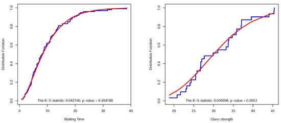
Figure 3. (Left): Empirical and fitted $AK(2,5,0.081045,0.202490)$ for data set of Example 1. (Right): Empirical and fitted $AK(13,4,0.707794,0.421921)$ for data set of Example 2.

As for the second data set, Fuller et al. [22] and Shanker [23] considered the strength of the glass of an aircraft window presented in Table 4. To find a suitable model for describing this data set, we fit $AK(\alpha ,\beta ,\delta ,\theta )$ for all pairs $(\alpha ,\beta )$ where $\alpha =1,2,\cdots ,15$ and $r=0,1,2,\cdots ,15$ to this data set. Then, we search for the model with the smallest AIC and/or K-S statistic and find $AK(13,4,0.707794,0.421921)$. The AIC, K-S statistic and its p-value are $214.2097$, $0.096998$ and $0.9053$, respectively. Figure 3, right side, shows the empirical CDF and fitted model $AK(13,4,0.707794,0.421921)$.

Table 4. Strength of glass of aircraft window, reported by Fuller [22].

18.83	20.8	21.657	23.03	23.23	24.05	24.321	25.5	25.52	25.8	26.69
26.77	26.78	27.05	27.67	29.9	31.11	33.2	33.73	33.76	33.89	34.76
35.75	35.91	36.98	37.08	37.09	39.58	44.045	45.29	45.381

Finally, Smith and Naylor [24] reported a data set of strength of 1.5 cm glass fibers presented in Table 5. This data set has also been analyzed by Shukla and Shanker [25]. Here we fit $PAK(\alpha ,\beta ,\delta ,\theta ,\gamma )$ to this data set for all pairs $(\alpha ,\beta )$ where $\alpha =1,2,\cdots ,10$ and $\beta =0,1,\cdots ,10$. Based on the AIC and K-S statistic the best model among them is $PAK(5,2,1.301490,0.795791,3.677124)$. The AIC, K-S statistic and its related p-value are $28.09806$, $0.084074$ and $0.764707$, respectively. The empirical CDF and the CDF of $PAK(5,2,1.301490,0.795791,3.677124)$ have been drawn in Figure 4.

Table 5. Strength of 1.5 cm glass fibers, analyzed in Example 3.

0.55	0.93	1.25	1.36	1.49	1.52	1.58	1.61	1.64	1.68	1.73
1.81	2.00	0.74	1.04	1.27	1.39	1.49	1.53	1.59	1.61	1.66
1.68	1.76	1.82	2.01	0.77	1.11	1.28	1.42	1.50	1.54	1.60
1.62	1.66	1.69	1.76	1.84	2.24	0.81	1.13	1.29	1.48	1.50
1.55	1.61	1.62	1.66	1.70	1.77	1.84	0.84	1.24	1.30	1.48
1.51	1.55	1.61	1.63	1.67	1.70	1.78	1.89

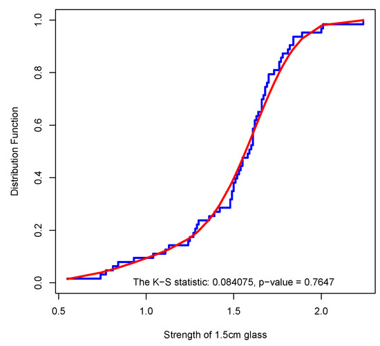
Figure 4. Empirical and fitted $PAK(5,2,1.301490,0.795791,3.677124)$ for data set of Example 3.

6. Conclusions

We have proposed a general extension of the Lindley model, namely, $AK(\alpha ,\beta ,\delta ,\theta )$, that includes many of the previous extensions. Moreover, we have introduced its power version, $PAK(\alpha ,\beta ,\delta ,\theta ,\gamma )$. Unlike the Lindley model, these extensions are scale invariant. Several statistical and reliability properties of the proposed models have been presented. The maximum likelihood estimator of the parameters has been simulated and studied for complete and right-censored data. The efficiency and the behavior of estimate have been, as well, investigated by a simulation study. Some real data sets have been analyzed and the results show that the proposed models are very flexible and useful in applications. As the applications show, we can search among all $\alpha$ and $\beta$ in a range and find the more suitable model. We hope that this model will be able to attract a wide spectrum practical studies in reliability engineering, survival analysis, and other fields of life. Further properties and applications of the new models can be considered in the future of this research. In particular, it is worth noting that when the Poisson parameter follows the $AK(\alpha ,\beta ,\delta ,\theta )$, the model leads to an interesting discrete model that is flexible and compliant for modeling other discrete-valued life problems. This topic is interesting and open problems remain.

References

- Tobias, P.A.; Trindade, D. Applied Reliability; CRC Press: Boca Raton, FL, USA, 2011; ISBN 9781584884668. [Google Scholar]
- Wolstenholme, L.C. Reliability Modelling: A Statistical Approach; Chapman and Hall/CRC: Boca Raton, FL, USA, 1999; ISBN 9781584880141. [Google Scholar]
- Schwartz, R. Biological Modeling and Simulation: A Survey of Practical Models, Algorithms, and Numerical Methods; MIT Press: Cambridge, MA, USA, 2008. [Google Scholar]
- McPherson, J.W. Reliability Physics and Engineering: Time-to-Failure Modeling; Springer US: New York, NY, USA, 2010; ISBN 978-1-4419-6348-2. [Google Scholar]
- Lindley, D.V. Fiducial distributions and Bayes’ theorem. J. R. Stat. Soc. Ser. B Methodol. 1958, 20, 102–107. [Google Scholar] [CrossRef]
- Ghitany, M.E.; Al-Mutairi, D.K.; Nadarajah, S. Zero-truncated Poisson-Lindley distribution and its application. Math. Comput. Simul. 2008, 79, 279–287. [Google Scholar] [CrossRef]
- Ghitany, M.E.; Al-Mutairi, D.K.; Awadhi, F.A.; Alburais, M. Marshall-Olkin extended Lindley distribution and its application. Int. J. Appl. Math. 2012, 25, 709–721. [Google Scholar]
- Bakouch, H.S.; Bander, M.A.; Al-Shaomrani, A.A. Marchi and F. Louzada, An extended Lindley distribution. J. Korean Stat. 2012, 41, 75–85. [Google Scholar] [CrossRef]
- Abouammoh, A.M.; Alshangiti Arwa, M.; Ragab, I.E. A new generalized Lindley distribution. J. Stat. Comput. Simul. 2015, 85, 3662–3678. [Google Scholar] [CrossRef]
- Cakmakyapan, S.; Ozel, G. The Lindley family of distributions: Properties an applications. Hacet. J. Math. Stat. 2017, 46, 1113–1137. [Google Scholar] [CrossRef]
- Shanker, R.; Mishra, A. A quasi Lindley distribution. Afr. J. Math. Comput. Sci. Res. 2013, 6, 64–71. [Google Scholar]
- Lai, C.D.; Xie, M. Stochastic Aging and Dependence for Reliability; Springer: New York, NY, USA, 2006; ISBN 978-0-387-29742-2. [Google Scholar]
- Shanker, R. Akash distribution and its applications. Int. J. Probab. Stat. 2015, 4, 65–75. [Google Scholar] [CrossRef]
- Shukla, K.K. Prakaamy distribution with properties and applications. JAQM 2018, 13, 30–38. [Google Scholar]
- Shanker, R. Shanker distribution and its applications. Int. J. Stat. Appl. 2015, 5, 338–348. [Google Scholar] [CrossRef]
- Shanker, R.; Shukla, K.K. Ishita distribution and its applications. Biom. Biostat. Int. J. 2017, 5, 39–46. [Google Scholar] [CrossRef]
- Shukla, K.K. Pranav distribution with properties and its applications. Biom. Biostat. Int. J. 2018, 7, 244–254. [Google Scholar] [CrossRef]
- Shukla, K.K. Ram Awadh distribution with properties and applications. Biom. Biostat. Int. J. 2018, 7, 515–523. [Google Scholar] [CrossRef]
- Fleming, T.R.; Harrington, D.P. Counting Processes and Survival Analysis; Wiley: Hoboken, NJ, USA, 2011; ISBN 978-1-118-15066-5. [Google Scholar]
- Ghitany, M.E.; Atieh, B.; Nadarajah, S. Lidley distribution and its application. Math. Comput. Simul. 2008, 78, 493–506. [Google Scholar] [CrossRef]
- Corder, G.W.; Foreman, D.I. Nonparametric Statistics: A Step-by-Step Approach, 2nd ed.; Wiley: Hoboken, NJ, USA, 2014; ISBN 978-1-118-84031-3. [Google Scholar]
- Fuller, E.J.; Frieman, S.; Quinn, J.; Quinn, G.; Carter, W. Fracture mechanics approach to the design of glass aircraft windows: A case study. SPIE Proc. 1994, 2286, 419–430. [Google Scholar]
- Shanker, R. On Generalized Lindley Distribution and Its Applications to Model Lifetime Data from Biomedical Science and Engineering. 2016. Available online: https://biomedicine.imedpub.com/on-generalized-lindley-distribution-and-its-applications-to-model-lifetime-data-from-biomedical-science-and-engineering.php?aid=17803 (accessed on 25 November 2016).
- Smith, R.L.; Naylor, J.C. A comparison of maximum likelihood and Bayesian estimators for the three parameter Weibull distribution. Appl. Stat. 1987, 36, 358–369. [Google Scholar] [CrossRef]
- Shukla, K.K.; Shanker, R. Power Prakaamy distribution and its applications. Int. J. Comp. Theo. Stat. 2020, 7. [Google Scholar] [CrossRef]
Publisher’s Note: MDPI stays neutral with regard to jurisdictional claims in published maps and institutional affiliations. |
© 2020 by the authors. Licensee MDPI, Basel, Switzerland. This article is an open access article distributed under the terms and conditions of the Creative Commons Attribution (CC BY) license (http://creativecommons.org/licenses/by/4.0/).