Abstract
This paper proposes a method for learning the process of curve fitting through a general class of totally positive rational bases. The approximation is achieved by finding suitable weights and control points to fit the given set of data points using a neural network and a training algorithm, called AdaMax algorithm, which is a first-order gradient-based stochastic optimization. The neural network presented in this paper is novel and based on a recent generalization of rational curves which inherit geometric properties and algorithms of the traditional rational Bézier curves. The neural network has been applied to different kinds of datasets and it has been compared with the traditional least-squares method to test its performance. The obtained results show that our method can generate a satisfactory approximation.
1. Introduction
The problem of obtaining a curve that fits a given set of data points is one of the fundamental challenges of Computer Aided Geometric Design (CAGD), and it has become prevalent in several applied and industrial domains, such as Computer-Aided Design and Manufacturing (CAD/CAM) systems, Computer Graphics and Animation, Robotics Design, Medicine and many others. To face this issue, several families of bases of functions have been considered. There is a large body of literature on this topic and there are numerous methods to solve this issue, such as several least-squares techniques and different progressive iterative approximation methods (see [1,2,3] and the references therein).
Given a system of linearly independent functions defined on an interval and , we can define a parametric curve as , . The polygon , formed by the ordered sequence of points , , is called the control polygon of γ and the points , , are named the control points of with respect to . A matrix is totally positive (TP) if all its minors are nonnegative (see [4]). A system of functions defined on I is TP if all its collocation matrices with in I are TP. A TP system of functions on I is normalized (NTP) if , for all . A basis provides shape-preserving representations if the shape of the curve imitates the shape of its control polygon. Normalized totally positive bases provide shape-preserving representations. The normalized B-basis of a given space is an NTP basis such that the matrix of change of basis of any NTP basis with respect to the normalized B-basis is TP and stochastic. This property implies that the control polygon of a curve with respect to the normalized B-basis can be obtained by a corner cutting algorithm from its control polygon with respect to any other NTP basis. Thus, the control polygon with respect to the normalized B-basis is closer in shape to the curve than the control polygon with respect to any other NTP basis. Furthermore, the length of the control polygon with respect to the normalized B-basis lies between the length of the curve and the length of its control polygon with respect to any other NTP basis. Similar properties hold for other geometric properties such as angular variation or number of inflections (see [5,6,7]). So, the Normalized B-basis has the optimal shape-preserving properties among all NTP bases of the space. The Bernstein bases and the B-spline bases are the normalized B-bases of their corresponding generated spaces.
It is well known that the bases obtained by rationalizing Bernstein bases are also the normalized B-bases of the generated spaces of rational functions. These spaces are made up of rational polynomial functions where the denominator is a given polynomial. Rational Bernstein bases add adjustable weights to provide closer approximations to arbitrary shapes and have become a standard tool in CAGD since they allow the exact representation of conic sections, spheres and cylinders. In [8], the generalization of rational Bernstein bases obtained when replacing the linear polynomial factors by trigonometric or hyperbolic functions or their mixtures with polynomials were analyzed. The generated rational curves inherit geometric properties and algorithms of the traditional rational Bézier curves and so, they can be considered as modeling tools in CAD/CAM systems.
As mentioned before, the weights of rational bases can be used as shape parameters. However, it is well known that the effect of changing a weight in a rational basis is different from that of moving a control point of the curve (see Figure 1). Thus, the interactive shape control of rational curves through adjusting weights is not a straightforward task and it is not easy to design algorithms to obtain the appropriate weights (see [9], Chapter 13).

Figure 1.
Initial curve (line) and curve obtained (dotted line) after changing the weights and/or control points. Left: changing the fourth weight; center: changing the fourth control point; and right: changing the fourth weight and the fourth control point.
Some recent papers have shown that the application of Artificial Intelligence (AI) techniques can achieve remarkable results regarding the problem of obtaining rational curves that fit a given set of data points. To face this issue, in [10], a bio-inspired algorithm was applied through the use of rational Bézier curves. Besides, in [11,12], evolutionary algorithms were applied to rational B-spline curves. As a novelty, in this paper, we define a one-hidden-layer neural network using the general class of rational bases with optimal shape-preserving properties proposed in [8]. In that work, the authors presented evaluation and subdivision algorithms. However, this is the first time that the problem of obtaining a rational fitting curve using these general class of totally positive rational bases is modeled by a neural network and its weights and control points optimized using a training algorithm. In this paper, we extend [8] for their application in curve fitting training the neural network with a recent stochastic learning process, the AdaMax algorithm [13], to find suitable weights and control points. In this approximation process, the rational basis is a hyperparameter and can be changed by substituting the linear factors by polynomial, trigonometric or hyperbolic functions, thus expanding the potential range of applications to include more difficult shapes.
The layout of the paper is as follows. In Section 2, we recall several concepts regarding CAGD and we present a general class of rational bases which are normalized B-bases. Then, in Section 3, we present a one-hidden-layer neural network based on the rational bases presented in the previous section to approximate a given set of data points. This neural network is trained with an optimization algorithm to update the weights and control points used to construct a curve that approximates the given set of data points, while decreasing a loss function. In Section 4, several experiments are provided illustrating the use of the neural network with different normalized B-bases to test its performance giving an approximation of different kinds of sets of data points. Moreover, the proposed method has been compared with the traditional least-squares method. Finally, conclusions and future work are presented in Section 5.
2. Shape-Preserving and Rational Bases
Let us suppose that and are nonnegative continuous functions. Then, for , we can define the system where:
For any positive weights , , let us define and denote by the rational basis described by
where is defined in (1). Clearly, this system spans a space of rational functions with denominator ,
where is the space generated by .
The following result corresponds to Corollary 4 of [8] and provides the conditions characterizing that the system given in (2) has optimal shape-preserving properties.
Proposition 1.
Let us see several choices of functions f and g satisfying the conditions of Proposition 1. Let us consider the functions
It is well known that the corresponding rational basis (2), which is the rational Bernstein basis, is the normalized B-basis of its generated space (3).
We can also consider the functions
The corresponding rational basis (2) spans the space
where the system given in (1) spans the space of even polynomials defined on of degree less than or equal to .
Trigonometric and hyperbolic bases are attracting a lot of interest, for instance in Isogeometric Analysis (cf. [14]). Let . Define
Let us notice that the functions f and g satisfy and for all . Moreover, it can be checked that
Therefore, for any , the function is a strictly increasing function on and f and g satisfy the conditions of Proposition 1. The corresponding rational basis (2) spans the space
where, for a given , the system given in (1) is a basis that coincides, up to a positive scaling, with the normalized B-basis of the space of trigonometric polynomials of degree less than or equal to m on I (see Section 3 of [15]).
Finally, let . Define
Clearly, and for all . Moreover, it can be checked that
Therefore, for any , is a strictly increasing function on and f and g satisfy the conditions of Proposition 1. The corresponding rational basis (2) spans the space
where, for , the system given in (1) spans the space of hyperbolic polynomials of degree less than or equal to m on I.
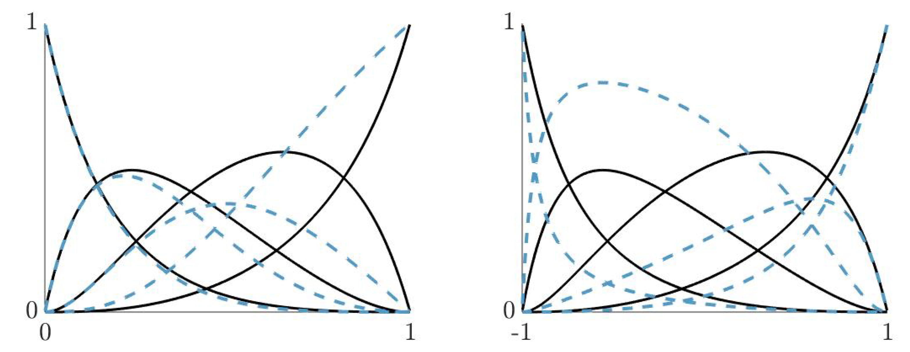
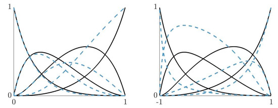
In Figure 2, we illustrate two examples of the rational basis (2) of degree 3. Let us observe the effect on the shape of the functions of the basis as weights change.
Section 4 will show examples of approximations of given sets of data points using all the above mentioned normalized B-bases. Moreover, the neural network presented in the following section will be used to compute the optimal weights and control points of their corresponding fitting curves.
3. Curve Fitting with Neural Networks
It is well known that curve fitting is the process of constructing a curve, or mathematical function, that has the best fit of a given set of data points. A related topic is Regression Analysis in Machine Learning. In the literature (see [16] (Chapter 11)), a regression problem is the problem of predicting a real value for each input data. Let us consider an input space and target values , and a distribution over , denoted by . Then, a regression problem consists of a set of labeled samples drawn according to where are the target real values we want to predict. There exists a huge variety of regression algorithms, i.e., algorithms solving regression problems, such as Linear Regression, Decision Trees, Support Vector Regression, and Neural Networks, among others. The quality of the prediction of an algorithm or model depends on the difference between the target (i.e., the true value) and the predicted one, and it is measured using a loss function. Then, given a set (also called “hypothesis”) of function mappings X to Y, the aim of the regression algorithm is to use S to find such that the expected loss is small.
Specifically, the problem that we want to solve can be stated as follows. Suppose that f and g are functions defined on satisfying the conditions of Proposition 1. Consider a set of parameters and a sequence of data points , where each parameter is associated with a data point . For some , we want to obtain a rational curve
to approximate the set of data points . Therefore, the goal is to obtain the weights and the control points of the rational curve (11) that best fits the set of data points. In order to compute them, we have used a stochastic optimization process to train a neural network that models the rational curve .
The problem to be solved can be interpreted then as a regression problem where the set of labeled samples is composed of the input data, X, that is the set of parameters and the target set of data points .
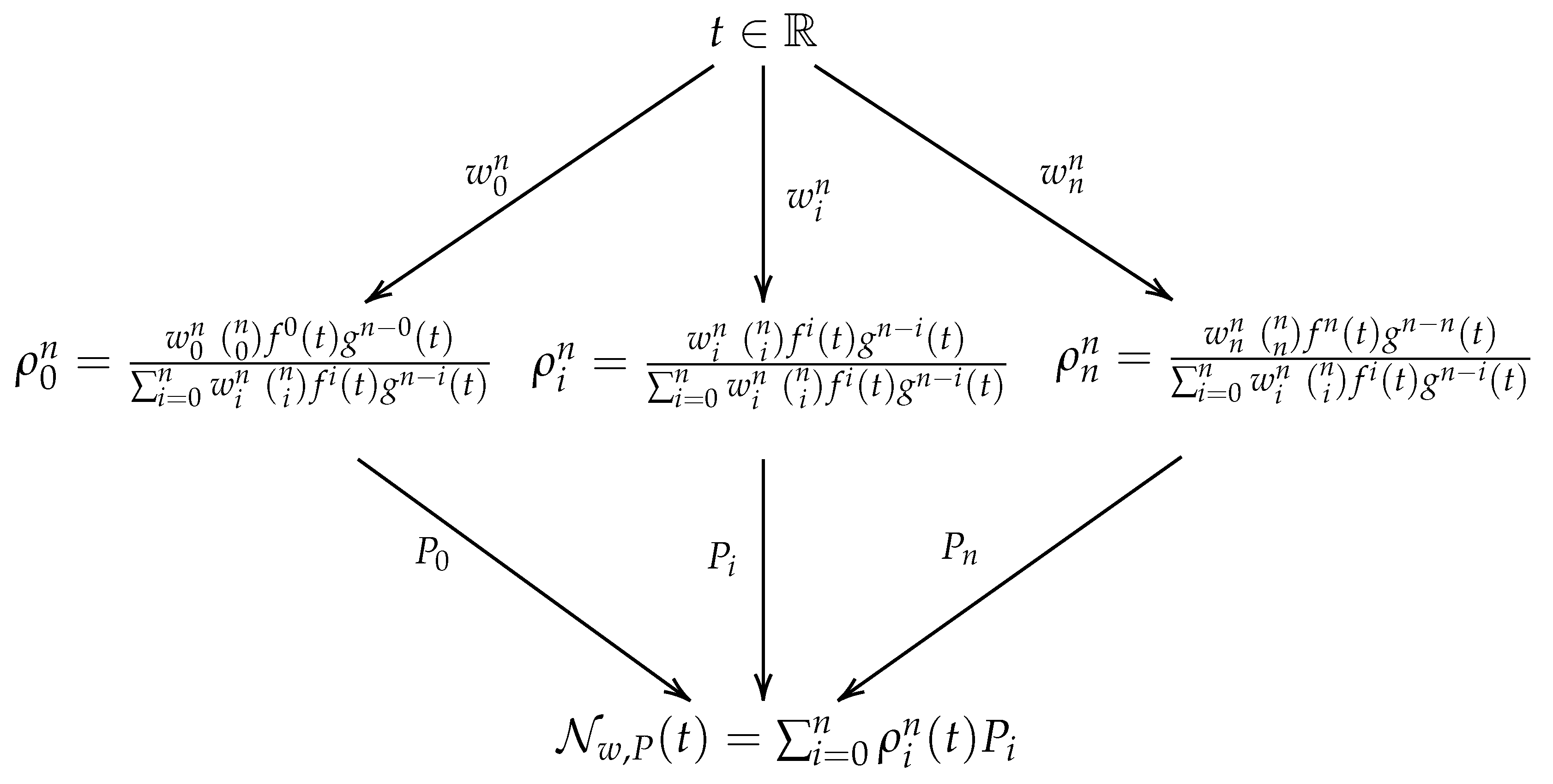
Then, the expression in (11) can be represented as a hierarchical computational graph with just one hidden layer that we will denote as where the computations are organized as in Figure 3. The obtained curve is the rational curve that approximates the given set of data points and we denote as the fitting curve.
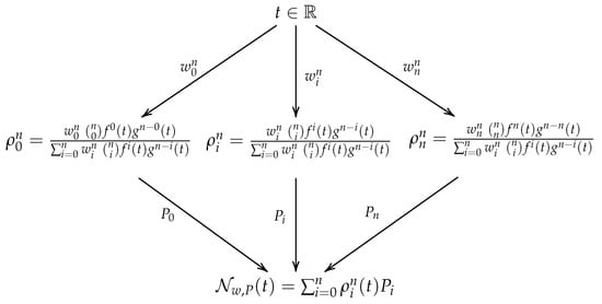
Figure 3.
From top to bottom. The input layer has the parameter as input. The hidden layer is of width and its parameters are the weights. Then, the output layer computes the approximation of the target curve and its parameters are the control points.
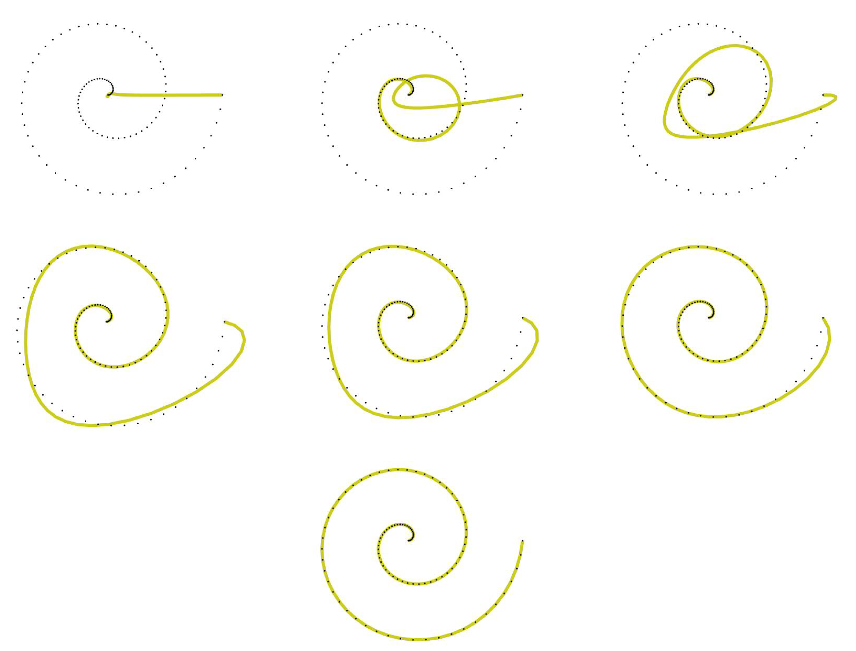
The key idea is to iteratively change the input weights and control points of the active curve , and so it deforms towards the target shape represented by the set of data points (see Figure 4).

Figure 4.
Evolution of the fitting curve . Set of data points from the target curve (dotted) and the fitting curve (line). From top to bottom and left to right: Increment , , , , , and .
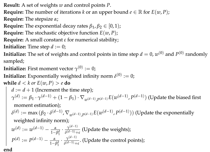
Then, we apply an adaptive learning rate optimization algorithm to train the neural network to find the weights and control points, which can be, for example, the Adaptive Moment Estimation (Adam) algorithm or its variant Adaptive Moment Estimation Maximum (AdaMax) algorithm based on infinity norm. These methods are used for stochastic optimization, to solve the supervised learning problem and to find the parameters where a minima is located. In this paper, we have mainly used the AdaMax variant (see Algorithm 1) because of its stability and simplicity [13]. However, the Adam method can be useful depending on the shape of the set of data points to be approximated and the choice of the loss function. The stochastic objective function, also called the loss function, measures the goodness of the fitting curve. Let us notice that there exist different loss functions such as the mean absolute error, the cross-entropy loss, the mean squared error, among others (the different loss functions implemented in Tensorflow can be consulted in the tensorflow documentation), that can be chosen depending on the problem. In our case, we have considered the mean absolute error as the loss function because of the choice of the training algorithm, given by the following expression:
The Adam and the AdaMax algorithms are stochastic gradient-based optimization algorithms and, as previously mentioned, they update the weights and the control points iteratively. The step size is a real number that measures how much the weights and the control points are updated upon each iteration. Besides, the Adam algorithm uses the first and the second moment estimate to update the weights and the control points which are updated following exponential decay rates ( and ). Finally, as AdaMax is a variation of Adam using infinity norm, the second moment estimate has a simple recursive formula which will be denoted in Algorithm 1 as exponentially weighted infinity norm. See [13] for a detailed description of the both Adam and AdaMax algorithms.
| Algorithm 1: The AdaMax algorithm [13] adapted to our context. |
 |
The number of units (i.e. weights and control points) is a hyperparameter and is determined based on the complexity of the shape to be approximated. Besides, the step size, , can be changed depending on the state of the convergence of the training procedure, for example, when the loss values (i.e., the evaluation of the loss function) gets stuck or the update of the parameters is too big. Then, it is useful to increase or reduce, respectively, the step size according to the values of the loss function.
4. Experiments Results
In order to show the performance of the neural network , we have taken different sets of data points . They have been chosen to reflect the variety of situations where the proposed neural network can be applied. The first set of data points belongs to a closed conic curve, the second one belongs to a transcendental curve, the third one is a curve with a twisted shape and, finally, the fourth one is a noisy set of data points from a baroque image.
In all cases, we have taken different functions f and g satisfying the conditions of Proposition 1 and allowing that the corresponding rational bases (2) have the optimal shape-preserving properties.
Remark 1.
One of the requirements for a rational basis to be the normalized B-basis of its generated space is the positivity of the weights. This makes it necessary to apply the absolute value to the weights in the weight update step of Algorithm 1. However, in the experiments shown, we opted to avoid this choice because we have observed that, although in the intermediate steps the weights could be negative, at the end of the training, the weights were positive and the convergence was faster. Nevertheless, we can add the restriction depending on the needs.
Let us notice that we have used an uniform distribution of the parameters , , in all the examples. This choice of parameters does not have to be the optimal but we have preferred it because of its simplicity. Besides, a normalization of the data points, , between 0 and 1, was applied in order to facilitate the training procedure following the formula:
The AdaMax algorithm was applied to solve the minimization problem with the mean absolute error loss function (12) with the following choice of hyperparameters: . Then, the number of iterations of the algorithm depends on the desired accuracy of the fitting curve to the set of data points. In this case, we have used between 3000 to 5000 iterations of the algorithm but, with more iterations and a better tuning of the parameters, the results provided here may be improved. Finally, in order to reach a better approximation, the first and the last control point of the fitting curve were fixed to be the same as the first and the last point of the set of data points, thus the obtained fitting curve is always exactly at those points. We can see in Table 1, a summary of the loss values from different fitting curves. Let us observe that the value n is the degree of the fitting curve and it depends on the complexity of the shape to be approximated. Moreover, let us notice that the proposed neural network is able to obtain a suitable accuracy with low degrees and, as a generalization of other methods, we can choose, depending on the shape of the set of data points, the basis that best fits. Note that, in CAGD, it is important to properly address the problem of curve fitting, finding a balance between accuracy and degree of the curve since high-degree curves are computationally expensive to evaluate. The AdaMax algorithm has been selected because it is computationally efficient with little memory requirements, suited for problems with large data or parameters. In Table 2, the time of execution of the Algorithm 1 using different numbers of units (i.e., weights and control points) and numbers of iterations is provided.

Table 1.
Loss values of the mean absolute error (12) for different fitting curves of degree n with , , (Basis 1), and , , (Basis 2), and , , , , (Basis 3) and finally and , , , (Basis 4). They were all trained with 4000 iterations, , , , . The process was repeated 5 times, with the loss values provided being the best values reached.

Table 2.
Time of execution of the proposed algorithm measured in seconds for different numbers of units and iterations. The values provided are the mean of 5 repetitions with a set of data points of size 100.
The implementation (the code of the experimentation can be found in https://github.com/Cimagroup/Curve-approximation-NN) was developed using TensorFlow 2.0 [17] allowing developers to easily use it to build and deploy Machine Learning powered applications. All experiments were ran on a Quad-Core Intel Core i7 CPU, 2.8 GHz with 16 GB RAM. Let us see a detailed description of the experiments.
4.1. Circle Curve
Circles and conic sections play a relevant role in curve design and have been approximated in several works (see [18,19]). Let us show different approximations to the circle given by the parametric equations
. First, let us see an approximation obtained performing the neural network using polynomial functions.
We have taken the following sequence of points on the circle (14):
being the parameters , .
For , we have approximated the set s by the fitting curve considering the functions and at the vector nodes with as above. After training the neural network , performing the Algorithm 1 for 3000 iterations, we have obtained the following weights:
and the following control points:
We can see in Figure 5 the obtained fitting curve of degree 5 and its corresponding control polygon.
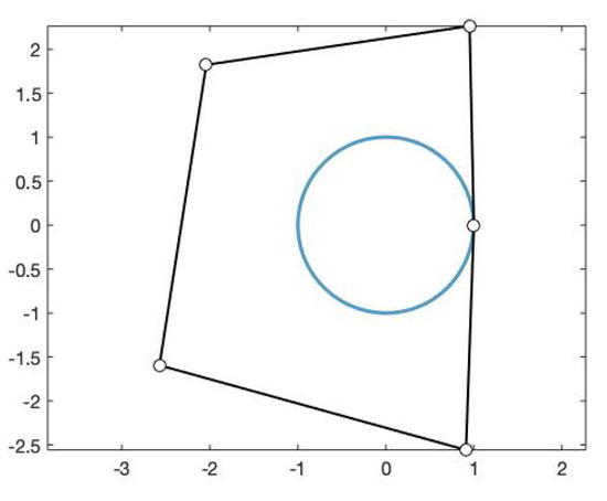
Figure 5.
Fitting curve of degree 5 obtained using the functions and , , and its corresponding control polygon.
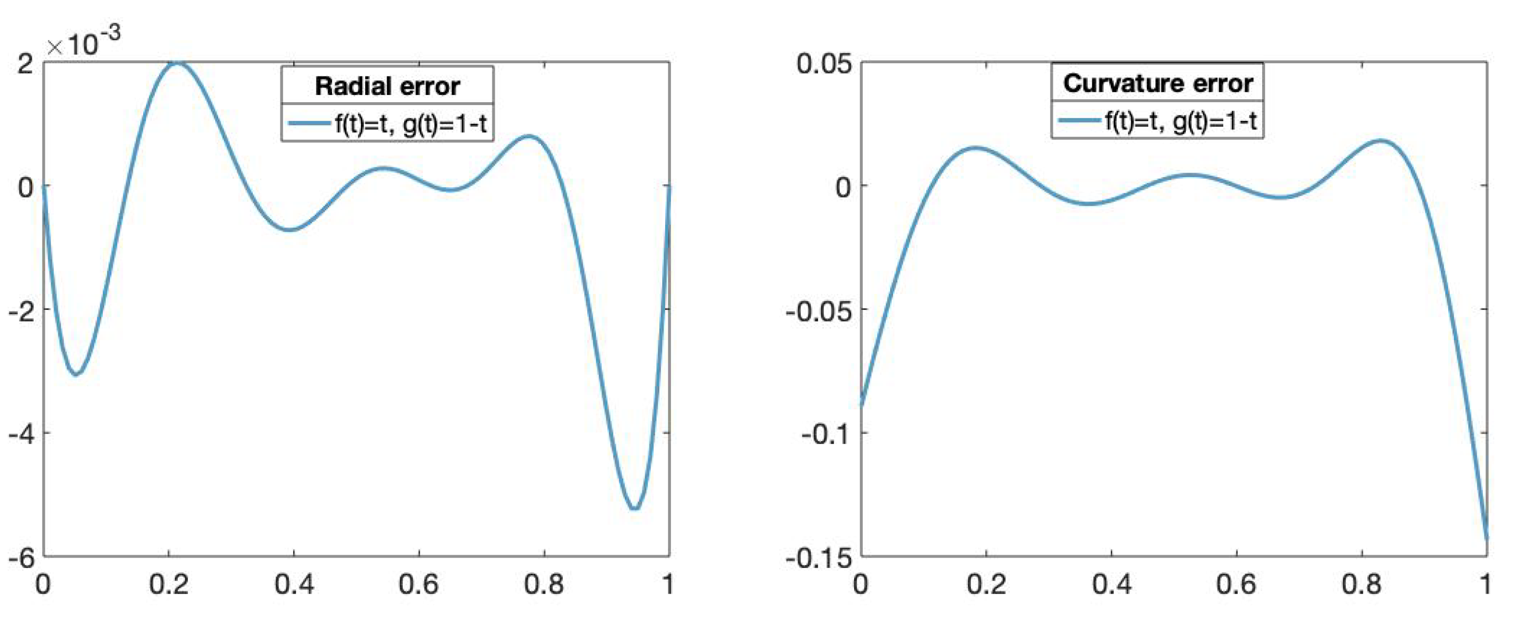
In order to analyze the performance of the obtained approximation to the circle, we depict some geometric approximations of the approximation error. In Figure 6, we plot the radial and curvature errors given, respectively, by
where and .

Figure 6.
(Left): The x-axis represents the parameters t in and the y-axis represents the radial error value of the fitting curve obtained using the functions and , . (Right): The x-axis represents the parameters t in and the y-axis represents the curvature error value of fitting curve obtained using the functions and , .
We can observe that the radial error vanishes at because the approximation is exact for the initial and the last points of the curve.
Let us see another approximation example of the unit circle performing the neural network using trigonometric functions. We have the following set of data points on circle (14):
being the parameters , , with . For , we have approximated the set s by the fitting curve using the functions and at the vector nodes with as above. After training the neural network , performing Algorithm 1 for 3000 iterations, and with , we have obtained the following weights:
and the following control points:
We can see in Figure 7 the fitting curve of degree 5 obtained and its control polygon.
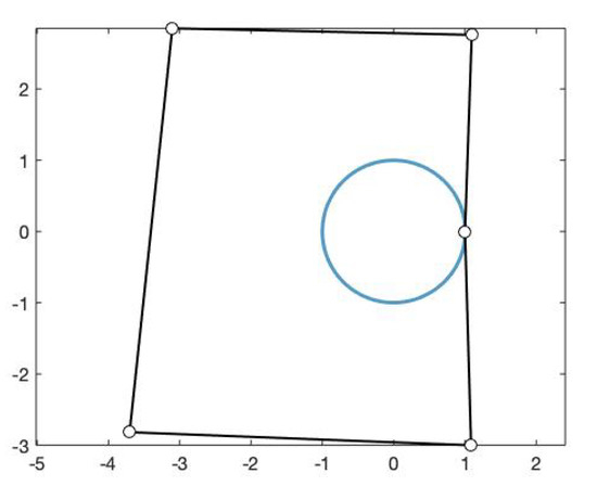
Figure 7.
Fitting curve of degree 5 using and , , and its control polygon.
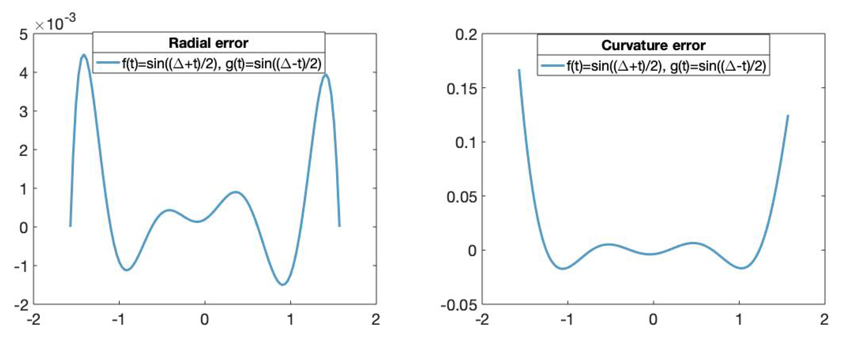
Figure 8 shows its corresponding radial and curvature errors. We can observe that the radial error vanishes at because the approximation is exact for the initial and the last points of the curve.
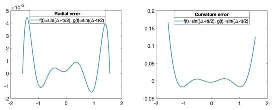
Figure 8.
(Left): The x-axis represents the parameters t in and the y-axis represents the radial error value of the fitting curve obtained using the trigonometric basis. (Right): The x-axis represents the parameters t in and the y-axis represents the curvature error value of the fitting curves obtained using the trigonometric basis.
Finally, for different values of n, Figure 9 shows the history of the loss function given in (12) through the training process on 3000 iterations of the neural network using the polynomial functions and the trigonometric functions. We can observe, in both cases, that the convergence to the circle of the fitting curves is faster as n increases.

Figure 9.
For different values of n, the history of the loss function, i.e., the mean absolute error values, through the training process on 3000 iterations while the fitting curves converges. (Left): Loss values of the fitting curve using , , . (Right): Loss values of the fitting curve using , , . The x-axis represents the iteration of the training algorithm and the y-axis represents the mean absolute error value.
4.2. Cycloid Curve
Cycloids are commonly used in manufacturing applications (e.g. gear tooth geometry). The cycloid is a transcendental curve and thus, it cannot be expressed by polynomials exactly. Creating a complex curve in a CAD/CAM system is not always straightforward. In [20], it is shown the need to new methods for approximating this curve. Let us show different approximations to the cycloid by several fitting curves obtained by training the neural network using polynomial, trigonometric and hyperbolic functions f and g that satisfy the conditions of Proposition 1.
The cycloid is given by the parametric equations
. We have taken the following sequence of points on the cycloid (15):
being the parameters , .
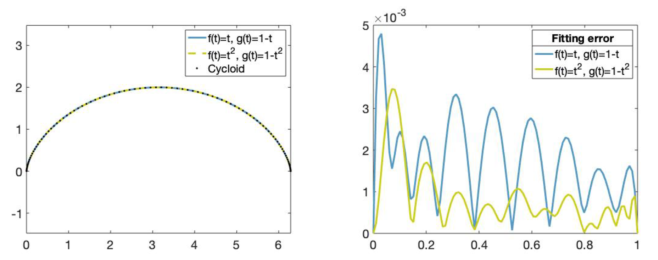
For , we have approximated the set s by two fitting curves at the vector nodes with as above. One of the fitting curves is obtained using the functions and , and the other fitting curve is obtained using the functions and .
We can see in Figure 10, the fitting curves and their corresponding fitting error. The fitting error is given by the Euclidean norm between the approximated curve—in this case, the cycloid curve—and the obtained fitting curve. Observe that the cycloid curve is better approximated by the fitting curve obtained using the functions and than by the fitting curve obtained using the functions and .

Figure 10.
(Left): Set of data points on the cycloid (dotted), fitting curve obtained using the functions , , (blue) and fitting curve obtained using the functions ,, (green). (Right): Fitting error comparison.The x-axis represents the parameters t in and the y-axis represents the fitting error value of the fitting curves obtained using the functions , , (green) and the functions , , (blue).
Let us see two more approximations of the cycloid. We have taken the following sequence of points on the cycloid (15):
being the parameters , , with .
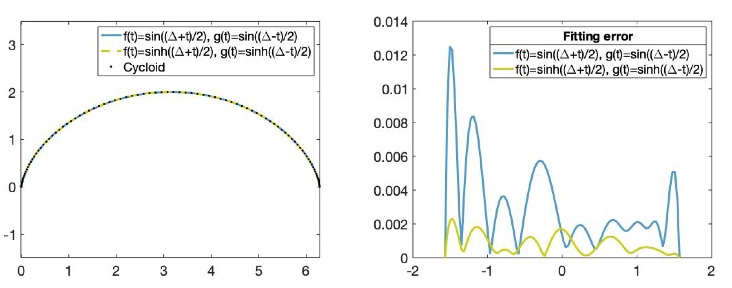
For , we have approximated the set s by two fitting curves at the vector nodes with as above. One of the fitting curves is obtained by training the neural network using the trigonometric functions and and the other one using the hyperbolic functions and .
We can see in Figure 11, the fitting curves and their corresponding fitting error. Let us observe that the cycloid is better approximated by the fitting curve obtained using the hyperbolic functions than the fitting curve obtained using the trigonometric functions.
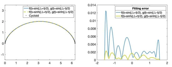
Figure 11.
(Left): Set of data points on the cycloid (dotted), fitting curve obtained using the trigonometric functions and and fitting curve obtained using the hyperbolic functions and . (Right): Fitting error comparison. The x-axis represents the parameters t in and the y-axis represents the curvature error value of the fitting curve obtained using the trigonometric and hyperbolic bases.
4.3. Archimedean Spiral Curve
Finally, let us show different approximations of the Archimedean spiral given by the parametric equations
First, let us see an approximation obtained training the neural network using polynomial functions. We have taken the following sequence of points on the Archimedean spiral (16):
being the parameters , .
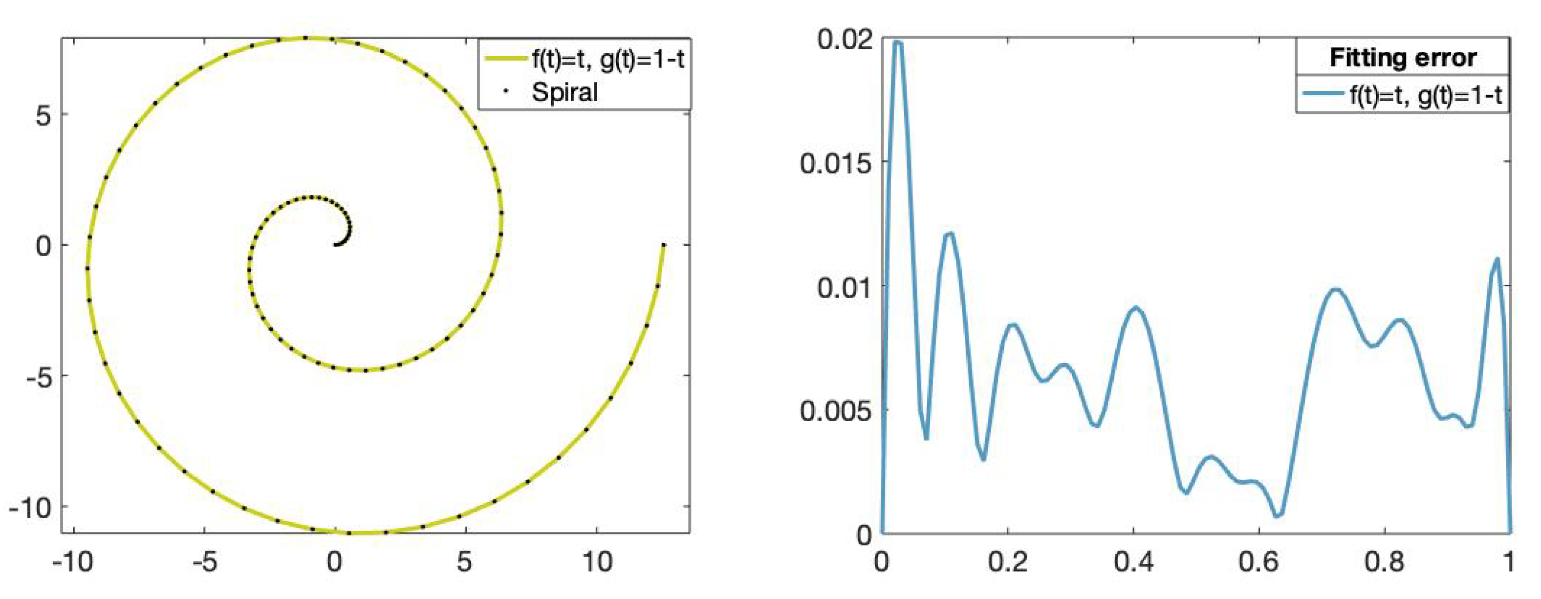
For , we have approximated the set s by the fitting curve using the functions and at the vector nodes with as above. Figure 12 shows the fitting curve of degree 11 and its corresponding fitting error.
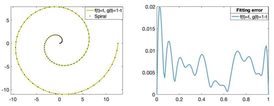
Figure 12.
(Left): Set of data points on the Archimedean spiral (dotted) and the fitting curve of degree 11 obtained using the functions and , . (Right): The x-axis represents the parameters t in and the y-axis represents the fitting error value of the fitting curve obtained using the functions and .
Let us see other examples in which the Archimedean spiral is approximated by the neural network using hyperbolic functions. We have taken the following sequence of points on the Archimedean spiral (16):
being the parameters , . For , we have approximated the set s by the fitting curve using the functions and at the vector nodes with as above.
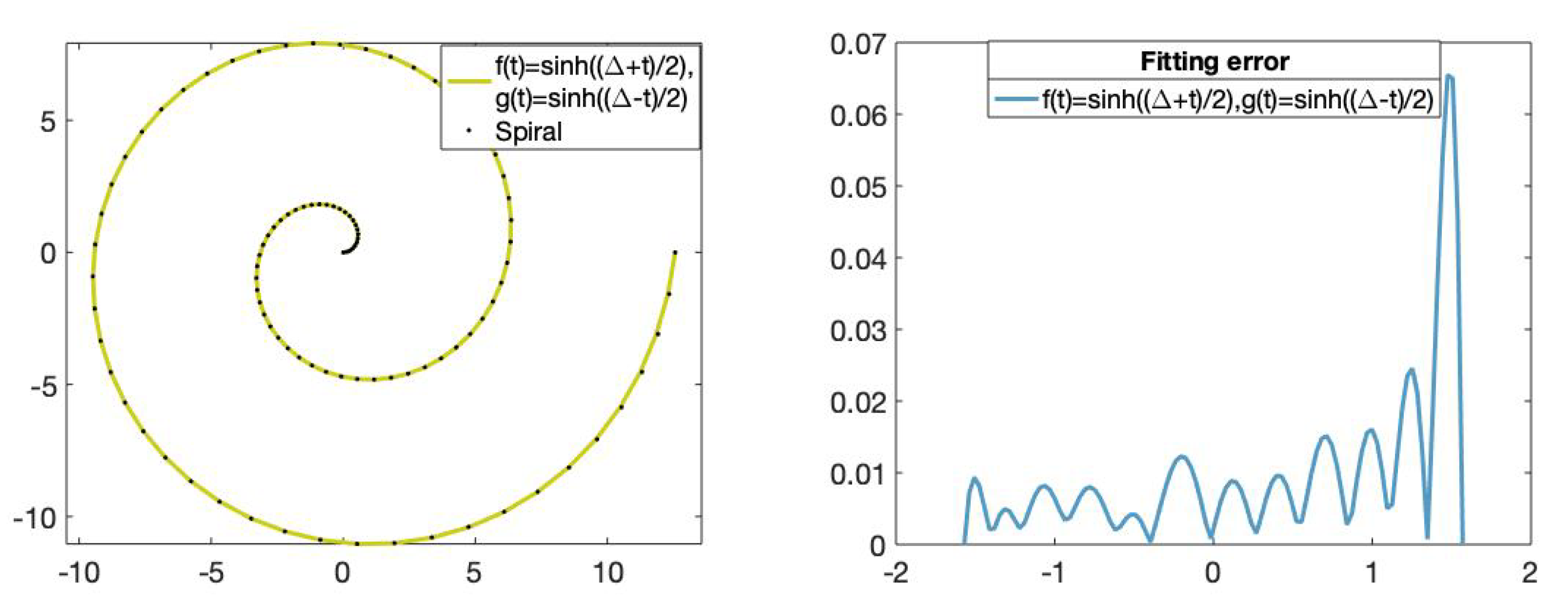
Figure 13 shows the fitting curve of degree 11 and its corresponding fitting error.
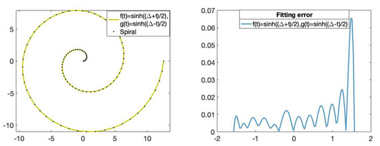
Figure 13.
(Left): Set of data points on the Archimedean spiral (dotted) and the fitting curve of degree 11 with the functions and . (Right): The x-axis represents the parameters t in and the y-axis represents the fitting error value of the fitting curve obtained using the hyperbolic basis.
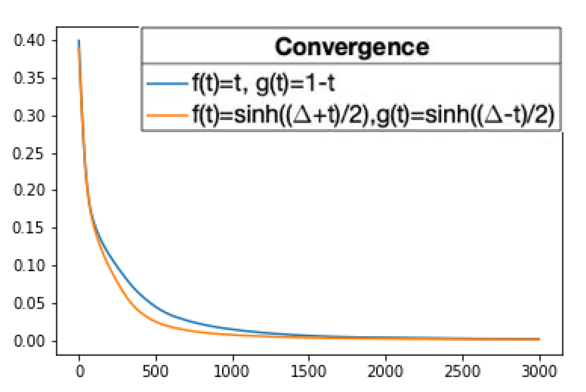
We can see in Figure 14, the convergence of the two above fitting curves. Let us observe that the fitting curve corresponding to the hyperbolic rational basis has a faster convergence. Therefore, once again, it seems that the choice of the functions f and g, hence the choice of the rational basis, is relevant to the approximation.
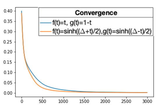
Figure 14.
The history of the loss values, i.e., the mean absolute error values, through 3000 iterations of the training algorithm while the fitting curves converge is pictured. The blue line corresponds to the fitting curve of degree 11 obtained using and , , and the orange line corresponds to the fitting curve of degree 11 obtained using and . The x-axis represents the iteration of the training algorithm and the y-axis represents the mean absolute error value. The values are the mean of 50 repetitions.
4.4. Comparison of Least-Squares Fitting and the Neural Network
In this section, the proposed neural network is compared with the least-squares method and the regularized least-squares method. It is well known that least-squares fitting is a common procedure to find the best fitting curve to a given set of data points by minimizing the sum of the squares of the data points from the curve ([9,21,22]). The least-squares method is sensitive to small perturbations in data and, in those cases, regularization methods can be applied such as the regularized least-squares method (see [23]). Therefore, two experiments have been developed. The set of data points used in the first experiment is a non-noisy parametrization of known curves, so the least-squares method has been applied. In the second experiment, we used an image to obtain a noisy set of data points and applied the regularized least-squares method.
The problem that we want to solve is stated as follows. Suppose that f and g are functions defined on satisfying the conditions of Proposition 1. Consider a set of parameters and a sequence of data points , where each parameter is associated with a data point . For some , we want to compute a rational curve
minimizing the sum of the squares of the deviations from the set of data points , that is, . In order to compute the control points of the fitting curve, we have to solve, in the least-squares sense, the overdeterminated linear system , where the matrix A is
In this fourth experiment, let us see two examples comparing the fitting curves obtained applying this traditional method and the fitting curves obtained by training the neural network . We have seen previously an approximation of the circle (14) obtained with the neural network for using the polynomial functions and , . Besides, we have seen an approximation of the Archimedean spiral (16) obtained with the neural network for using the polynomial functions and , . Using the same parameters and sets of data points, we solved the corresponding overdeterminated linear systems to obtain the control points of the curve that best fits the given data points in the least-squares sense. For this purpose, following the steps shown in Section 6.4 of [1], we have obtained the solutions of , firstly, by using the Matlab command SVD and, secondly, by using the Matlab command mldivide.
Since the weights are unknown and are necessary for solving the linear system in the least-squares sense, these have been randomly chosen within a positive range. Let us observe that one of the advantages of the neural network with respect to the least-squares method is that the neural network not only finds suitable control points, but it also finds suitable weights to fit the given set of data points.
In Table 3, the execution time of the least-squares method using a different number of weights and control points is provided. We can see that, although for low-degree fitting curves, the least-squares method is faster than the method proposed in this paper, for the fitting curves of degree greater than , the proposed method is faster than the least-squares method.

Table 3.
For different number of weights and control points, the time of execution of the least-squares method using the Matlab commands mldivide and SVD, and the time of execution of the Algorithm 1 for 3000 iterations are provided. The values have been measured in seconds with a set of data points of size 100 and they are the mean of 5 repetitions.
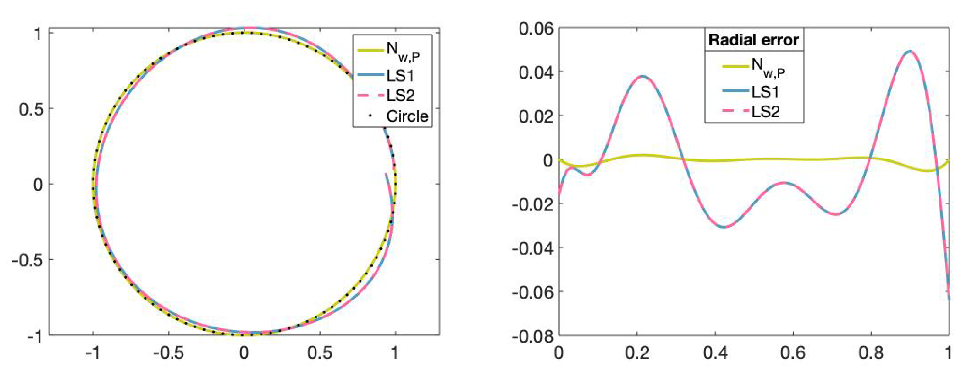
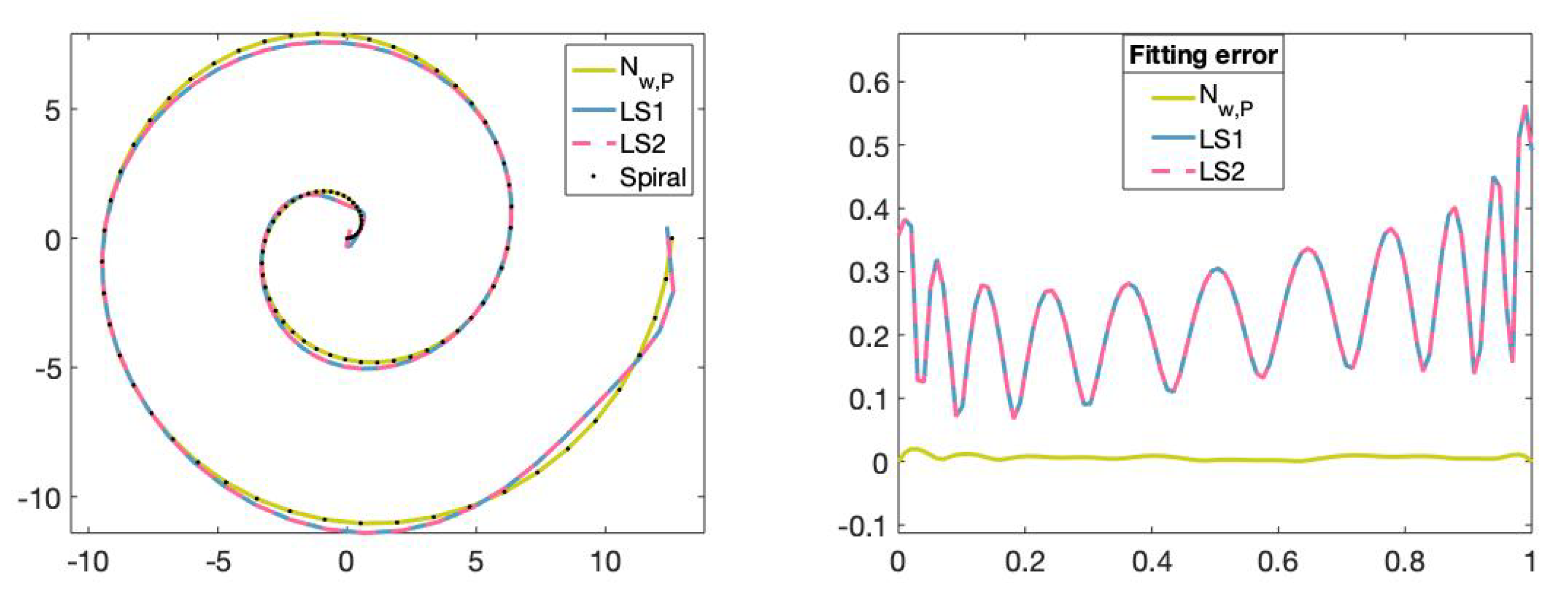
We can see in Figure 15 and Figure 16 that the fitting curves obtained by training the neural network are more accurate than the fitting curves obtained by applying the traditional least-squares method.
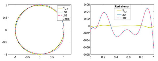
Figure 15.
(Left): Set of data points on circle (dotted), fitting curve of degree 5 obtained with the neural network, fitting curve of degree 5 obtained with the least-squares method by using the Matlab commmand mldivide (LS1), fitting curve of degree 5 obtained with the least-squares method by using the Matlab command SVD (LS2). (Right): The x-axis represents the parameters t in and the y-axis represents the radial error value of the fitting curves obtained with the different methods.
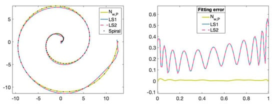
Figure 16.
(Left): Set of points on the Archimedean spiral curve, fitting curve of degree 11 obtained with the neural network, fitting curve of degree 11 obtained with the least-squares method by using the Matlab command mldivide (LS1) and fitting curve of degree 11 obtained with the least-squares method using the Matlab command SVD (LS2). (Right): The x-axis represents the parameters t in and the y-axis represents the fitting error value of the fitting curves obtained with the different methods.
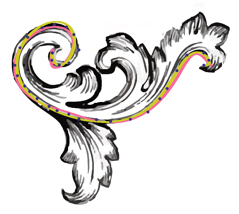
In the last experiment, we have taken 31 points from a baroque image as a set of data points (see Figure 17). We have approximated them by two fitting curves of degree 8 with hyperbolic functions at the vector nodes , such that , . The first fitting curve was obtained by training the neural network during 1000, reaching a final mean absolute error on the set of data points of . Besides, this example shows the robustness of the proposed method to noisy data points. The second fitting curve was obtained with random vector weights and the regularized least-squares method by using an adaptation of the Matlab library available in [24]. This last fitting curve reached a mean absolute error of . Visually, in Figure 17, it is appreciated that the fitting curve obtained by training the neural network achieves better curvature than the regularized least-squares method (which is more evident at the beginning and at the end of the curve). Finally, we would like to highlight that we have observed in all the executed experiments a good performance of the neural network for small values of n, in spite of the complexity of the set of data points.

Figure 17.
Noisy set of data points obtained from the baroque image (points in blue), fitting curve obtained by training the proposed neural network (points in green) and fitting curve obtained using the regularized least-squares method (pink). Baroque motif image source: Freepik.com.
5. Conlusions and Future Work
In this work, we have tackled the problem of finding a rational curve to fit a given set of data points. To solve this issue, we have proposed a one-hidden-layer neural network based on a general class of totally positive rational bases belonging to spaces mixing algebraic, trigonometric and hyperbolic polynomials, thus expanding the potential range of applications to include more difficult shapes. In order to obtain the weights and control points of the rational curve to fit the data points, the neural network is trained with an optimization algorithm to update the weights and control points while decreasing a loss function. The fitting curves of the numerical experiments show that for certain curves, the use of particular rational bases provides better results.
In future work, we wish to extend the neural network to obtain a suitable parametrization of the data points. The choice of the parameters can help to improve the approximation. Additionally, we plan to apply our method to curves, surfaces and high-dimensional data, and analyze, as in [25] for Bezier curves, its application to industrial software, CAD/CAM systems (such as Blender (https://www.blender.org/), Maya (https://www.autodesk.es/products/maya/overview) or Solid Edge (https://solidedge.siemens.com/en/)), and other real-world problems. Finally, we plan to explore the applicability of our approach to the resolution of linear differential equations (cf. [26,27]).
Author Contributions
Conceptualization, R.G.-D., E.M., E.P.-H. and B.R.; Investigation, R.G.-D., E.M., E.P.-H. and B.R.; Methodology, R.G.-D., E.M., E.P.-H. and B.R.; Software, R.G.-D., E.M., E.P.-H. and B.R.; Supervision, R.G.-D., E.M., E.P.-H. and B.R.; Validation, R.G.-D., E.M., E.P.-H. and B.R.; Writing—original draft, R.G.-D., E.M., E.P.-H. and B.R.; Writing—review and editing, R.G.-D., E.M., E.P.-H. and B.R. All authors have read and agreed to the published version of the manuscript.
Funding
MICINN, FEDER/UE under grant PID2019-107339GB-100,PGC2018-096321-B-I00 (MCIU/AEI), Gobierno de Aragón (E41_17R ) and Feder 2014–2020 “Construyendo Europa desde Aragón”.
Conflicts of Interest
The authors declare no conflict of interest.
References
- Iglesias, A.; Gálvez, A.; Avila, A. Discrete Bézier Curve Fitting with Artificial Immune Systems. In Intelligent Computer Graphics 2012; Springer: Berlin/Heidelberg, Germany, 2013; pp. 59–75. [Google Scholar] [CrossRef]
- Hoffmann, M.; Várady, L. Free-form Surfaces for scattered data by neural networks. J. Geom. Graph. 1998, 2, 1–6. [Google Scholar]
- Delgado, J.; Peña, J.M. A Comparison of Different Progressive Iteration Approximation Methods. In Mathematical Methods for Curves and Surfaces; Dæhlen, M., Floater, M., Lyche, T., Merrien, J.L., Mørken, K., Schumaker, L.L., Eds.; Springer: Berlin/Heidelberg, Germany, 2010; pp. 136–152. [Google Scholar]
- Ando, T. Totally positive matrices. Linear Algebra Appl. 1987, 90, 165–219. [Google Scholar] [CrossRef]
- Peña, J. Shape preserving representations for trigonometric polynomial curves. Comput. Aided Geom. Des. 1997, 14, 5–11. [Google Scholar] [CrossRef]
- Carnicer, J.; Peña, J. Totally positive bases for shape preserving curve design and optimality of B-splines. Comput. Aided Geom. Des. 1994, 11, 633–654. [Google Scholar] [CrossRef]
- Carnicer, J.; Peña, J. Shape preserving representations and optimality of the Bernstein basis. Adv. Comput. Math 1993, 1, 173–196. [Google Scholar] [CrossRef]
- Mainar, E.; Peña, J.; Rubio, B. Evaluation and subdivision algorithms for general classes of totally positive rational bases. Comput. Aided Geom. Des. 2020, 81, 101900. [Google Scholar] [CrossRef]
- Farin, G. Curves and Surfaces for Computer Aided Geometric Design (Fifth Ed.): A Practical Guide; Academic Press Professional Inc.: Cambridge, MA, USA, 2002. [Google Scholar]
- Iglesias, A.; Gálvez, A.; Collantes, M. Global-support rational curve method for data approximation with bat algorithm. In Proceedings of the IFIP International Conference on Artificial Intelligence Applications and Innovations, Bayonne, France, 14–17 September 2015; Springer: Berlin/Heidelberg, Germany, 2015; pp. 191–205. [Google Scholar]
- Mehnen, J.; Weinert, K. Discrete NURBS-Surface Approximation using an Evolutionary Strategy. Reihe Comput. Intell. 2001, 87. [Google Scholar] [CrossRef]
- Van To, T.; Kositviwat, T. Using Rational B-Spline Neural Networks for Curve Approximation. In Proceedings of the 7th WSEAS International Conference on Mathematical Methods and Computational Techniques in Electrical Engineering, World Scientific and Engineering Academy and Society (WSEAS), Stevens Point, WI, USA, 7–9 November 2009; MMACTE’05. pp. 42–50. [Google Scholar]
- Kingma, D.P.; Ba, J. Adam: A Method for Stochastic Optimization. arXiv 2014, arXiv:cs.LG/1412.6980. [Google Scholar]
- Manni, C.; Pelosi, F.; Lucia Sampoli, M. Generalized B-splines as a tool in isogeometric analysis. Comput. Methods Appl. Mech. Eng. 2011, 200, 867–881. [Google Scholar] [CrossRef]
- Sánchez-Reyes, J. Harmonic rational Bézier curves, p-Bézier curves and trigonometric polynomials. Comput. Aided Geom. Des. 1998, 15, 909–923. [Google Scholar] [CrossRef]
- Mohri, M.; Rostamizadeh, A.; Talwalkar, A. Foundations of Machine Learning; The MIT Press: Cambridge, MA, USA, 2012. [Google Scholar]
- Abadi, M.; Agarwal, A.; Barham, P.; Brevdo, E.; Chen, Z.; Citro, C.; Corrado, G.S.; Davis, A.; Dean, J.; Devin, M.; et al. TensorFlow: Large-Scale Machine Learning on Heterogeneous Systems. arXiv 2015, arXiv:cs.DC/1603.04467. [Google Scholar]
- Carnicer, J.; Mainar, E.; Peña, J. Representing circles with five control points. Comput. Aided Geom. Des. 2003, 20, 501–511. [Google Scholar] [CrossRef]
- Carnicer, J.; Mainar, E.; Peña, J. A totally positive basis for circle approximations. Rev. Real Acad. Cienc. Exactas Fis. Nat. Ser. A Mat. 2019, 113. [Google Scholar] [CrossRef]
- Díaz Pérez, L.; Rubio Serrano, B.; Albajez García, J.; Yague Fabra, J.; Mainar Maza, E.; Torralba Gracia, M. Trajectory Definition with High Relative Accuracy (HRA) by Parametric Representation of Curves in Nano-Positioning Systems. Micromachines 2019, 10, 597. [Google Scholar] [CrossRef] [PubMed]
- Marco, A.; Martínez, J.J. Polynomial least squares fitting in the Bernstein basis. Linear Algebra Its Appl. 2010, 433, 1254–1264. [Google Scholar] [CrossRef]
- Mainar, E.; Peña, J.; Rubio, B. Accurate least squares fitting with a general class of shape preserving bases. In Proceedings of the Fifteenth International Conference Zaragoza-Pau on Mathematics and its Applications, Jaca, Spain, 10–12 September 2019; pp. 183–192. [Google Scholar]
- Volkov, V.V.; Erokhin, V.I.; Kakaev, V.V.; Onufrei, A.Y. Generalizations of Tikhonov’s regularized method of least squares to non-Euclidean vector norms. Comput. Math. Math. Phys. 2017, 57, 1416–1426. [Google Scholar] [CrossRef]
- Rao, S. Regularized Least Square: Tikhonov Regularization Test for Hilbert Matrix. MATLAB Central File Exchange. 2020. Available online: https://es.mathworks.com/matlabcentral/fileexchange/58736-regularized-least-square-tikhonov-regularization-test-for-hilbert-matrix (accessed on 25 November 2020).
- Fitter, H.N.; Pandey, A.B.; Patel, D.D.; Mistry, J.M. A Review on Approaches for Handling Bezier Curves in CAD for Manufacturing. Procedia Eng. 2014, 97, 1155–1166. [Google Scholar] [CrossRef]
- Calin, I.; Öchsner, A.; Vlase, S.; Marin, M. Improved rigidity of composite circular plates through radial ribs. Proc. Inst. Mech. Eng. Part L J. Mater. Des. Appl. 2018, 233. [Google Scholar] [CrossRef]
- Groza, G.; Pop, N. Approximate solution of multipoint boundary value problems for linear differential equations by polynomial functions. J. Differ. Equations Appl. 2008, 14, 1289–1309. [Google Scholar] [CrossRef]
Publisher’s Note: MDPI stays neutral with regard to jurisdictional claims in published maps and institutional affiliations. |
© 2020 by the authors. Licensee MDPI, Basel, Switzerland. This article is an open access article distributed under the terms and conditions of the Creative Commons Attribution (CC BY) license (http://creativecommons.org/licenses/by/4.0/).


